TEXES Observations of M Supergiants:
Dynamics and Thermodynamics of Wind Acceleration

Abstract

We have detected [Fe II] 17.94 $\mu$m and 24.52 $\mu$m emission from a sample of M supergiants ($\mu$ Cep, $\alpha$ Sco, $\alpha$ Ori, CE Tau, AD Per, and $\alpha$ Her) using the Texas Echelon Cross Echelle Spectrograph on NASA’s Infrared Telescope Facility. These low opacity emission lines are resolved at $R\simeq 50,000$ and provide new diagnostics of the dynamics and thermodynamics of the stellar wind acceleration zone. The [Fe II] lines, from the first excited term ($a\>^{4}F$), are sensitive to the warm plasma where energy is deposited into the extended atmosphere to form the chromosphere and wind outflow. These diagnostics complement previous Kuiper Airborne Observatory and Infrared Satellite Observatory observations which were sensitive to the cooler and more extended circumstellar envelopes. The turbulent velocities of $V_{turb}\simeq 12-13\>{\rm km\>s}^{-1}$ observed in the [Fe II] $a\>^{4}F$ forbidden lines are found to be a common property of our sample, and are less than that derived from the hotter chromospheric C II] 2325 Å lines observed in $\alpha$ Ori, where $V_{turb}\simeq 17-19\>{\rm km\>s}^{-1}$. For the first time, we have dynamically resolved the motions of the dominant cool atmospheric component discovered in $\alpha$ Ori from multi-wavelength radio interferometry by Lim et al. (1998). Surprisingly, the emission centroids are quite Gaussian and at rest with respect to the M supergiants. These constraints combined with model calculations of the infrared emission line fluxes for $\alpha$ Ori imply that the warm material has a low outflow velocity and is located close to the star. We have also detected narrow [Fe I] 24.04 $\mu$m emission that confirms that Fe II is the dominant ionization state in $\alpha$ Ori’s extended atmosphere.

1 INTRODUCTION

M supergiants present a particular challenge in the study of mass-loss from cool evolved stars. For the K through mid-M spectral-types there are no working theories that can satisfactorily explain their observed wind properties. It has long been recognized that mass-loss driven by radiation pressure on dust does not satisfy the energy-budget requirement for overcoming the gravitational potential (Holzer & MacGregor, 1985). Both indirect evidence from silicate dust temperatures inferred through semi-empirical modeling, e.g., David & Papoular (1990), and direct evidence from infrared (IR) interferometry (Danchi et al., 1994) show that the inner radius of the dominant dust features are located far from the stellar surface ($\sim 5-30R_{\ast}$), and therefore some other mechanism is responsible for lifting the material out of the stellar gravitational potential. Observations reveal that there is insufficient hot plasma to drive thermal Parker-type winds. While mass-loss from some form of pulsation or convective ejection events has yet to be demonstrated, the winds of M supergiants often show complex structures. For example, M supergiants show multiple absorption in the CO 4.6 $\mu$m fundamental band (Bernat, 1981), and the 12.5 $\mu$m and 20.8 $\mu$m images of $\alpha$ Scorpii (M1 Iab + B3 V) show that the dust is clumped (Marsh et al., 2001).

To drive the observed mass-loss rates ($10^{-7}-10^{-5}\ {\rm M}_{\odot}\>{\rm yr}^{-1}$) some process, or combination of processes, must substantially increase the density scale-height close to the star above the thermal hydrostatic value. A promising mass-loss mechanism for K and M stars of luminosity classes III (giants) through I (supergiants) emerged in the 1980’s in the form of Alfvén wave-driven winds (Hartmann & MacGregor 1980; Hartmann & Avrett 1984). Unlike acoustic waves and shocks which dissipate too close to the star, the long dissipation lengths of the non-compressive MHD waves provide a possible explanation for driving the observed mass-loss rates. These idealized Alfvén wave-driven wind models (e.g., Wentzel-Kramers-Brillouin approximation) also suffer from theoretical problems that require fine-tuning of the wave damping length to avoid terminal wind speeds in excess of those observed (Holzer et al., 1983). A characteristic of the 1-D Alfvén wave-driven models was that they predicted a bloated and turbulent wind acceleration zone that was also a potential source of copious chromospheric emission that had been observed in many evolved K-M stars with the International Ultraviolet Telescope (IUE). The total Alfvén energy fluxes and line-widths of the observed ultraviolet (UV) chromospheric emission appeared to be in reasonable agreement with the models if the magnetic fields were 0.1-1.0 mT (1-10 Gauss), especially if area filling factors were included (e.g., Hartmann et al. 1981; Harper 1988).

However, observations with spectrographs on board the Hubble Space Telescope (HST) revealed that this was not the case. The higher spectral resolution and higher signal-to-noise ratio spectra revealed that the optically thin UV emission line profiles of singly and doubly ionized species do not show the predicted trends of blue-shifted (out-flowing) centroids (Harper, 2001). Remarkably, the low opacity line profiles of, e.g., C II] 2325 Å  and Si III] 1892 Å , in cool evolved stars tend to show a small red-shift, i.e., flows down towards the photosphere (Carpenter et al. 1991, 1995; Harper et al. 1995). For the particular case of the red supergiant Betelgeuse (M2 Iab, $\alpha$ Orionis, HD 39801) multi-wavelength Very Large Array (VLA) radio interferometry (Lim et al., 1998) revealed that the atmosphere is cooler and significantly less ionized than the thermal structure predicted by the Alfvén wave-drive model of Hartmann & Avrett (1984). [Note that while the dominant component is quite cool there is warm/hot material embedded within it as indicated by H$\alpha$ images, e.g., Hebden et al. (1987), and HST STIS spatially resolved chromospheric spectra of C II] 2325 Å emission (Harper & Brown, 2006).]

The wind acceleration region, in the first few radii above the photosphere, is of prime interest for placing empirical constraints on theories of mass-loss and is the focus of much research, e.g., Crowley et al. (2008), Harper et al. (2005), Kirsch et al. (2001), Skinner et al. (1997), and Haas et al. (1995). This region is particularly important because it is where most of the energy is injected into the wind and the mechanisms responsible are likely to be most manifest. The energy deposited above and below the critical radius $(\sim 1.4-1.9R_{\ast})$ controls the terminal wind speed and mass-loss rates, respectively. HST has revealed that the UV emission line profiles used previously are not good diagnostics of the wind acceleration region but are instead revealing complex chromospheric geometries and flows of hot plasma. This is a result of the exponential temperature sensitivity ($\propto n_{e}\exp\{-hc/\lambda kT\}/\sqrt{T}$) of the electron collisional excitation rates for UV emission and the exponential sensitivity of hydrogen ionization at chromospheric temperatures. For example, Hartmann & Avrett (1984) show for $\alpha$ Ori

$${n_{e}\over{n_{H}}}\sim A_{met}+\left[1+{6.3\times 10^{3}\exp\{1.18\times 10^{5}/T\}\over{\tau_{Ly\alpha}W(R/R_{\ast})\sqrt{T}}}\right]^{-1},$$

where $n_{H}$ is the total hydrogen density (H I and H II), $A_{met}$ is the abundance of metal ions, $\tau_{Ly\alpha}$ is the H I Ly$\alpha$ optical depth and $W(R/R_{\ast})$ is the geometric dilution factor. These factors allow the total UV flux from the star to be dominated by small volumes of high temperature plasma.

To study the wind acceleration in outflows we therefore seek new emission line diagnostics that are less sensitive to the presence of hot chromospheric material. Such lines naturally occur at longer wavelengths, but unfortunately the stellar photospheric continuum rises strongly longward of the UV and swamps potential line emission. Beyond the photospheric flux peak, in the mid-IR (5-25$\mu$m), the photospheric continuum has declined significantly and now, for M supergiants, the continuum becomes dominated by silicate dust emission. The mid-IR is also a good spectral region for optically thin emission line diagnostics. The longer wavelengths ensure much smaller Einstein decay rates, especially for forbidden transitions, as compared to UV and optical emission lines and therefore mid-IR transitions are much less susceptible to multiple scatterings in the wind that would make line profile interpretation more problematic. We are interested in the tepid wind acceleration region so we also need to be able to distinguish its emission from the emission from the extended cold circumstellar envelopes (CSEs), which are known to emit emission lines from ground terms of atoms and singly ionized species, i.e., [O I] 63.18 $\mu$m and [Si II] 34.81 $\mu$m emission observed with the Kuiper Airborne Observatory (KAO) (Haas & Glassgold, 1993) and the [Fe II] 25.99 $\mu$m and [Fe II] 35.35 $\mu$m observed with Infrared Space Observatory (ISO) (Justtanont et al., 1999). Suitable candidates for wind acceleration diagnostics are emission lines from excited energy terms with $T_{exc}\sim 3000$ K since the excitation energy is well in excess of the available thermal energy in the CSE ($T_{gas}\simeq 100-1000$ K), and are also detectable from the ground.

In short, to study the wind acceleration in spatially unresolved spectra of M supergiants requires mid-IR diagnostics, a sensitive spectrograph with sufficient spectral resolution to resolve the line profiles, and a telescope optimized for these wavelengths at a dry site: [Fe II] $3d^{7}\>{\rm a\>^{4}F}$ emission, the Texas Echelon Cross Echelle Spectrograph (TEXES) (Lacy et al., 2002), and the infrared telescopes available on Mauna Kea is such a combination.

This paper can be considered as having two main parts. The first part is centered around the TEXES observations of a sample of M supergiants and consists of §2 which describes the new [Fe II] diagnostics and their atomic data, §3 which describes the TEXES observations of the M supergiants, and §4 which describes the empirical properties of the line profiles. The second part focuses on Betelgeuse for which different independent observations and atmospheric models are available to help interpret the new observations. This part contains: §5 which discusses the details of [Fe II] $3d^{7}\>{\rm a\>^{4}F}$ line formation as well as that for other well studied CSE emission lines; §6 which discusses the implications of our findings for mass-loss mechanisms; and our conclusions which are presented in §7. Two appendices are included: the first describes the procedure to flux calibrate the TEXES spectra, and the second describes a composite model atmosphere for Betelgeuse that is used to calculate mid- and far-IR line fluxes.

2 New Infrared Diagnostics

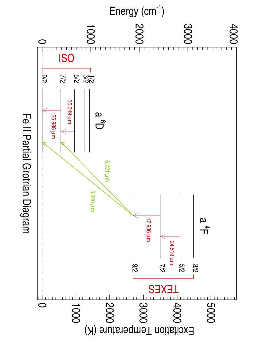
Figure 1: Partial Grotrian diagram showing the forbidden Fe II lines observed with TEXES and ISO.

Figure 1 presents a partial Grotrian diagram of the two lowest energy terms of Fe II showing the characteristic excitation temperature defined as (Energy$/k$). The [Fe II] 25.99 $\mu$m and 35.35 $\mu$m emission lines observed with ISO are from within the ground $4s\>\>a\>^{6}D$ term ($0-977\>{\rm cm}^{-1}$) and probe the cool CSE. Here we use “CSE lines” to refer to emission from within ground energy terms, while the TEXES [Fe II] lines have a hybrid character being from an excited term. For some emission lines this distinction is an oversimplifcation, e.g., for [Fe I] 24.04 $\mu$m where there may be a gradient in the ionization balance (§5.3.1). Observations of the [Fe II] 25.99 $\mu$m and 35.35 $\mu$m kines were obtained with ISO-SWS at spectral resolutions of $R\simeq 1000$ for $\alpha$ Ori, and $R\simeq 250$ for $\alpha$ Sco (Justtanont et al., 1999); these resolving powers are at least a factor of 20 too low to reveal either the turbulence or the flow dynamics. These transitions form a ladder which ends in the ground energy level ($J=9/2$) and can be used to constrain the wind temperature: 35.35 $\mu$m ($J_{ji}=5/2\to 7/2$), and 25.99 $\mu$m ($J_{ji}=7/2\to 9/2$).

An analogous ladder exists within the next term $3d^{7}\>\>a\>^{4}F$ (i.e., the first excited term: $1872-3117\>{\rm cm}^{-1}$): 24.52 $\mu$m ($J_{ji}=5/2\to 7/2$), and 17.94 $\mu$m ($J_{ji}=7/2\to 9/2$). Fig. 1 shows these ladder sequences. These $3d^{7}\>\>a\>^{4}F$ transitions have been observed previously by Kelly & Lacy (1995) in $R\sim 10,000$ Irshell spectra (Lacy et al., 1989) of the $\alpha$ Sco (Antares) system and there is also weak coincident emission in the ISO $\alpha$ Ori spectrum. Since the emission lines present in the ISO spectra are unresolved, the emission line to continuum flux contrast will increase with increasing spectral resolution until the lines become resolved. The TEXES spectral resolution of $R\sim 50,000$ provides an opportunity to detect these lines, resolve their line profiles at the $6\>{\rm km\>s}^{-1}$ level, and, with good signal-to-noise ratio, determine the emission centroid velocities to $\sim 1\>{\rm km\>s}^{-1}$.

The 17.94 $\mu$m line lies in a spectral region with water features, both telluric and photospheric. A narrow telluric water line very close to the [Fe II] line can make the 17.94 $\mu$m feature difficult to interpret, depending on the Doppler shift. In contrast, the 24.52 $\mu$m line lies in a spectral region where the telluric attenuation varies very slowly across the line profile, making it more suitable for detailed emission profile analysis. In Table 1 we give the radiative atomic data for these diagnostics.

There is also potential emission from between the $a\>^{4}F$ and $a\>^{6}D$ terms, namely 6.72 $\mu$m and 5.34 $\mu$m which are also shown in Figure 1. A characteristic of the forbidden transitions in the lowest terms of Fe II is that the radiative rates within a term are stronger than the rates between the terms (Nussbaumer & Storey, 1988). These lines are therefore expected to have weaker emission than the 17.94 $\mu$m and 24.52 $\mu$m lines and also to sit upon a brighter, more complicated, stellar continuum.

2.1 Atomic Data

2.1.1 Radiative Data

To utilize the high spectral resolution of the TEXES data requires accurate wavelengths, or wavenumbers, to establish the Doppler shifts of the line emission. We have adopted the most accurate laboratory wavenumbers of $407.8434\pm 0.0009\>(1\sigma)\>{\rm cm}^{-1}$ (24.52 $\mu$m) and $557.5364\pm 0.0008\>(1\sigma)\>{\rm cm}^{-1}$ (17.94 $\mu$m) which are from an ongoing project at Lund Observatory to improve atomic data for forbidden iron lines (Aldenius & Johansson, 2007). The $1\sigma$ uncertainties correspond to 0.66 and 0.43 ${\rm km\>s}^{-1}$, respectively.

Accurate Einstein decay coefficients ($A_{ji}$) are also required if these lines are to provide thermodynamic constraints. Garstang (1962) calculated the magnetic dipole and electric quadrupole transition probabilities for the 24.52 $\mu$m and 17.94 $\mu$m lines, with the magnetic dipole decay probabilties completely dominating. More recent computations by Nussbaumer & Storey (1988) and the IRON Project SUPERSTRUCTURE code presented by Quinet, Le Dourneuf & Zeippen (1996) are both in good agreement. The latter two sources give $A_{ji}$’s that are the same, which we adopt here, and these in turn are the same as the Garstang (1962) values at the precision of his Table III.

2.1.2 Collisional Data

To establish whether the Fe II energy levels of the emitting plasma are in Local Thermal Equilibrium (LTE) or non-LTE, requires collision rates in and between the Fe II $a\>^{4}F$ and $a\>^{6}D$ terms. Pradhan & Zhang (1993) presented electron collision rate coefficients for forbidden IR Fe II transitions that have an estimated uncertainty of 10-30%. Recently, however, Ramsbottom et al. (2007) presented electron collision rates for temperatures that encompass those expected in M supergiant atmospheres that are lower by a factor of 2. These uncertainties are small in comparison with estimates of hydrogen collision rates.

Detailed collision rates for neutral hydrogen collisions have not been calculated, but estimates have been made for de-excitation rates that are of order $10^{-9}\>{\rm cm}^{3}{\rm s}^{-1}$ (Aannestad, 1973; Bahcall & Wolf, 1968). These are uncertain by an order of magnitude. If hydrogen is partially ionized then the total collision rates will be dominated by electron collisions, but in a cool photoionized stellar wind hydrogen and electron collision rates may be comparable. However, if the gas has a sufficiently high hydrogen density then the Fe II level populations have a Boltzmann (LTE) distribution and the 24.52 $\mu$m and 17.94 $\mu$m diagnostics will then be insensitive to the collision rates and sensitive to the accurately known Einstein A-values. Large mass column densities will also tend to inhibit photon losses and drive the level populations towards LTE.

In §5.2.1 we find that in the line forming region the Fe II $a\>^{4}F$ and $a\>^{6}D$ terms are close to collisional equilibrium so that current uncertainties in theoretical collisional excitation rates are of minor consequence to the interpretation of these mid-IR lines.

3 TEXES OBSERVATIONS

We have observed a sample of M supergiants, given in Table 2, with TEXES in high-resolution mode on the 3 m IRTF on Mauna Kea. The data described here were mostly obtained in 2004 October, 2005 January, and 2005 December (see Table 2 for dates). These observations are the longest wavelengths observed with TEXES, and were facilitated by a CdTe window that replaced the previous KBr window. For the long wavelength observations we used a 2″  slit width (in the dispersion direction) to obtain the maximum spectral resolution and typically nodded 6″  along the 17″  slit to subtract the sky emission. The detector pixels have a linear size of 0.33″, providing a fully sampled Line Spread Function (LSF). The nodded star observations were interleaved with observations of a black thermal source and the sky. For our TEXES observations, very bright astrophysical sources with smooth continua suitable for flat fielding, such as asteroids, were not often available. We therefore used the black thermal source and sky observations to provide an approximate flat field. We derived a first order correction for telluric features, and an estimate of the sky and telescope transmission as described in Lacy et al. (2002). The source flux ($F_{\nu}$), uncorrected for slit losses, is then given by

$$F_{\nu}\simeq S_{\nu}\left({\rm obj}-{\rm sky}\right){B_{\nu}\left(T_{amb}\right)\over{S_{\nu}\left({\rm black}-{\rm sky}\right)}}$$ (1)

where $B_{\nu}\left(T_{amb}\right)$ is the Planck function for the calibration source at temperature, $T_{amb}$, and $S_{\nu}$ is the recorded signal.

The data were collected and initially examined at the telescope using a near real-time reduction package written in the Interactive Data Language (IDL) which facilitated an efficient observing strategy. After the observing run the data were carefully optimized during re-calibration with the pipeline reduction software. The spatial profile on the detector, FWHM $\sim 2.5$″, was used to create a template to extract the stellar spectrum.

We observed the wavelength regions covering the [Fe II] lines discussed in §2, as well as some of the transitions between the $a\>^{4}F$ and $a\>^{6}D$ terms, and also the ground term [Fe I] 24.04 $\mu$m. Here we report on observations obtained so far; not all stars have been observed at all wavelengths. At long wavelengths, in high-resolution mode, only a portion of 4 spectral orders are recorded on the detector at one time. The recorded regions are only about $200\>{\rm km\>s}^{-1}$ wide and do not overlap. Because the features we observe are 20% of the order width, care must be taken to observe spectral features close to the center of the detector. An example of the spectral orders observed for the long wavelength lines in $\alpha$ Ori is shown in Figure 2.

3.1 Wavelength Calibration

The wavelength scale was established by identifying telluric molecular features in adjacent orders. The wavelength calibration of the 24.52 $\mu$m line, however, requires special mention. Finding suitable telluric features near this line proved impossible, so two different wavelength solutions were examined. In the first case, the [Fe II] line was observed in 2nd-order and then the filter was changed to observe a telluric feature in the 12 $\mu$m region in 4th-order. The grating equation was used to establish the 2nd-order wavelength solution. Another solution was established using telluric features about 8-orders from the emission feature. Both methods agree to $1{\rm km\>s}^{-1}$ which is the level of desired accuracy for this science.

3.2 Line Spread Function (LSF)

The LSF was examined prior to mounting TEXES on the telescope using calibration water vapor spectra obtained from a low-pressure gas cell placed on the instrument entrance window. In the high resolution cross-dispersed operating mode with a 2″  slit (in the dispersion direction) the water lines near 24$\mu$m have emission cores that are well characterized by a Gaussian with $R=\lambda/\Delta\lambda_{FWHM}\simeq 51,700\pm 1600$. At $20\mu$m the resolution is $\sim 65,000$. The wings of the LSF are hard to quantify because the water lines sit upon a continuum. In the following analysis we adopt a Gaussian LSF with $R=52,000\>[24/\lambda(\mu{\rm m})]$.

3.3 Gemini-N Observations of $\alpha$ Scorpii (Antares)

During the TEXES Gemini-North engineering run in 2006 February, a spectrum was obtained of the [Fe II] 24.52 $\mu$m line in Antares on Feb 24. Unfortunately, no absolute wavelength calibration was obtained. The slit was oriented north-south, perpendicular to the direction to the B 2.5 V star companion. The slit was roughly 6″ long and we nodded the telescope east by 4″ to remove sky emission and avoid potential contributions from the companion that lies 3″ west. The spectral resolution determined by the gas cell prior to the observing run was R=60,000 at 18.8 $\mu$m, which suggests, via the scaling law used above, a spectral resolution at 24 $\mu$m of $6.4\>{\rm km\>s}^{-1}$.

These data were reduced in the same manner as the IRTF data.

4 RESULTS

4.1 Detections

The stellar continuum near 17.94 $\mu$m is quite structured in these evolved, oxygen-rich M stars, and current limitations of theoretical M supergiant photospheric spectra preclude us from making positive detections unless the emission line stands above the adjacent continuum. In addition, the telluric interference near the 17.94 $\mu$m line, depending on its Doppler shift, can make this line difficult to analyze. We observed additional evolved K and M stars with widely different surface gravities and mass-loss rates to provide an empirical check on the structure of stellar photospheric continua. A summary of the observations and line detections is given in Table 2. At 24.5 $\mu$m the continuum is less structured but TEXES is not as sensitive. However, the 24.5 $\mu$m setting proved useful in establishing the presence of [Fe II] emission. We have dectected [Fe II] emission from all six of the M supergiants that we have observed.

Figure 2 shows our first observations of $\alpha$ Ori at all three wavelength settings. As mentioned before, we record only a portion of four orders at these wavelengths. The figure shows how the 17.94 $\mu$m line might be affected by a telluric water feature, while the sky transmission is smooth for the other two lines. The [Fe II] lines are much stronger than the ground term [Fe I] line which, when the emissivities are considered, shows that iron is predominantly singly ionized in the extended atmosphere.

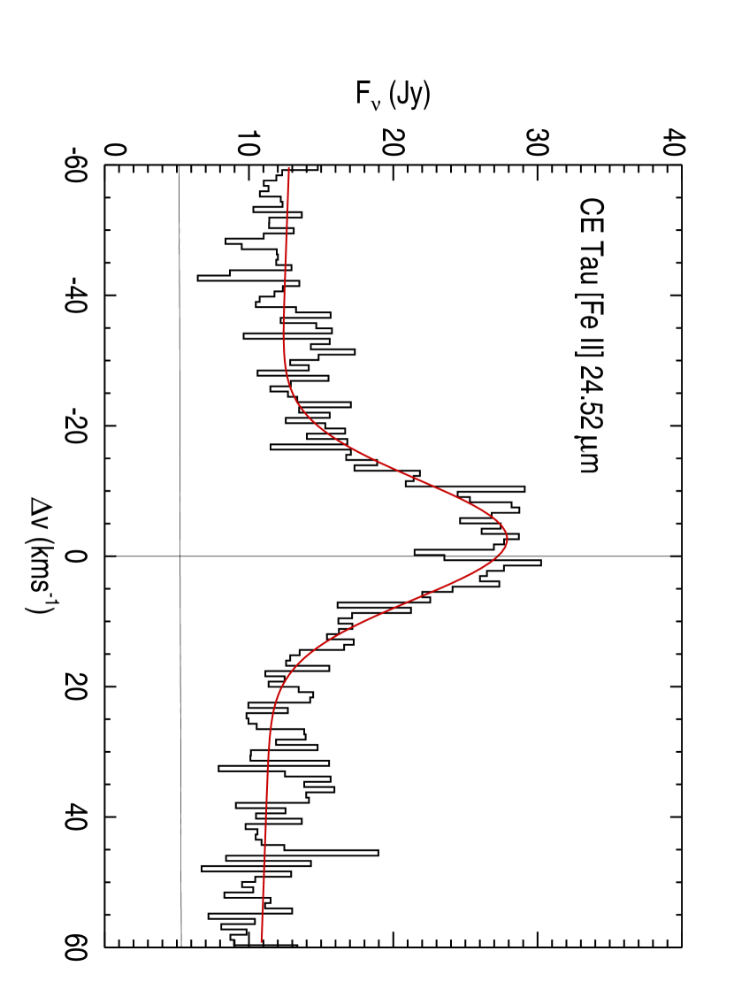
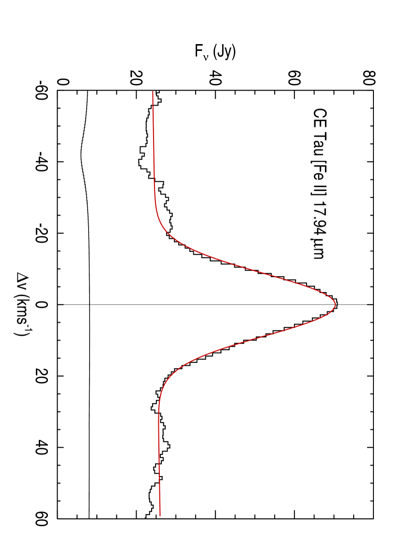
Figure 3: [Fe II] 17.94 $\mu$m and 24.52 $\mu$m emission lines in CE Tau (M2 Iab). The abscissa is the Doppler velocity in the stellar rest frame, and the ordinate is the flux which has been flat-fielded, but not put onto an absolute scale. The shape of the sky transmission is shown beneath the spectrum. CE Tau is a spectral-type proxy for $\alpha$ Ori and the line centroid and widths for these two stars are very similar. This star has weak (or absent) dust emission.

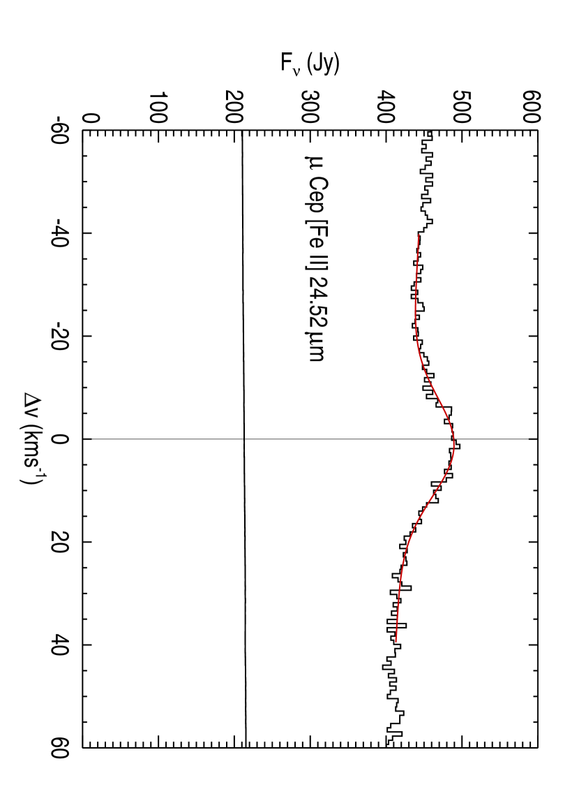
Figure 4: [Fe II] 17.94 $\mu$m and 24.52 $\mu$m emission lines in $\mu$ Cep (M2 Ia). The axes are the same as described in Fig. 3. This supergiant has stronger silicate dust emission that $\alpha$ Ori which is a contributing factor to the low emission line to continuum ratio.

A comparison of $\alpha$ Ori with CE Tau (M2 Iab) and $\mu$ Cep (M2 Ia) illustrates the effect of emission from circumstellar oxygen-rich dust (Sloan & Price, 1998) on the line-to-continuum ratio. Figure 3 shows the the Fe II emission for CE Tau which is a close spectral-type proxy for $\alpha$ Ori and the line profiles are very similar. The line to continuum ratio is, however, substantially larger than observed in $\alpha$ Ori and this is, at least in part, a result of the much weaker (or absent) dust emission from CE Tau. $\mu$ Cep (shown in Figure 4) has much stronger silicate dust emission and a greatly reduced line to continuum contrast. In $\mu$ Cep the 17.94 $\mu$m line is also detected but the two lines appear to have differently shaped profiles and the less symmetric 17.94 $\mu$m line is slightly redshifted with respect to the adopted $V_{rad}=+19.4\>{\rm km\>s}^{-1}$. This may be a result of underlying photospheric molecular features.

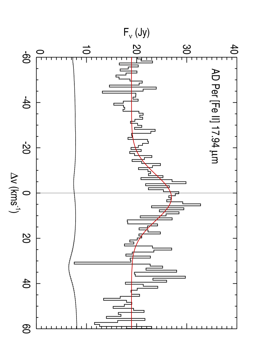
Figure 5: [Fe II] 17.94 $\mu$m emission line in AD Per. The axes are the same as described in Fig. 3. This is the most distant M supergiant in the sample at $\sim 2$ kpc and has a mass-loss rate similar to nearby $\alpha$ Ori and $\alpha$ Sco which are $\sim 200$ pc.

We also observed AD Per (M2.5 Iab), our most distant source at $\sim 2$ kpc, and detected the 17.94 $\mu$m line which is shown in Figure 5. This star appears to have unusual dust chemistry with carbon-rich dust (SiC) but an oxygen-rich photosphere (Skinner & Whitmore 1988; Skinner et al. 1990).

The difference between $\alpha^{1}$ Her (M5 II) and $\beta$ Peg (M2.5 II-III) in the 17.9 $\mu$m region is shown in Figure 6 which reveals a narrow emission component near the stellar rest frame of $\alpha^{1}$ Her. Subsequent 24.52 $\mu$m observations, not described here, confirm the [Fe II] emission. Both $\alpha$ Her’s [Fe II] profiles are slightly narrower than in the more luminous counterparts. This figure illustrates the difficulty of identifying the emission line in this wavelength region, in the absence of reliable synthetic stellar spectra, when the emission is comparable in strength to the continuum.

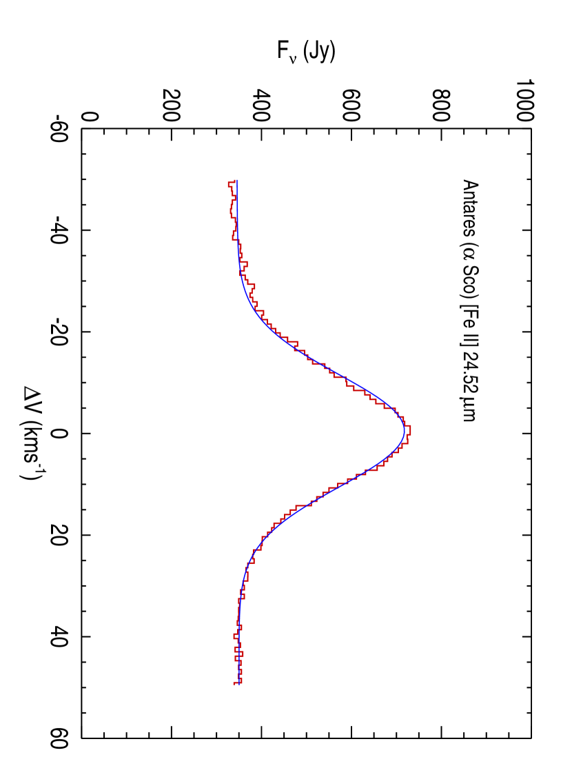
Figure 7: [Fe II] 24.52 $\mu$m emission line in Antares. This spectrum was obtained with Gemini-N during an engineering run on 2006 February 24. The axes are as described in Fig. 3. The smooth profile is a Gaussian fit to the emission feature. No absolute wavelength scale was obtained for this spectrum.

The 24.52 $\mu$m line of $\alpha$ Sco shown in Figure 7 is slightly wider than for the other stars (see Table 3), however we find no indication of extended emission. The Antares nebulae is a source of rich optical Fe II emission, e.g., Swings & Preston (1978), which is excited by the nearby B star companion (separation of 2.7″) (Reimers et al., 2008). TEXES observations of this system may be sampling material from a slightly more extended, but still spatially unresolved, region than for the single stars, and this material may have different velocity fields.

4.2 Properties of Line Profiles

To characterize the observed emission, Gaussian profiles have been fit to the spectra and their properties are given in Table 3. $\alpha$ Ori was observed on several occasions and we have also flux calibrated these spectra as described in Appendix A. The fits to these individual spectra are given in Table 4 which provides an indication of the reproducibility of the spectra and of the intrinsic variability.

The centroid emission velocities are given with respect to the adopted stellar (center-of-mass) radial velocities which have typical uncertainties of at least $1\>{\rm km\>s}^{-1}$. For M supergiants the center-of-mass radial velocities are not very well determined because there are photospheric radial velocity variations, e.g., Jones (1928), typically with amplitudes of $\pm 3-5\>{\rm km\>s}^{-1}$, that have both semi-regular (often with multiple periods of hundreds of days to several years) and short-term erratic variations, e.g., Smith et al. (1989). So at any given time the photosphere has a strong likelihood of moving with respect to the center-of-mass. Few M supergiants have been monitored for sufficient lengths of time to determine $V_{rad}$ with sub-${\rm km\>s}^{-1}$ accuracy.

The observed emission centroid velocities are all close to the stellar center-of-mass radial velocities which suggests that the [Fe II] emission is not formed in the convective churning photospheres which undergo velocity fluctuations seen in optical absorption features. It is more likely that the emitting region is larger and, or, decoupled from the variable surface layers. For $\alpha$ Ori we observe little, if any, variation with time which further supports this conclusion. During the 14 month period of our observations $\alpha$ Ori’s photospheric apparent velocity spanned a range of at least $3.7\>{\rm km\>s}^{-1}$ (Gray, 2008), although we do not have enough epochs in common to study possible correlations. It is well known that the chromosphere and wind of $\alpha$ Ori is decoupled from its photospheric variations (Goldberg, 1979). What is apparent is that the [Fe II] emission profiles are neither blue-shifted nor are they flat-topped. Both of these properties exclude the possibility that the emission is formed with any significant outflow velocity, typically $\sim 10\>{\rm km\>s}^{-1}$ for M supergiants. If the emission were from within such a moving flow, the absence of blue shifted profiles excludes the flux being formed close to the star, while the absence of a top-hat profile excludes the emission originating from an extended region. We conclude the emission arises from material with at most a small outflow velocity. Further consideration of the line formation in §5.1 reveals that the emission arises from close to the star.

The observed line profiles are well resolved. Because the cores of the TEXES LSF and observed profiles are quite Gaussian, the intrinsic stellar most probable turbulent velocity ($V_{turb}$), which we assume to be isotropic , can be estimated from

$$V_{turb}=\sqrt{V_{Dopp}^{2}{\rm(Obs)}-(X\>{\rm km\>s}^{-1})^{2}},$$ (2)

where $X=2.6$ and $3.5\>{\rm km\>s}^{-1}$ are the corrections for the TEXES instrumental broadening at 17.94 and 24.52 $\mu$m, respectively. The observed [Fe II] line widths given in Tables 3 and 4 are similar with a range of $V_{turb}=12-15\>{\rm km\>s}^{-1}$ with $\alpha$ Sco having the largest value.

For $\alpha$ Ori, the [Fe II] line widths are similar for both the 17.94 $\mu$m and 24.52 $\mu$m lines ($\simeq 12.5$ $\>\mathrm{km\>s}^{-1}\>$) and they do not change significantly between the three different observing runs. The 24.04 $\mu$m [Fe I] line is significantly narrower and indicates a different line forming region. Both of these forbidden line widths are significantly less than that derived from the chromospheric UV C II] 2325 Å emission multiplet. The sky integrated C II] profiles observed with HST have non-Gaussian profiles whose FWHM implies $V_{turb}=19-21$ $\>\mathrm{km\>s}^{-1}\>$(Carpenter & Robinson, 1997). Radiative transfer modeling of the spatially resolved HST/STIS C II] 2325 Å emission reveals that these lines are slightly opacity broadened at the stellar limb and can be well matched with intrinsic turbulence of $V_{turb}=17-19$ $\>\mathrm{km\>s}^{-1}\>$which changes slowly over large spatial scales: $1.5R_{\ast}<R<3.5R_{\ast}$ (Harper & Brown, 2006). This is the same spatial region over which we anticipate that the [Fe II] emission originates.

The cool component of $\alpha$ Ori’s inhomogeneous atmosphere, traced by thermal radio continuum observations, has now been dynamically resolved from the hot component, traced by UV emission lines, for the first time. The [Fe II] profiles, with their much lower temperature sensitivity, reflect the amplitude of the motions in the cooler plasma which are less than that of the hotter chromosphere. Since the cool atmospheric component includes the base of the wind outflow, it is these lower amplitude motions that should be associated with the unknown wind driving processes. For 1000-3500 K plasma these turbulent velocities, if interpreted as occurring on small spatial scales, imply significant Mach numbers. While the TEXES [Fe II] profiles are spatially unresolved (they are global averages), there is no evidence for outward travelling shocks moving with these velocities in the line forming region.

For our TEXES [Fe II] detections the turbulent velocities are similar in all stars, which may not be a surprise since the sample consists of mostly early M supergiants. The remarkable discovery by Lim et al. (1998) that the extended atmosphere of $\alpha$ Ori is dominated by cool, rather than hot gas as previously thought, has now been confirmed for $\alpha$ Sco with VLA A-configuration observations made by Brown & Harper (Harper, 2009). The presence of extended cool non-chromospheric plasma with $V_{turb}\simeq 13$ $\>\mathrm{km\>s}^{-1}\>$is likely a common property of early M supergiants and not a rare curiosity, and deserves further attention.

These [Fe II] turbulent velocities are larger than the macroturbulence required to model upper photospheric 12 $\mu$m molecular OH and H₂O absorption lines of $\mu$ Cep (Ryde et al., 2006b) and $\alpha$ Ori (Ryde et al., 2006a). The 8 $\>\mathrm{km\>s}^{-1}\>$turbulence required to match $\alpha$ Ori’s 12 $\mu$m TEXES spectrum in Ryde et al. (2006a) is actually smaller than that needed to model the optical: 11 $\>\mathrm{km\>s}^{-1}\>$(Gray 2000, 2008) and $\sim 15$ $\>\mathrm{km\>s}^{-1}\>$Gray 2001), and near-IR: 12 $\>\mathrm{km\>s}^{-1}\>$(Lobel & Dupree, 2000) photospheric lines. The conclusion to be drawn from this is that as absorption lines are formed farther out from the star, they become less sensitive to the vigorous photospheric convective motions, which in turn is reflected in the lower macroturbulence required to match the observed line widths. At some radius where the extended atmosphere becomes decoupled from the photosphere, the turbulent motions increase once more in both the hot chromospheric and cool wind components.

4.3 Thermal Constraints

To place the dynamical information from the resolved line profiles in better context we need to establish where the emission is formed. In this subsection we will consider the most general formation properties and then in §5 we will consider the contribution functions of the TEXES and ISO CSE lines from $\alpha$ Ori in more detail.

The characteristic formation temperature can be derived by assuming that the relative level populations of the upper (j) and lower (i) energy levels $(n_{j},n_{i})$ can be described by a Boltzmann distribution with a characteristic excitation temperature $(T_{exc})$ where

$${n_{j}\over{n_{i}}}={g_{j}\over{g_{i}}}\exp\left\{-(E_{j}-E_{i})/kT_{exc}\right\}.$$ (3)

The $g$’s are the statistical weights, and $E_{j}-E_{i}$ is the energy difference between the upper and lower energy levels. If the wind is isothermal and the energy levels are in thermal equilibrium then $T_{exc}=T_{gas}$. From the Einstein A-values and by assuming optically thin emission for the ratio of the ISO fluxes, Justtanont et al. (1999) derive excitation temperatures for the ground term emission of $T_{exc}\simeq 1785$ K and $T_{exc}\simeq 1230$ K for $\alpha$ Sco and $\alpha$ Ori, respectively. From the ratio of populations in the ground $a\>^{6}D$ and excited $a\>^{4}F$ terms the TEXES $\alpha$ Ori Fe II fluxes give $T_{exc}\sim 1520-1950$ K. Since in $\alpha$ Ori the ground state emits at a lower characteristic temperature, this provides a lower limit for $T_{exc}$ for the $a\>^{4}F$ excitation region. For the ratio of fluxes within the $a\>^{4}F$ term we find a $3\sigma$ lower limit of $2110$ K, so the atmosphere is not isothermal.

Figure 10 (in Appendix B) shows the composite temperature structure for $\alpha$ Ori described in Appendix B and also shows the formation radii based on the ISO and TEXES temperature constraints under these simple isothermal and optically thin assumptions. In the theoretical model of Rodgers & Glassgold (1991) the $a\>^{6}D$ ground term emission originates near $\sim 10R_{\ast}$, however, we now know from the thermal radio continuum observations of Lim et al. (1998) that this temperature must occur slightly closer to the star, i.e., at $\sim 7.4R_{\ast}$. The $a\>^{4}F$ emission originates interior to this at $\leq 4.1R_{\ast}$ where the outflow velocities are expected to be small. This spatial constraint provides a partial explanation of why Doppler blue-shifted wind signatures are not observed.

In summary, we find that the M supergiants share common properties in that their mid-IR [Fe II] line profiles appear to be quite Gaussian (rather than top-hat) and show no evidence of significant Doppler shifts indicative of outflow. To within the combined uncertainties the lines are at rest in the stellar rest frame. The line-to-continuum contrast is a function of the circumstellar dust emission as expected. The characteristic excitation temperature places the line formation close to the star where the outflow velocities are expected to be low, which explains the lack of a clear wind signature. For the case of $\alpha$ Ori the line profiles do not show significant variability and the line widths are systematically smaller than those observed in spatially resolved UV spectra of the hotter chromosphere. We have dynamically resolved the turbulent motions in the dominant and pervasive cool atmospheric component.

5 DISCUSSION: $\alpha$ Orionis in Context

Where are the mid- and far-IR emission lines observed in $\alpha$ Ori with TEXES, KAO, and ISO formed? To quantify the emission contributions from different radii, a thermodynamic and dynamic model is required that encompasses the chromosphere, inner wind, and CSE. Currently no such comprehensive models exist. $\alpha$ Orionis provides the best studied example of an M supergiant and we will use the properties of this star throughout this section to quantify the mid- and far-IR line emission, with the reasonable assumption that the results will apply at some level to early M supergiants in general.

While no complete atmospheric model exists, models do exist for the inner region (Harper et al., 2001, HBL01 hereafter) and the outer CSE (Rodgers & Glassgold, 1991, RG91 hereafter). Appendix B describes a spherical (1-D) composite dynamic ($V_{turb}(R)$, $V_{wind}(R)$) and thermodynamic ($T_{gas}(R)$, $\rho(R)$) model that utilized these earlier results and interpolates between them. This composite model is essentially a combination of the spatially extended semi-empirical model of HBL01 scaled to the recently revised stellar distance (Harper et al., 2008) and one of the variational thermodynamic models of RG91, and is referred to as the Composite Model Atmosphere. In the following calculations we use the cooler inner wind model which is shown as a dashed line in Fig. 10 in Appendix B.

The HBL01 inner region model was based upon multiwavelength spatially-resolved VLA data covering 0.7-6 cm combined with non-contemporaneous spatially unresolved data at shorter wavelengths. The HBL01 model predicts a thermal continuum flux at 100 GHz (0.3 cm) of 92.2 mJy which is insensitive to the wind dust emission. As part of a larger multiwavelength study of M supergiants and to provide a check on temporal changes in the extended atmosphere of $\alpha$ Ori, we obtained observations of $\alpha$ Ori, $\alpha$ Sco and $\alpha$ Her at 100 GHz with the OVRO Millimeter Array and these are described next.

5.0.1 Owens Valley Radio Observatory (OVRO)

The OVRO observations of $\alpha$ Ori, $\alpha$ Sco, and $\alpha$ Her are summarized in Table 6. For $\alpha$ Ori, observed on 2003 November 9, four 1 GHz continuum bands were observed with the dual-channel analog correlator centered around 100 GHz and spanning the range 96.5-103.5 GHz. The antennae were in the L configuration with baselines between 15-115 m, although only 5 antennas were available during the observation. The instrumental gain was calibrated every 15 minutes using the quasar J0532+075. The absolute flux was bootstrapped from J0923+392 observations, because no planets were available during the $\alpha$ Ori transits, resulting in a 15% uncertainty in the absolute flux scale. The calibrations were done with the OVRO MMA software (Scoville et al., 1993) and the images were produced using standard routines in Miriad (Sault, Teuben, & Wright, 1995).

For $\alpha$ Sco and $\alpha$ Her, observed in a shared track on 2004 March 30, the gains were calibrated using the quasars J1517-243 and J1608+104, respectively and fluxes were bootstrapped from these two quasars with a similar 15% uncertainty. The correlator setup was the same as for $\alpha$ Ori. This track was taken in E configuration which contains several more extended baselines than L with baselines between 35 and 119 m and all 6 antennae were present throughout the track.

It is interesting to compare the 100 GHz fluxes with the 250 GHz fluxes measured by Altenhoff et al. (1994) and shown in Table 6. At these high frequencies the earlier spectral-type companions of $\alpha$ Sco and $\alpha$ Her should have negligible flux contributions, e.g. Hjellming & Newell (1983). The 250/100 GHz flux ratios for $\alpha$ Sco, $\alpha$ Ori, and $\alpha$ Her are $4.9\pm 0.5$, $4.4\pm 0.4$, and $5.5\pm 0.5$, respectively. When the 100 GHz fluxes are normalized to the product of the star’s effective temperature and angular diameter squared, e.g., from Dyck et al. (1996), the two luminosity class Iab M supergiants ($\alpha$ Ori and $\alpha$ Sco) have similar ratios (within 10%) while for the less luminous $\alpha$ Her, the ratio is about half this value, which may reflect it’s less massive extended atmosphere.

The HBL01 model predicted a 100 GHz flux (92 mJy) which is consistent with the rather uncertain 90 GHz fluxes recorded in 1975 (Newell & Hjellming 1982 and references therein). Our OVRO $\alpha$ Ori flux was recorded about a year before the first TEXES observations and is slightly lower which may reflect the mean atmospheric temperature being slightly cooler than adopted in HBL01.

5.1 Line Formation

Here we examine the line formation of the forbidden excited [Fe II] and ground term CSE lines by computing their emission profiles and contribution functions. We assume that the source functions of the relevant forbidden lines are in Local Thermal Equilibrium (LTE), i.e., $S_{\nu}\simeq B_{\nu}\left(T\right)$. This can be a reasonable approximation when the particle densities in the line formation region are greater than the critical densities. These conditions can be checked a posteriori and are discussed further in §5.2.1.

We include the wind and turbulent velocity fields in the atomic absorption profile (which is assumed equal to the emission profile, i.e., complete redistribution) and compute the resulting spectral profiles from the formal solution of the equation of radiative transfer in a spherical atmosphere which runs from the upper photosphere through to the CSE.

The adopted abundances and Einstein decay coefficients are given in Tables 1 and 7. For the thermal conditions in the extended envelope, stimulated emission is important for these mid- and far-IR transitions. The background continuous opacity is dominated by pure absorption and has contributions from bound-free opacity from excited levels of neutral species, and H and H^- free-free opacity. At these wavelengths, the bound-free opacity comes from hydrogenic quantum numbers $n\geq 14$, which are likely to be partially collisionally coupled to the continuum, so that both bound-free and H free-free opacity are proportional to the electron density. We performed trial non-LTE calculations for the populations of the hydrogenic Rydberg $(n,l)$ states, following Hummer & Storey (1992), and found that, at the large column densities where the continuum opacity is important for these mid- far-IR lines, the departure coefficients of the $(n,l)$ levels are not significantly different from unity. The continuous opacity is important in the deeper layers because of the density sensitivity, $\kappa_{cont}\propto n_{e}n_{H}$, and the continuum sets the inner boundary condition for the line formation problem. The modelled line fluxes were obtained by measuring the emission above the computed local continuum and are given in Tables 5 and 8.

5.2 Flux Contribution Functions

An alternate way to estimate the line fluxes is to sum up the emission from each volume element in the extended atmosphere and wind, i.e.,

$$F_{\oplus}\simeq{h\nu_{ji}A_{ji}\over{D^{2}}}\int\limits_{R_{\ast}}^{\infty}n_{H}{n_{FeII}\over{n_{H}}}{n_{j}\over{n_{FeII}}}P_{esc}(R)R^{2}\>dR={h\nu_{ji}A_{ji}\over{D^{2}}}\int\limits_{R_{\ast}}^{\infty}n_{H}{n_{FeII}\over{n_{H}}}{n_{j}\over{n_{FeII}}}P_{esc}(R)R^{3}\>d\ln{R}$$ (4)

where $D$ is the distance to the star, $h\nu_{ji}$ is the photon energy, $A_{ji}$ is the Einstein decay coefficient, $n_{H}$ is the total hydrogen population, $n_{FeII}/n_{H}$ is the abundance of Fe II relative to hydrogen ($=A_{FeII}$), $n_{j}/n_{FeII}$ is the ratio of the population of the upper emitting level to the total Fe II population, and $P_{esc}(R)$ is the single-flight escape probability of the photon emitted at radius $R$. This escape probability is adopted because the particle densities are high enough that the probability of a photon scattering and subsequently escaping is small. The high particle densities indicate that fine-structure level populations will be close to a Boltzmann distribution, so that

$${n_{j}\over{n_{FeII}}}\simeq{g_{j}\over{U(T_{gas})}}\exp\left\{-E_{j}/kT_{gas}\right\}$$

where $U(T_{gas})$ is the non-LTE partition function of Fe II, and $E_{j}$ is the energy of the emitting (upper) level with respect to the ground energy level.

The inner boundary is chosen to be deep enough that $P_{esc}\left(R\right)\to 0$. The escape probability takes into account photons that are thermalized during line scattering and by continuum absorption. For low optical depths at a few stellar radii $P_{esc}$ is approximately the fraction of the sky not subtended by the star and rapidly approaches unity as the radius increases. Closer to the star $P_{esc}$ allows for photons that escape in the wings of the emission line when the line center optical depth is greater than unity.

To illustrate where the emission lines originate we define a radially weighted contribution function

$$C_{rw}=n_{H}{n_{FeII}\over{n_{H}}}{n_{j}\over{n_{FeII}}}P_{esc}(R)R^{3}$$ (5)

such that, when plotted against $\ln{R}$, the area under the curve shows the relative contribution of different regions to the total flux. While the formal solution of the transfer equation provides, in principle, an exact $P_{esc}(R)$, here we use Eq. (5) to illustrate $C_{rw}$.

Convenient expressions for the escape probability have been derived for plane parallel geometry and certain spherical distributions of static scattering material (Kunasz & Hummer, 1974). For stellar winds where $V_{wind}>V_{turb}$ the Sobolev escape probability is often employed (Castor, 1970). Normalizing radial distances by the stellar radius, i.e., $Z=R/R_{\ast}$, the continuum radial optical depth of unity occurs close to the stellar surface at $Z_{cont}$. Here we approximate $P_{esc}(R)$ as the larger of the Sobolev value or

$$P_{esc}\left(R\right)=K_{2}\left(\tau\right)E_{2}\left(\tau_{cont}\right){1\over{2}}\left[1+\sqrt{1-\left({Z_{cont}\over{Z}}\right)^{2}}\right]$$ (6)

where $K_{2}$ is the half-sky plane-parallel Doppler profile single-flight escape probability given by Hummer (1981) with the mean optical depth of a static atmosphere. The $E_{2}$ term approximates the fraction of line photons not lost to the continuum and is only important close to the star. The geometric term allows for stellar occultation, and the factor $Z_{cont}\sim 1.2$ is the radius where the tangential continuum optical depth is unity.

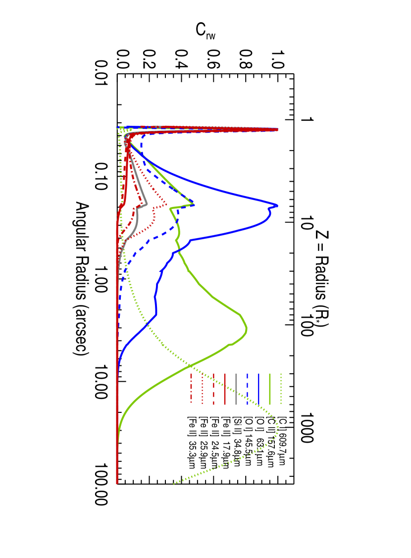
Figure 8: Contribution functions for the emission lines observed in $\alpha$ Ori with TEXES, ISO and the KAO. The area under each curve gives the relative flux contribution. The narrow peak at $Z\sim 1.45$ is the contribution from the relatively dense inhomogeneous region that includes the hot chromosphere.

Figure 8 shows the normalized $C_{rw}$ for the TEXES and CSE lines. The narrow peak at $Z\simeq 1.5$ corresponds to the high particle densities and maximum temperatures in the Composite Model with the sharp cut-off on the photospheric side resulting from continuum absorption which affects all lines in a similar fashion and eliminates any photospheric contributions to the emission fluxes. The decline outward of the peak is a combined result of the declining $T_{gas}$ and density. Previous generations of theoretical, e.g., Hartmann & Avrett (1984), and semi-empirical models, e.g., Wischnewski & Wendker (1981) and Lobel & Dupree (2000), had more extended warm chromospheres. Most of these can be ruled out by the observed narrowness, the absence of observed blue-shifts or wind broadening in the TEXES [Fe II] profiles. The small discontinuity in the figure at $Z\simeq 7$ reflects where the density structure of the outer wind has been merged with the inner density structure that is constrained by radio observations (see Appendix B).

The TEXES and ISO [Fe II] lines clearly have different formation radii as previously suggested by their different characteristic excitation temperatures. The TEXES lines have half their emission from a region around the peak-$T_{gas}$ ($Z=1.5$) while the ISO lines are formed around $Z\sim 6$. The absence of wind shifted emission in the TEXES lines is a result of the significant contribution from the quasi-static region at chromospheric radii and above. It is thought that this extended region, resolved with the VLA by Lim et al. (1998), is in the base of the wind where the velocity is small (Harper et al., 2001) and thus the TEXES [Fe II] lines are probing the wind, albeit at low outflow velocities.

Fig. 8 suggests that the wind acceleration signature might be apparent in the ground term [Si II] 34.81 $\mu$m and [Fe II] 35.34 and 25.98 $\mu$m profiles if observed with sufficient spectral resolution. Note that these lines have a non-negligible flux contribution from within $3R_{\ast}$ which, however, is often taken as the inner boundary condition (Rodgers & Glassgold 1991; Haas & Glassgold 1993; Haas et al. 1995; Justtanont et al. 1999). Clearly consideration of the material at $R<3R_{\ast}$ is required for detailed analysis of these mid- far-IR lines.

The [O I], [C I], and [C II] lines are expected to have top-hat profiles and be centered close to the stellar rest frame, as the fraction of red-shifted emission occulted by the star is tiny. Indeed observation of [C I] 609 $\mu$m by Huggins et al. (1994) reveal that this line has similarities to mm-CO emission profiles and suggests that its very broad spatial contribution function also includes material traveling with the faster S2 shell (see Appendix §B2.1).

The [Fe II] emission sits upon upper photospheric/lower chromospheric absorption and more reliable model fluxes require a more detailed description of the $T_{gas}$ structure between the chromospheric $T_{gas}$-rise and the photosphere than available at present. Recent VLTI MIDI 7.5-13.5 $\mu$m observations (Perrin et al., 2007) suggest the presence of a cool molecular rich region with $T_{gas}\sim 1550$ K interior to 1.25$R_{\ast}$ (corrected to the angular diameter adopted here). The presence of molecular material between the upper-photosphere and the chromospheric temperature peak is reminiscent of the bifurcated outer atmosphere observed off the solar limb in CO (Ayres, 2002) albeit on a larger fractional radial scale as befits the lower surface gravity of Betelgeuse. This molecular material may also be related to the detection of water vapor in the outer photosphere of Arcturus by Ryde et al. (2002). Future Atacama Large Millimeter Array (ALMA) interferometric sub-mm continuum observations will provide independent thermodynamic constraints down from the chromosphere towards the photosphere and covering this intriguing molecular region. Such ALMA data will complement those from the VLA that sample the chromosphere and wind.

5.2.1 Line Source Functions

Departures from the assumed LTE line source functions can lead to uncertainties in the contribution functions and line fluxes. Potential departures can be considered by examining the equivalent two-level atom description of the line source function $S_{L}$ (Mihalas, 1978)

$$S_{L}={\bar{J}+\left(\epsilon^{\prime}+\theta\right)B_{\nu}\left(T_{gas}\right)\over{1+\epsilon^{\prime}+\eta}}$$ (7)

where

$$\epsilon^{\prime}\equiv C_{ji}\left(1-e^{-h\nu/kT}\right)/A_{ji}$$ (8)

and $C_{ji}$ is the collisional de-excitation rate. $B_{\nu}(T_{gas})$ is the Planck function at the line frequency, $\bar{J}$ is the mean intensity averaged over the line profile, and the other terms $\theta$ and $\eta$ represent the radiative and collisional coupling between the levels $i,j$ and all other energy levels of the ion, i.e., many possible interactions (see Mihalas 1978 for details).

If the net rate of radiative and collisional coupling between the upper (j) [and lower (i)] level of the mid- and far-IR transition to all other levels, excluding i (or j), can be neglected, (i.e., $\theta\ll\epsilon^{\prime}$ and $\eta\ll\epsilon^{\prime}$) then Eq. (7) reduces to the standard two-level atom description. Under these circumstances, if the downward collision rate for $j\to i$ is higher than the radiative decay rate ($A_{ji}$), then $\epsilon^{\prime}\gg 1$ and the levels are in an LTE ratio with $S_{L}\simeq B(T_{gas})$. Estimates of the critical particle densities required to establish thermal equilibrium between the energy levels of forbidden lines are given in the compilation of Hollenbach & McKee (1989). Although the hydrogen collision rates are very uncertain, typically thermalization requires $n_{H}>10^{4}\>{\rm cm}^{-3}$, which is satisfied for radii $<100R_{\ast}$. This is a necessary, but not sufficient, condition for $S_{L}\simeq B(T_{gas})$ because the coupling between other energy levels embodied by $\theta$ and $\eta$ can be important.

For Fe II, collisions play a particularly important role because the first 64 fine-structure energy levels have the same parity and hence are coupled by collisions that compete with parity conserving electric quadrapole (E2) and magnetic dipole (M1) transitions. Because there are so many energy levels the terms $\theta$ and $\eta$ are not simply evaluated, so to check the accuracy of the LTE source function approximation for the TEXES [Fe II] lines we have examined their source functions. Escape probabilities were used to approximate the net radiative brackets in an Fe II model with the first 769 energy levels for the HBL01 model of $\alpha$ Ori. The atomic data are essentially those described by Sigut & Pradhan (1998). The ratio $S_{L}/B(T_{gas})\simeq 1$ for $R<7R_{\ast}$ with departures of at least 10% occuring in the outer line forming region

Photoexcitation by chromospheric ultraviolet radiation in the allowed transition Fe II multiplets whose lower term is also $a\>^{4}F$, e.g., Multiplet Nos. 20-31 $(A_{ji}\sim 10^{5}-10^{7}\>{\rm s}^{-1})$ (Fuhr & Wiese, 2006) can lead to excitation depopulation rates in excess of the [Fe II] decay rates. These transitions are opaque and the depopulation rates depend on self-shielding which is sensitive to the wind velocity and turbulent gradients. Evaluating these rate is beyond the scope of the present work but we note that detailed non-LTE source functions are desirable for future analysis.

5.3 Observed and Predicted Mid- and Far-IR Fluxes

A comparison of the computed and observed fluxes for $\alpha$ Ori in Tables 5 & 8 reveals a rather unusual mismatch that is a function of formation radius. The computed TEXES [Fe II] fluxes are $\sim 3.1$ too large, the [Si II] and ISO [Fe II] emission lines are $\sim 1.6$ too large, while the lines formed at larger radii are in reasonable agreement with, or slightly underestimate, the more uncertain observations.

There are different uncertainties in the calibrations and flux measurements of these lines (observed with TEXES, ISO, and KAO) that arise from different elements with their inherent uncertainties in abundance and ionization state. However, because of the overlapping formation radii this systematic trend is hard to explain in a simple way. These mid- and far-IR lines have large contributions inside the silicate dust shell observed at $\sim 30R_{\ast}$ (Danchi et al., 1994) and molecular abundances and the dust/gas mass ratio are lower than for cooler M supergiants, suggesting that the CSE flux discrepancy is not a result of depletion from dust formation or molecular chemistry. The combined uncertainties resulting from the observed fluxes and intrinsic variability should be $<30$%, so next we explore other possible explanations.

5.3.1 Ionization Balance?

Iron

The [Fe I] 24.04 $\mu$m emission arises from the ground term and, for a fixed ionization balance, it might be expected to be formed in the same region as the ISO [Fe II] 25.99 $\mu$m line. The observed ratio of TEXES [Fe II] to [Fe I] fluxes in $\alpha$ Ori shows that iron is predominantly singly ionized, in agreement with theoretical calculations of Rodgers (1990). This allows the fluxes of the [Fe II] lines to be used as diagnostics of the amount of material in the extended atmosphere. The [Fe I] 24.04 $\mu$m flux can be reproduced with the Composite Model Atmosphere by assuming a constant $A_{FeI}=10^{-2}A_{FeII}$. However, the narrowness of the profile suggests that it has a stronger contribution from closer to the star where the turbulence is smaller and thus the ionization of iron increases with radius above the surface. The ionization balance in the chromosphere and inner wind region is controlled by the competing forces of photoionization by the strong stellar UV radiation field and radiative recombination. The [Fe I] 24.04 $\mu$m profile is less Gaussian and slightly asymmetric as compared to the TEXES [Fe II] lines and possibly has a small blue shift, in which case the [Fe I] may have a wind emission component.

Castro-Carrizo et al. (2001) have reported a [Fe I] 24.04 $\mu$m flux from ISO grating spectra of $3.5\pm 0.4\times 10^{-19}\>{\rm W\>cm}^{-2}$ which is significantly larger than we estimate from our TEXES spectra ($7.7\pm\times 10^{-20}\>{\rm W\>cm}^{-2}$) which has a factor 40 greater spectral resolution. Fig. 2 reveals that there is another emission feature nearby which would be unresolved in ISO spectra might account, in part, for the difference in measured flux. We are unable to identify this feature, but it is redshifted roughly 28 $\>\mathrm{km\>s}^{-1}\>$from the peak of the [Fe I] emission. Therefore, we believe it is unlikely to be a separate component of [Fe I]. Aoki et al. (1998) have also reported the detection of this [Fe I] line in ISO spectra in two carbon stars (TX PSc and WZ Cas), but it was not observed in the oxygen-rich giant 30 Her (M6 III). These ISO observations suggest that even in this late-M giant there is sufficient UV flux to photoionize low ( $<13.6$ eV) ionization potential metals, while in the carbon stars the iron is less ionized.

The predicted flux of the ISO [Fe I] $34.71\mu$m is consistent with the observed upper-limit from Castro-Carrizo et al. (2001).

Other Elements

Silicon is expected to be photoionized by the stellar UV radiation field and predominanty in Si II, while O I is expected to be the dominant ionization state. For carbon the ionization balance is more uncertain. C II dominates in the outer reaches of the CSE as the Galactic radiation field ionizes any remaining C I (Mamon et al., 1988). Uncertainties in the ionization states do not appear to be the cause of the systematic discrepancies between the model and mid- and far-IR fluxes.

5.3.2 Temporal Variability?

The fluxes given in Table 8 were observed over many years, and although there are hints of intrinsic variability these are at the same level as the uncertainties in the flux measurements. In some cases there may be off-source emission in the observing apertures which may mimic stellar variability (Haas et al., 1995). The TEXES observations do not indicate significant short time variations, and the ISO fluxes were obtained shortly after the VLA observations used to construct the inner part of the atmospheric model. Therefore, we do not expect temporal variations sufficiently large to explain the model/observed flux disagreement.

5.3.3 Temperature and Density Distribution?

When $T_{gas}\geq T_{exc}$ the line emissivity is rather insensitive to temperature, and for elements with many energy levels with the same parity as the ground state, e.g., Fe II, the increase in partition function further reduces the $T_{gas}$-sensitivity. It is only when $T_{gas}<T_{exc}$ that the fluxes become particularly sensitive to the gas temperature. (The upper energy levels of the CSE lines are given in Tables 1 and 7).

A combination of the assumed temperature and density distributions is the most likely explanation for the discrepancy between observed and model mid-IR fluxes - noting that the [O I] and [C II] are in reasonable agreement. The discrepancy appears to be a function of radius, being $3\times$ too high for the chromosphere and wind base, $2\times$ too high in the inner wind, and tending towards agreement in the outer layers. In the inner wind region the density structure in the Composite Model Atmosphere has been interpolated, via a simple wind velocity model and the equation of continuity, and is not well constrained. This could explain some of the flux discrepancies but not so readily the trend.

The inner $T_{gas}$-structure in the Composite Model Atmosphere is derived from spatially resolved thermal radio emission. In the inhomogeneous atmosphere each line-of-sight through the stellar atmosphere intersects material of different properties: some at the high temperatures responsible for the UV chromospheric emission, and some much cooler and less ionized. The radio opacity is very sensitive to ionization ($\kappa\propto n_{e}n_{H}$, $\kappa\propto n_{e}^{2}$) and hence has a larger contribution from the hot material than does the forbidden Fe II opacity ($\kappa\propto n_{FeII}$). The over-estimation of fluxes from the excited ${}^{4}F$ term suggests that the temperature of the bulk of the plasma where the chromosphere has its largest filling factor is $<2500$ K. Even though the radio brightness temperature inferred from the VLA is significantly lower than previously expected (prior to 1998) from semi-empirical chromospheric models, it appears that the radio brightness temperature is still greater than the temperature of the dominant gas component sampled by the [Fe II].

As one moves away from the star, the filling factor of hot chromospheric plasma decreases, and hence the difference between the mean temperature inferred from the VLA radio interferometry and the bulk gas temperature decreases. It is only by examining data from diagnostics with these different temperature and density dependencies that we can hope to unravel the complex structures in M supergiant atmospheres. We are now in an era where there are sufficient empirical constraints on the density, ionization, temperatures, and velocity fields that semi-theoretical models for the wind can be investigated. From an observational standpoint the largest single improvement would be to have fully resolved, flux calibrated, line profiles for all the CSE emission lines obtained with good pointing accuracy. With such profiles, both the dynamic and thermodynamic constraints of these important cooling channels would be realized simultaneously.

6 Constraints on Wind Driving Mechanisms

For these early M supergiants, radiation pressure on dust does not drive the stellar outflows. Most dust is located far above the stellar surface (Bester et al., 1996) and the shells are not very opaque at the wavelengths of the stellar flux peak. It has not been shown that radiation pressure on atoms, ions, and molecules can drive the observed outflows. More likely candidates for driving the outflows include some form of pulsation (Lobel & Dupree, 2001) or MHD wave propagation, e.g., Airapetian etal. (2000).

The resolved TEXES profiles provide an estimate of the energy available to drive the stellar wind which can be equated to that required to drive the observed mass outflow. The surface integrated energy flux required from the propagation of wave energy, neglecting wind radiative losses, can be written as (see Holzer & MacGregor 1985)

$$F_{wave}\left(R\right)=4\pi Z^{2}R_{\ast}^{2}\>V_{prop}\>{\cal C}\rho V_{turb}^{2}\simeq\dot{M}\left({GM_{\ast}\over{ZR_{\ast}}}+{V_{\infty}^{2}\over{2}}\right)={\dot{M}V^{2}_{esc}\over{2}}\left[{1\over{Z}}+\left({V_{\infty}\over{V_{esc}}}\right)^{2}\right].$$ (9)

$V_{esc}$ is the surface escape speed $(\sim 65\>{\rm km\>s}^{-1}$) and ${\cal C}$ is a factor of order unity that reflects line-of-sight projections and polarization of the wave motions (Jordan, 1986). Observationally it can be inferred that the energy that drives mass-loss is mostly used to overcome the gravitational potential (i.e., $\propto V_{esc}^{2}$) with a small residual amount going into wind kinetic energy (i.e., $\propto V_{\infty}^{2}$), so with $V_{\infty}\sim 10\>{\rm km\>s}^{-1}$, the ratio $(V_{\infty}/V_{esc})^{2}$ is small, i.e., $\simeq 0.024$.

Taking the atmospheric properties at the radius of the mid-point of the [Fe II] contribution functions, we have estimates for $R^{2}\rho(R)$, along with the measured value of $V_{turb}=12\>{\rm km\>s}^{-1}$ and $\dot{M}\simeq 4\times 10^{-6}\>{\rm M}_{\odot}\>{\rm yr}^{-1}$. With these values the implied radial outward propagation velocity of the wave energy is $V_{prop}\sim\>5\>{\rm km\>s}^{-1}$ at $1.5R_{\ast}$. Blue-shifted emission from a gas outflow with this velocity is not observed in either the UV or IR emission lines.

If the propagation speed corresponds to radial pulsations or acoustic waves then they are close to the sound speed, but they have not been observed. Note that Lobel & Dupree (2001) have infered non-radial pulsations with smaller amplitudes of order $1\>{\rm km\>s}^{-1}$. If the energy propagation is Alfvénic then the implied magnetic field fluctuations have $\delta B=0.4$ Gauss. Since MHD fluctuations will damp when the amplitude approaches the radial field strength, $B\geq 0.4$ G. The implied plasma $\beta=8\pi P_{gas}/B^{2}$ is $\sim 1$, and the motions in the gas and magnetic field will be dynamically coupled. There are too many uncertainties in our current knowledge of the radial dependence of atmospheric properties of $\alpha$ Ori to be more definitive. The above arguments, namely the absence of emission indicative of outward flows at $1.5R_{\ast}$, suggests that either volume averaging of atmopsheric motions result in no outflow signature, or that the wind energy flux is carried by MHD fluctuations. The magnitude of the magnetic field and the order of the plasma $\beta$ suggest that wave damping remains a viable mechanism to drive mass-loss in Betelgeuse.

7 CONCLUSIONS

We present the first resolved spectroscopy of forbidden iron emission from M supergiants in the 20 $\mu$m region. The TEXES spectra allow us to examine the dynamics and thermodynamics of the extended atmospheres of early-type M supergiants. New accurate laboratory Ritz wavelengths from Aldenius & Johansson (2007), and the accurate and reproducible absolute wavelength scales of the TEXES spectrograph allow the [Fe II] 17.94 $\mu$m and 24.52 $\mu$m emission lines to be scrutinized at the $1\>{\rm km\>s}^{-1}$ level, which is also the accuracy at which stellar center-of-mass radial velocities of M supergiants are known.

Our results can be summarized as follows:

• The [Fe II] emission lines are detected in all of our early M supergiant sample and the line-to-continuum flux ratios are consistent with the amount of circumstellar dust emission. The lines widths show little variation within our sample.

• The $a\>^{4}F$ [Fe II] emission profiles are spectrally resolved in the TEXES spectra, and we have now dynamically resolved the bulk cool plasma at the base of the wind from the hot chromosphere. Although these lines are formed at the same radial distances as the hot chromosphere observed in the ultraviolet, they have smaller intrinsic line widths, providing clues to the atmopsheric heating and mass-loss mechanisms.

• The emission cores of these [Fe II] lines indicate that the lines are formed close to the star. The absence of blue-shifted emission is in accord with low velocities expected in the line forming region.

• The cool extended atmosphere has a radial velocity similar to that observed in hotter chromospheric UV (C II]) diagnostics at previous epochs. Neither component shows evidence of emission following the photospheric velocity fluctuations.

• Detailed comparison of the observed fluxes of the [Fe II] lines from $\alpha$ Ori and a composite model atmosphere are consistent with the view that Betelgeuse’s extended atmosphere is dominated by cool gas. Early indications are that the bulk of the gas is even cooler than that inferred from the VLA radio interferometry, and that the filling factor of hot plasma declines throughout the first few stellar radii.

• We predict that spectrally resolved observations of the 25.99 $\mu$m [Fe II] line are likely to show a wind signature. This line is formed farther out than the $a\>^{4}F$ lines where the wind velocity is detectable with spectral resolutions of $R\geq 50,000$, while not having too much contribution from the quasi-static region close to the star. This line was previously observed at lower spectral resolution with ISO, but should be observable with EXES (similar to TEXES) on SOFIA (Richter et al., 2006).

• The [Fe II] 17.94 $\mu$m and 24.52 $\mu$m line emission is co-spatial with the hot UV chromospheric and cool thermal radio continuum emission. The very different sensitivities of these diagnostics to the thermal and ionization structure are now beginning to constrain the filling factors of the different structural components.

• The ground term [Fe I] 24.04 $\mu$m line in $\alpha$ Ori is narrower than the [Fe II] which suggests that it is formed closer to the star where the turbulence is lower. The ratio of [Fe II] to [Fe I] fluxes indicates that iron is predominantly singly ionized in the extended atmosphere.

In Appendix B we have constructed an extended atmosphere and wind model for Betelgeuse but there are now sufficient empirical constraints to justify new theoretical thermodynamic and semi-empirical models that include a lower, more realistic, temperature boundary condition and are also constrained by the new mid- and far-IR and radio observations; however, this is beyond the scope of this present work.

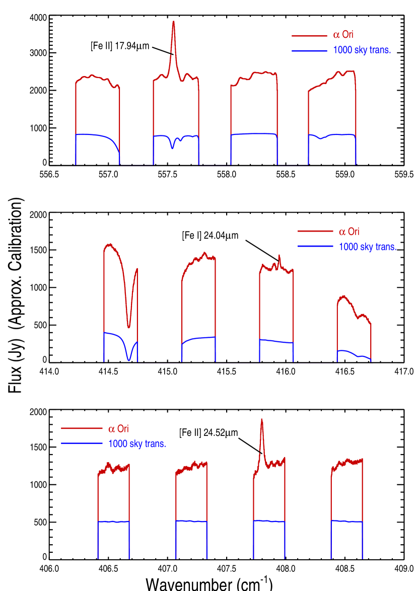
Figure 2: TEXES observations of Betelgeuse. The stellar spectra with the flux calibration described in Appendix A are shown in red. An estimate of the sky transmission is shown in blue. The three emission lines are clearly visible and spectrally well resolved. The [Fe II] lines are much stronger than [Fe I] because Fe II is the dominant ionization stage in the extended envelope. The telluric absorption features are used to establish a wavelength scale accurate to $<1{\rm km\>s}^{-1}$. There is a telluric water line underlying the [Fe II] 17.936 $\mu$m line, while the shapes of the [Fe II] 24.519 and [Fe I] 24.042 $\mu$m lines are not significantly affected by telluric water. The underlying stellar photosphere also has shallow molecular features that give rise to the structured continuum.

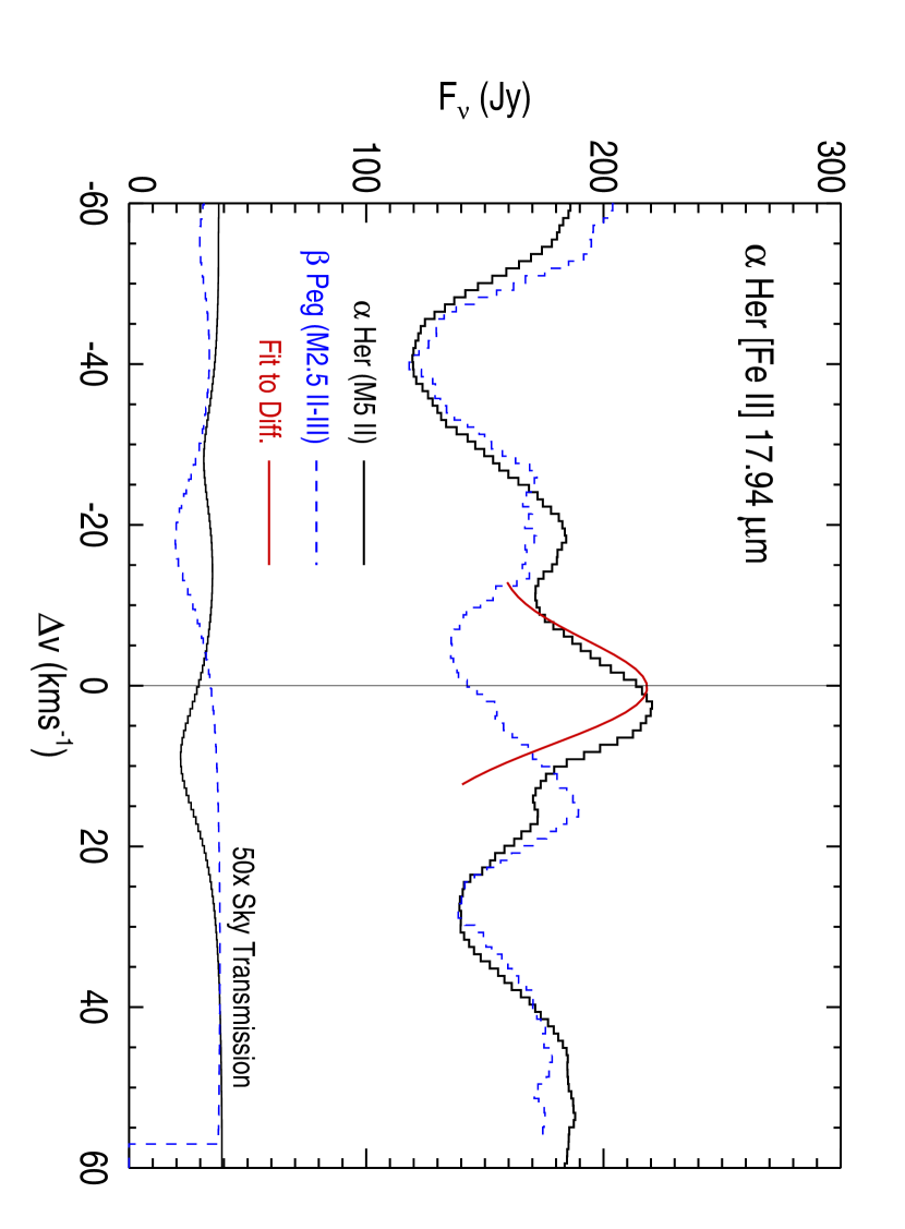
Figure 6: Identification of [Fe II] 17.94 $\mu$m emission line in $\alpha^{1}$ Her (black) while $\beta$ Peg (blue) does not show an emission feature. Subtracting the scaled $\beta$ Peg spectrum from the $\alpha^{1}$ Her that has been flat-fielded with NML Cyg reveals emission at the rest wavelength of $\alpha^{1}$ Her. A Gaussian fit to this difference spectrum is shown in red and the properties are given in Table 3. The sky transmission for these two stars is also shown and significant additional uncertainties resulting from the combined telluric correction are expected. Subsequent observations of the 24.52 $\mu$m line have confirmed this detection of [Fe II]. A color version of this figure is available in the electronic edition.

Table 1: Radiative Atomic Data for Diagnostic Infrared [Fe II] lines.

Species	Wavelength	Wavenumber	$E_{low}\>\>\>\>$	$J_{low}$	$E_{up}\>\>\>\>$	$J_{up}$	$A_{ji}$
	($\mu$m)	$({\rm cm}^{-1})$	$({\rm cm}^{-1})$		$({\rm cm}^{-1})$		$({\rm s}^{-1})$
TEXES
[Fe II]	17.9360	557.5364	1872.6005	9/2	2430.1369	7/2	$5.84\times 10^{-3}$
[Fe II]	24.5192	407.8434	2430.1369	7/2	2837.9803	5/2	$3.92\times 10^{-3}$
ISO
[Fe II]	25.9884	384.7868	0.0000	9/2	384.7868	7/2	$2.13\times 10^{-3}$
[Fe II]	35.3486	282.8963	384.7868	7/2	667.6830	5/2	$1.57\times 10^{-3}$

Table 2: TEXES [Fe II] and [Fe I] Observation Summary for 2004 October 5,6,11, 2005 January 16,17, and 2005 December 9.

Star	Spectral-Type	$V_{rad}$	[FeII] 17.94	[FeII] 24.52	[FeI] 24.04
		(${\rm km\>s}^{-1}$)	($\mu$m)	($\mu$m)	($\mu$m)
$\mu$ Cep	M2 Ia	+19.4	$\surd$	$\surd$	-
$\alpha$ Sco	M1 Iab	-3.5	-	$\surd$	-
$\alpha$ Ori	M2 Iab	+20.7	$\surd$	$\surd$	$\surd$
CE Tau	M2 Iab	+22.8	$\surd$	$\surd$	-
AD Per	M2.5 Iab	-44	$\surd$	-	-
$\alpha$ Her	M5 II	-33.1	$\surd$	-	X
$\beta$ Peg	M2.5 II-III	+9.1	X	-	-
Mira	M7 III	+63.5	X	X	-
$\zeta$ Aur	K4 Ib-II	Binary	X	-	-
$\alpha$ Tau	K5 III	+54.3	X	X	-

Table 3: Line Centroid Velocities and Doppler Widths ($\pm 1\sigma$) of the [Fe II] Emission Lines.

Star	Spectral-Type	$V_{rad}$	$V_{cent}$	$V_{Dopp}$(Obs)
		(${\rm km\>s}^{-1}$)	(${\rm km\>s}^{-1}$)	(${\rm km\>s}^{-1}$)
$\mu$ Cep	M2 Ia	+19.4	$1.7\pm 0.2$	$13.4\pm 0.4$
$\alpha$ Sco	M1 Iab	-3.5	No WaveCal	$15.6\pm 0.3$
$\alpha$ Ori	M2 Iab	+20.7	$0.0\pm 0.6$	$12.5\pm 0.8$
CE Tau	M2 Iab	+22.8	$0.0\pm 0.1$	$12.0\pm 0.2$
AD Per	M2.5 Iab	-44	$2.0\pm 1.5$	$14.4\pm 1.4$
$\alpha$ Her	M5 II	-33.1	$1.7\pm 0.5$	$9.2\pm 0.8$

Table 4: Properties of $\alpha$ Ori’s TEXES [Fe II] emission lines.

Date	Flux	$V_{cent}$	$V_{Dopp}$(Obs)
UT	($10^{-19}\>{\rm W\>cm}^{-2}$)	(${\rm km\>s}^{-1}$)	(${\rm km\>s}^{-1}$)
Fe II 24.52 $\mu$m
2004 Oct 05	$6.2\pm 0.1$	No WaveCal	$13.2\pm 0.2$
2004 Oct 06	$6.2\pm 0.2$	No WaveCal	$12.4\pm 0.5$
2004 Oct 11	$5.7\pm 0.1$	$+0.7\pm 0.1$	$12.8\pm 0.3$
2005 Jan 16	$6.0\pm 0.1$	$-1.0\pm 0.1$	$13.3\pm 0.3$
2005 Dec 09	$6.0\pm 0.1$	$-0.4\pm 0.1$	$12.9\pm 0.2$
Fe II 17.94 $\mu$m
2004 Oct 05	$16.5\pm 0.5$	$0.8\pm 0.2$	$12.0\pm 0.4$
2005 Jan 16	$16.1\pm 0.1$	$0.3\pm 0.1$	$11.7\pm 0.1$
2005 Dec 07	$16.0\pm 0.2$	$0.6\pm 0.1$	$11.4\pm 0.2$
Fe I 24.04 $\mu$m
2004 Oct 06	$0.77\pm 0.03$	$-2.7\pm 0.2$	$6.5\pm 0.3$

Table 5: Properties of Betelgeuse’s Infrared [Fe I] and [Fe II] lines.

Ion	Wavelength	$V_{cent}$	$V_{turb}$	Flux	Flux (model)
	(Vac. $\mu$m)	$({\rm km\>s}^{-1})$	$({\rm km\>s}^{-1})$	$({\rm W\>cm}^{-2})$	$({\rm W\>cm}^{-2})$
TEXES
[Fe II]	17.9360	$+0.5\pm 0.2$	$12\pm 0.1$	$1.6\pm 0.1\times 10^{-18}$	$5.4\times 10^{-18}$
[Fe II]	24.5192	$+0.0\pm 0.4$	$13\pm 0.2$	$5.9\pm 0.2\times 10^{-19}$	$1.8\times 10^{-18}$
[Fe I]	24.0423	$-2.7\pm 0.2$	$6.5\pm 0.4$	$7.7\pm 0.3\times 10^{-20}$	$7.4\times 10^{-20}$
ISO
[Fe II]	25.9884	unresolved		$2.8\pm 0.1\times 10^{-18}$	$4.4\times 10^{-18}$
[Fe II]	35.3486	unresolved		$8.3\pm 0.3\times 10^{-19}$	$1.4\times 10^{-18}$
[Fe I]	34.7133	unresolved		$<5\times 10^{-20}$	$2.2\times 10^{-20}$

Table 6: OVRO 100 GHz Radio fluxes for $\alpha$ Sco, $\alpha$ Ori, and $\alpha$ Her.

	$\alpha$ Sco	$\alpha$ Ori	$\alpha$ Her
Date	2004 Mar 30	2003 Nov 9	2004 Mar 30
Exposure Time (Hour)	2	2	5
$\alpha$ (J2000)	16h 29′  24.492″	5h 55′  10.322″	17h 14′  38.862″
$\sigma$($\alpha$)	$\pm$ 0.002″	$\pm$ 0.005″	$\pm$ 0.002″
$\delta$ (J2000)	$-26\arcdeg$ 25′  54.676″	$7\arcdeg$ 24′  25.302″	$14\arcdeg$ 23′  25.611″
$\sigma$($\delta$)	$\pm$ 0.005″	$\pm$ 0.034″	$\pm$ 0.002″
Antenna Configuration	E	L	E
Beam Size, Position Angle	$8.6\times 4.3$″, $-4.0\arcdeg$	$15.4\times 5.0$″, $-11.0\arcdeg$	$4.9\times 4.1$″, $+75.8\arcdeg$
100 GHz Flux & 1$\sigma$ (mJy)	$70\pm 1.8$	$80.4\pm 3.7$	$19\pm 0.49$
250 GHz Flux & 1$\sigma$ (mJy)	$345\pm 34$	$351\pm 25$	$104\pm 10$

Table 7: Atomic Data for CSE emission lines, and adopted abundances for $\alpha$ Ori.

Transition	Wavelength	$A_{ji}$	Abundance	$E_{up}$	Source for Abundance
	($\mu$m)	(${\rm s}^{-1}$)	(Rel. to H)	$({\rm cm}^{-1})$
[Fe I]	24.04	2.51d-03	3.0d-05	415.933	Carr et al. (2000)
[Fe II]	25.99	2.13d-03	3.0d-05	384.790	Carr et al. (2000)
[Fe II]	35.35	1.57d-03	3.0d-05	667.683	Carr et al. (2000)
[O I]	63.18	8.91d-05	6.3d-04	158.265	Lambert et al. (1984)
[O I]	145.5	1.75d-05	6.3d-04	226.977	Lambert et al. (1984)
[Si II]	34.81	2.13d-04	3.8d-05	287.24	Rodgers & Glassgold (1991)
[C I]	609.7	7.88d-08	2.5d-04	16.40	Lambert et al. (1984)
[C II]	157.7	2.30d-06	2.5d-04	63.42	Lambert et al. (1984)

Table 8: Other observed forbidden line fluxes for $\alpha$ Ori and computed flxues from the Composite Model Atmosphere described in Appendix B.

Transition	Flux (observed)	Flux (model)	Reference for Observed Fluxes
	$({\rm W\>cm}^{-2})$	$({\rm W\>cm}^{-2})$
[O I] 63.18 $\mu$m	$2.4\pm 0.2\times 10^{-18}$	$8.9\times 10^{-19}$	Haas & Glassgold (1993)
	$1.1\pm 0.2\times 10^{-18}$		Haas et al. (1995)
	$1.9\pm 0.1\times 10^{-18}$		ISO Castro-Carrizo et al. (2001)
[O I] 145.5 $\mu$m	$11\pm 4\times 10^{-20}$	$4.8\times 10^{-20}$	Haas et al. (1995)
	$2.7\pm 0.5\times 10^{-20}$		Castro-Carrizo et al. (2001)
	$5\times 10^{-20}$		Barlow (1999) (& Priv. Comm)
[Si II] 34.81 $\mu$m	$0.93\pm 0.08\times 10^{-18}$	$1.5\times 10^{-18}$	ISO This paper
	$0.94\pm 0.37\times 10^{-18}$		Haas & Glassgold (1993)
[C II] 157.7 $\mu$m	$1.1\pm 0.1\times 10^{-19}$	$0.7\times 10^{-19}$	Barlow (1999)
	$1.2\pm 0.1\times 10^{-19}$		Castro-Carrizo et al. (2001)

Appendix A Approximate Absolute Flux Calibration for the TEXES $\alpha$ Ori Spectra

The analysis of M supergiant atmospheric dynamics can be made without an absolute flux calibration of the TEXES spectra, but to explore the full thermodynamic diagnostic potential of the [Fe II] 24.52 $\mu$m and 17.94 $\mu$m, and [Fe I] 24.04 $\mu$m emission lines requires absolute flux calibrated spectra. This enables a comparison of flux predictions from model atmospheres with observations from airborne and space observatories, i.e., [Si II] and [O I] emission detected with KAO, and [C II] and [Fe II] emission in ISO spectra. Here we describe an approximate flux calibration of the TEXES spectra for $\alpha$ Ori which has several independent mid-IR flux measurements that can be used to calibrate and correct for the TEXES slit losses.

In this Appendix we bring the TEXES spectra to an absolute scale by adopting the shape of published ISO Short Wavelength Spectrometer (SWS) spectra over the 16.5-26.5 $\mu$m wavelength region and scale the continuum flux at 25 $\mu$m to a value derived from a combination of fluxes from color-corrected photometry from the Diffuse Infrared Background Experiment (DIRBE) on the Cosmic Background Explorer (COBE) satellite (Boggess et al., 1992), color-corrected InfraRed Astronomical Satellite (IRAS) photometry, and the cryogenic grating spectrometer (CGS) on the KAO (Haas & Glassgold, 1993). These are also checked against 8-13 $\mu$m UKIRT CGS3 spectrophotometry (Monnier et al., 1998).

$\alpha$ Ori’s mid-IR spectra contains emission from close to the star and from spatially extended optically thin silicate dust emission. The TEXES, ISO, IRAS, KAO-CGS, and DIRBE observations all have different entrance apertures and beam sizes and as a consequence the TEXES spectra are scaled with differential corrections that account for the different TEXES slit losses for the extended dust and point source stellar emission. The individual steps are outlined below.

A.1 ISO Spectrometers

To derive color-corrected fluxes for the DIRBE and IRAS photometry the spectral shape and system responses are required across each photometric passband. To find the color-corrections $K_{\lambda}$, where the observed color-corrected flux is given by $F_{obs}=F_{DIRBE,IRAS}/K_{\lambda}$, we adopted ISO spectra and MARCS models (see Table 9).

Three different reductions of $\alpha$ Ori’s ISO SWS spectra, obtained with a grating resolution of $R\sim 1000$ at scan speed #4, from Justtanont et al. (1999), Verhoelst et al. (2006), and Sloan et al. (2003) were used to derive $K_{\lambda}$ for the DIRBE 3.5 $\mu$m, 4.9 $\mu$m, 12 $\mu$m, and 25 $\mu$m and IRAS 12, and 25 $\mu$m fluxes. The LWS grating spectrum which was obtained two days before the end of the ISO mission (Barlow, 1999) was used to find $K_{\lambda}$ for the 60 and 100 $\mu$m fluxes.

The [Fe II] TEXES observations correspond to the ISO SWS band 3 which has a $14\times 27\arcsec$ aperture. Betelgeuse is a bright IR source and provides an ISO calibration challenge in addition to ISO’s known systematic flux calibration errors (Verhoelst et al., 2006). This is a reason why the published flux spectrum values differ by as much as 40%. In the following we boot-strap the ISO flux calibration using the color-corrected photometry.

A.2 DIRBE Photometry

We processed the DIRBE photometry from the Calibrated Individual Observations in a fashion similar to Smith (2003) and Smith et al. (2004). Flux outliers caused by cosmic rays coincident with, and off, the source position were rejected. We did not use IR databases to reject certain scan directions to avoid potential source confusion which can be important at shorter wavelengths. The color-uncorrected fluxes are given in Table 9. These are essentially identical to those found by Smith (2003) and Smith et al. (2004). There are typically about 300 measurements in each band.

At 25 $\mu$m and 60 $\mu$m the mean of the individual flux error estimates is similar to the $1\sigma$ standard deviation of the total dataset, while at 12 $\mu$m the $1\sigma$ standard deviation is three times the mean error hinting at intrinsic short term variability during this epoch. Over the 10 months of cryogenic DIRBE observations there was a 7% increase in flux at 12 $\mu$m and a 3% increase at 25 $\mu$m. Note that the standard deviation of the mean is an order of magnitude smaller than the standard deviation of the individual measurements.

To convert the DIRBE photometry into color-corrected fluxes the spectral distributions across each band were combined with the spectral response curves from Hauser et al. (1998). The color-corrected fluxes are given in Table 9

A.3 IRAS Photometry and Low Resolution Spectrometer

Betelgeuse had IRAS 12, 25, 60, and 100 $\mu$m fluxes measured three times in March 1983 and the differences in the individual measurements were consistent with their uncertainties. The IRAS Point Source Catalog measurements are given in Table 9.

The IRAS Low Resolution Spectrometer (LRS) spectra have a resolution of $R\sim 20$ and cover 7.5-22.5 $\mu$m. The $\alpha$ Ori LRS spectra were combined with the correction factors from Cohen et al. (1992) and the system responses from the IRAS Explanatory Supplement (1988) to derive a color-corrected 12 $\mu$m flux of $3393\pm 136$ Jy. For the 25, 60 and 100 $\mu$m fluxes we used the non-contemporaneous ISO SWS and LWS spectral shape to derive color-corrected fluxes which are given in Table 9.

A.4 Kuiper Airborne Observatory

Haas & Glassgold (1993) report the 1992 January 16 detection of [Si II] 34.81 $\mu$m and [O I] 63.18 $\mu$m emission lines using the cryogenic grating spectrometer (CGS) on-board the KAO with resolutions of $R\simeq 2900$ (44″  aperture) and $R\simeq 3700$ (34″  aperture), respectively. The measured line fluxes are: [Si II] $=0.94\pm 0.37\times 10^{-18}\>{\rm W\>cm}^{-2}$ and [O I] $=2.37\pm 0.21\times 10^{-18}\>{\rm W\>cm}^{-2}$. They also measured nearby continuum fluxes of $724\pm 29$ Jy at 35 $\mu$m, and $96\pm 41$ Jy at 63 $\mu$m.

Table 9: DIRBE and IRAS photometry: color-uncorrected and color-corrected flxues.

Band	Wavelength	Color-Uncorrected	Color-Corrected	$K_{\lambda}\>$ Spectral shape
	($\mu$m)	Flux $\pm 1\sigma$ (Jy)	Flux $\pm 1\sigma$ (Jy)
DIRBE
Band 1	1.25	$3.04\pm 0.11\times 10^{4}$	$3.20\pm 0.12\times 10^{4}$	0.95 MARCS
Band 2	2.2	$3.03\pm 0.09\times 10^{4}$	$3.62\pm 0.10\times 10^{4}$	0.88 MARCS
Band 3	3.5	$1.71\pm 0.05\times 10^{4}$	$1.78\pm 0.05\times 10^{4}$	0.96 ISO-SWS
Band 4	4.9	$7.16\pm 0.31\times 10^{3}$	$7.46\pm 0.32\times 10^{3}$	0.96 ISO-SWS
Band 5	12	$3.86\pm 0.14\times 10^{3}$	$3.68\pm 0.16\times 10^{3}$	1.03 ISO-SWS
Band 6	25	$2.91\pm 0.06\times 10^{3}$	$1.48\pm 0.04\times 10^{3}$	1.95 ISO-SWS
Band 7	60	$6.29\pm 1.02\times 10^{2}$	$4.31\pm 0.70\times 10^{2}$	1.46 ISO-LWS
Band 8	100	$1.02\pm 2.76\times 10^{2}$	$0.87\pm 2.36\times 10^{2}$	1.17 ISO-LWS
IRAS
	12	$4.68\pm 0.19\times 10^{3}$	$3.39\pm 0.14\times 10^{3}$	1.38 IRAS LRS
			$3.87\pm 0.16\times 10^{3}$	1.21 ISO-SWS
	25	$1.74\pm 0.07\times 10^{3}$	$1.20\pm 0.05\times 10^{3}$	1.45 ISO-SWS
	60	$2.99\pm 0.21\times 10^{2}$	$2.23\pm 0.16\times 10^{2}$	1.34 ISO-LWS
	100	$9.59\pm 1.92\times 10^{1}$	$9.13\pm 1.83\times 10^{1}$	1.05 ISO-LWS

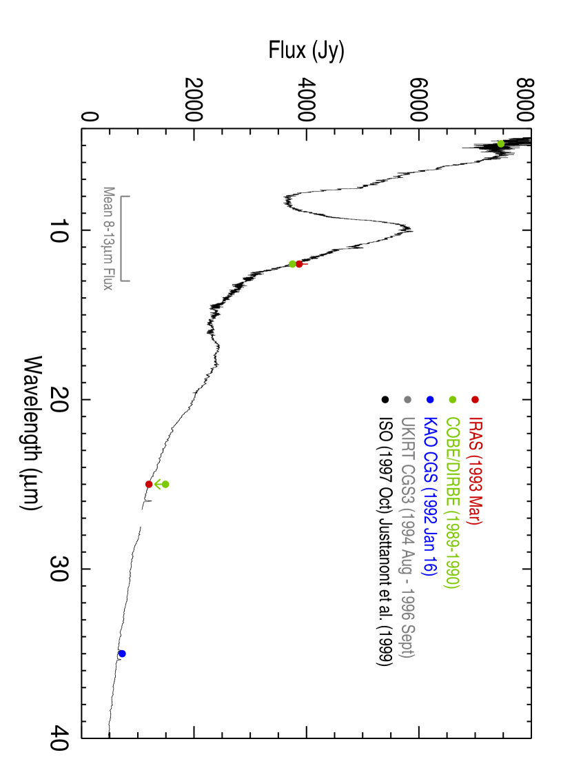
Figure 9: ISO spectra and photometry of $\alpha$ Ori described in Appendix A. The $1\sigma$ error bars are mostly within the filled circles. The flux curve of Justtanont et al. (1999) is in good agreement with the IRAS fluxes and the DIRBE 4.9 and 12 $\mu$m fluxes. The DIRBE 25 and 60 $\mu$m fluxes are upper-limits because of the large beam size and the presence of extended IR emission surrounding Betelgeuse. The KAO $3\sigma$ absolute flux uncertainty is 25% (Haas & Glassgold, 1993). We note that the calibration of Verhoelst et al. (2006) appears systematically low ($>20$%) at these wavelengths, but these authors note that their adopted multiplicative factors are lower than typically adopted. The mean 8-13 $\mu$m fluxes from UKIRT CGS3 spectrophotometry between 1994 Aug and 1996 Sept (Monnier et al., 1998) ranged from 4602-4943 Jy with 10% uncertainty in the absolute flux calibration. The mean 1997 8-13 $\mu$m value derived from Justtanont et al. (1999) is 10% lower at 4386 Jy. A color version of this figure is available in the electronic edition.

A.5 Adopted Fluxes

The IR observations discussed above were made at different epochs and stellar variability is an important consideration. Monnier et al. (1998) present seven mean 8-13 $\mu$m fluxes obtained between 1994 August and 1996 September and the variation of these fluxes were within the absolute flux calibration uncertainties of 5-10%. In the mid-1990’s there is a hint that the 9.7 $\mu$m silicate emission feature shifted slightly to shorter wavelengths than in the 1983 IRAS LRS spectra (Monnier et al., 1999). These authors also found that the LRS spectra are somewhat bluer than both previous and later observations, indicating a residual miscalibration of the IRAS LRS spectra. In light of this we redetermined the color-correction for the IRAS 12 $\mu$m flux (also given in Table 9) using the ISO-SWS spectra and this leads to a 15% difference. Bester et al. (1996) give eight 11.15 $\mu$m fluxes obtained between 1989 November and 1995 August and the variations of these are also consistent with a 5% uncertainty. Although the observations are scarce, it appears that intrinsic star+dust flux variations at 12 $\mu$m on decadal timescales are less than 10%, and at 25 $\mu$m probably less.

The DIRBE 25 $\mu$m and 60 $\mu$m fluxes from 1989-1990 are significantly larger than the 1983 IRAS fluxes, and the 25$\mu$m fluxes are greater than the Verhoelst et al. (2006) reduction of the 1997 ISO observations, which is expected to have a typical photometric uncertainty of $\sim 10$% (Van Malderen et al., 2004).

The majority of the stellar wind dust emission at 25 $\mu$m is expected to lie within $1\arcmin$ of $\alpha$ Ori (Stencel, Pesce & Hagen Bauer, 1988), i.e., well within the large DIRBE beam of $0.\arcdeg 7\times 0.\arcdeg 7$ and the IRAS detectors FOV $0.75\times 4.6\arcmin$. Only a few percent of dust emission is not collected in the ISO band 3C and 3D apertures. Noriega-Crespo et al. (1997) discovered a wind-ISM bowshock located at 5′ from the star, and a nearby linear structure. The DIRBE fluxes contain contributions from this low surface intensity structured emission. At 60 $\mu$m the bowshock alone has $\sim 30$% of the flux from the star+wind. The DIRBE color-corrected 60 $\mu$m flux $\simeq 445$ Jy is greater than the combined star+bowshock flux (Noriega-Crespo et al., 1997) and while the relative contribution of the extended emission at 25 $\mu$m is likely to be less than that at 60 $\mu$m it probably accounts for some of the excess DIRBE 25 $\mu$m flux. At 12 $\mu$m the DIRBE flux should be dominated by the star and its dusty wind, and is consistent with the IRAS flux. So although the DIRBE absolute photometry is very good, the large beam size makes it less suitable to normalize the ISO spectra for $\lambda>12\,\mu$m.

A comparison of the 4.9 and 12 $\mu$m DIRBE, the 12 and 25 $\mu$m IRAS, and the 35 $\mu$m KAO fluxes with the different ISO reductions reveals a good overall agreement with Justtanont et al. (1999) but not the Verhoelst et al. (2006) spectrum which is significantly lower. Indeed Verhoelst et al. (2006) noted that they scaled the sub-band fluxes down significantly more than expected for $\lambda>4\,\mu$m. Our results suggest that the ISO calibration for bright IR sources requires improvement.

In summary, for the absolute flux scaling of the TEXES spectra we adopt the ISO SWS spectrum normalized to the mean of the 12 & 25 $\mu$m IRAS fluxes and the 4.9 and 12 $\mu$m DIRBE fluxes. We assign an absolute flux uncertainty of 20% to account for the combined stellar variability and the scatter in the different mission normalizations. The ISO spectra scaled to these fluxes is shown in Figure 9.

The relative fluxes for the TEXES [Fe II] lines ultimately relies on the normalization of the slightly overlapping ISO spectra in band 3C ($\lambda=16.5-19.5\>\mu$m) and band 3D ($\lambda=19.5-27.3\>\mu$m), e.g., between ($\lambda 19.37-19.57\>\mu$m) (Sloan et al., 2003). The difference in the band 3C and band 3D multiplicative factors listed by Verhoelst et al. (2006) is $\simeq 1.3\%$, we therefore adopt a 2% relative flux error in the continua near the [Fe II] 17.98 $\mu$m and 24.52 $\mu$m lines.

A.6 Putting it all together

The inner dust radius is measured to be $\sim 1$″ (Danchi et al., 1994) and is comparable to the TEXES slit width in the dispersion direction. The observed TEXES spectra thus suffer different slit losses for the point source photospheric and chromospheric emission and for the more diffuse extended dust continuum emission. To place the TEXES spectra onto an absolute flux scale we must first apply corrections for the emission not transmitted through the $2\times 17\arcsec$ slit and telescope and instrument losses. To estimate the separate slit losses of star and dust we use the silicate dust specific intensity model from HBL01 and convolve the resulting sky-image with a Gaussian to represent a combination of seeing, diffraction and pointing jitter, whose width is estimated by the recorded TEXES spatial profile: FWHM$\sim 2.6\arcsec$ at 24.5 $\mu$m, and FWHM$\sim 2.1\arcsec$ at 17.9 $\mu$m.

The flux recorded by TEXES

$$F_{TEXES}=A_{loss}\left[C_{\ast}F_{\ast}+C_{dust}F_{dust}\right]$$ (A1)

where $A_{loss}$ is a multiplicative factor to account for combined telescope and instrument light losses not already corrected for in the radiometric flat-field procedure, and $C_{\ast}$ and $C_{dust}$ are the fractions of the total star and dust flux that pass through the slit, respectively. These are calculated assuming the HBL01 sky intensity model, i.e., at 24.5 $\mu$m: $C_{\ast}=0.65$ and $C_{dust}=0.31$.

We assume that the ISO aperture records the total flux from the system, i.e., the star and wind emission but not the bowshock emission then

$$F=F_{\ast}+F_{dust}.$$ (A2)

At 24.5 $\mu$m, 17.9 $\mu$m and 11.15 $\mu$m the ratio of dust to star emission derived from the HBL01 model is $F_{dust}/F_{\ast}=1.6,1.4,0.7$, respectively. Coefficients $A_{loss}$ can then be found and the TEXES spectra corrected and scaled to the ISO spectrum (which is scaled to the DIRBE and IRAS fluxes) using the four TEXES orders recorded at each wavelength setting. The resulting TEXES spectra for $\alpha$ Ori are shown in Fig. 2.

We note that the $6\arcsec$ nod of the star along the slit followed by a subtracted image which cancels the sky noise clips some of the dust emission which is present at $3\arcsec$. The spatial profile shows some emission beyond the Gaussian core and this is also predicted from the HBL01 dust model. While this does not affect the present emission line analysis we estimate that the flux measurement procedure underestimates the total flux by $\sim 5-8\%$.

Appendix B Composite Model Atmosphere

To determine the formation radii of Betelgeuse’s mid- and far-IR emission lines discussed in §5 requires a comprehensive model that encompasses the chromosphere, inner wind, and CSE. Currently no such comprehensive models exist. Models do exist for the inner region, (HBL01: Harper et al. 2001), and the CSE (RG91: Rodgers & Glassgold 1991), and here we describe a composite dynamic and thermodynamic 1-D model that utilized these models, and interpolates between them.

The HBL01 model was based on the Hipparcos $\alpha$ Ori distance of 131 pc, but fortuitously the revised distance of $197\pm 45$ pc (Harper et al., 2008) is also that originally adopted in RG91 (200 pc). We therefore take Rodger & Glassgold’s stellar parameters as our nominal values: $R_{\ast}=1078\,R_{\odot}$, and $\phi_{\ast}=50$ mas. In Harper et al. (2001) the Infrared Spatial Interferometer 11.15 $\mu$m angular diameter of 56 mas (Bester et al., 1996) was adopted, but it now appears that this may be an over-estimate of the photospheric size (Perrin et al., 2007) and the RG91 value is probably closer to the actual value.

B.1 Thermal Structure

The HBL01 model was based on angular resolved radio emission and the old Hipparcos distance of 131 pc. Although this model is insensitive to the uncertain angular diameter of the photosphere, the thermodynamic properties must be scaled to the improved distance estimate of 197 pc (Harper et al., 2008). The radio interferometry of Lim et al. (1998) essentially measures the angular distribution of the specific intensity.

If we consider the model in terms of the normalized radial distance $Z$, where $R=ZR_{\ast}$, then $T_{gas}(Z)$ remains unchanged but $R_{\ast}$ is now a factor of 197/131 larger. The angular radio brightness distribution also requires that the optical depth through the atmosphere remains unchanged, so that $\tau\propto n_{e}n_{H}dR$ is constant. Therefore to satisfy this constraint the particle densities each scale as $1/\sqrt{197/131}$.

The single component 1-D temperature structure derived from the radio represents a complicated averaging of the electron temperatures of the hot chromospheric plasma and cool wind plasma. We expect that the filling factor of the hot plasma decreases with increasing radius, so the bulk of the plasma is cooler than inferred from the radio. For the calculation of the mid-IR emission we adopt a lower temperature distribution that joins the HBL01 model at $Z=7$.

When the RG91 models were constructed it was widely believed, on the basis of theoretical grounds and semi-empirical models based on spatially unresolved data, that the inner wind had warm chromospheric temperatures and RG91 adopted a nominal inner boundary condition (BC) of $T_{gas}=8000$ K at $Z=3$. They also provided variational calculations for the temperature structures resulting from different mass-loss rates and where the inner BC was set to $T_{gas}=4000$ K. In contrast $T_{gas}=2764$ K for HBL01. The RG91 models with different inner temperature BC’s have similar shapes and smoothly converge to join at 30$R_{\ast}$. Interior to $Z=7$ we take the temperature structure from HBL01 which is constrained by the long-wavelength radio observations, and exterior to that the temperature structure is obtained by extrapolating on the difference between the RG91 models with inner BC of $T_{e}=4000$ K and 10,000 K.

The CSE temperature structures are less sensitive to differences in mass-loss rates: the RG91 value of $3.5\times 10^{-6}\>{\rm M}_{\odot}{\rm yr}^{-1}$ (assuming a mean mass per hydrogen nuclei $\Sigma=1.4$ with $V_{wind}=10\>{\rm km\>s}^{-1}$) is similar to the rescaled value of HBL01 (see below). The adopted composite temperature structures are shown in Figure 10. The solid line includes contribution from hot plasma while the dashed line is a schematic representation of the temperature of the cool wind.

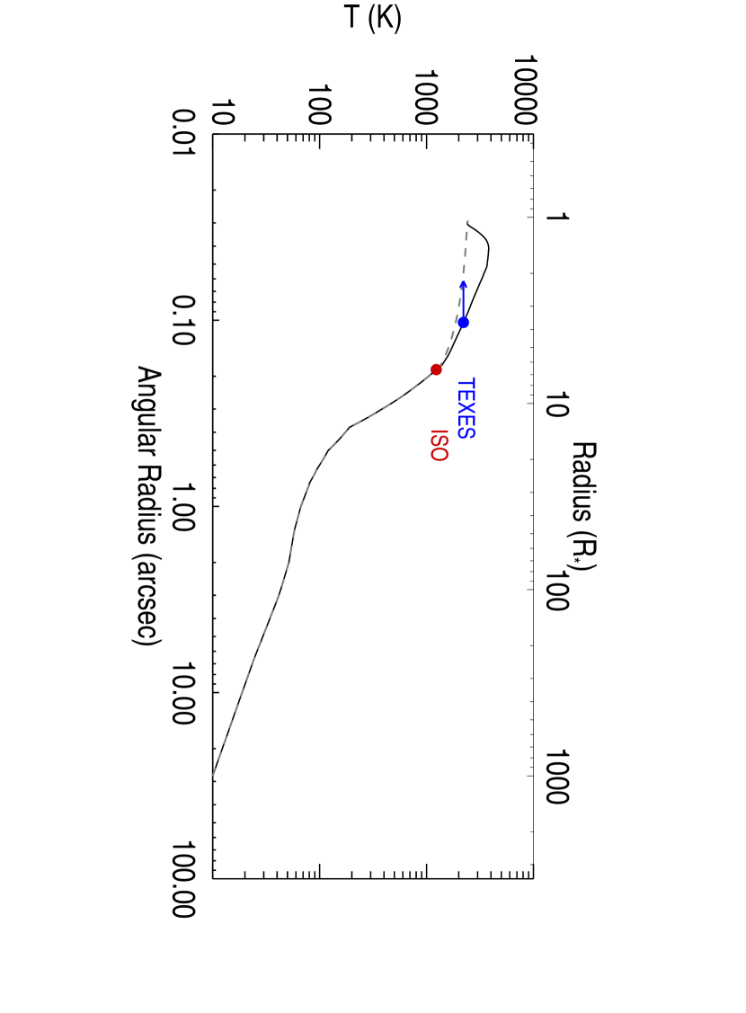
Figure 10: Composite temperature structure for $\alpha$ Ori’s chromosphere, inner wind and CSE. The inner region (solid line) is based on a distance-scaled HBL01 spatially-extended semi-empirical model, and the CSE is based on a model of Rodgers & Glassgold (1991). The dash line is a schematic representation of the temperature of the dominant plasma (see text for details.)

B.2 Velocity Fields

A detailed description of the run of the mean outflow velocity, $V(R)$, and fluctuations about this value, $V_{turb}(R)$, are important for both emission line profile calculations and for determining the photon escape probability which enters into the flux emitted by the envelope. $V_{turb}(R)$ which enters into the line profile calculations is assumed to be random and isotropic (in the absence of any other knowledge) and given by $V_{turb}(R)=\sqrt{V_{therm}^{2}+V_{non-therm}^{2}}$, i.e., it includes the thermal motion of the diagnostic species combined with, as yet unidentified, non-thermal motions. Here $V_{non-therm}$ dominates.

B.2.1 Mean Radial Outflow Velocity

Goldberg (1979) discussed the empirical wind velocity constraints from atomic and molecular absorption lines. There are two clearly identified velocity features and a dynamic region which may be physically distinct. The S2 shell which is narrow and discrete in velocity-space [$V_{turb}\leq 1\,{\rm km\>s}^{-1}$ and $V(S2)\simeq 17\,{\rm km\>s}^{-1}$] is observed in both absorption and scattered emission from atomic lines (Mauron, 1990), in absorption in the CO 4.6 $\mu$m fundamental band (Bernat et al., 1979), and in emission in millimeter CO rotational emission. In K I the S2 shell is seen out to a radius of 50″  (Plez & Lambert, 2002) with an inner edge of $\sim 7$″  (Mauron, 1990). However, the similarity of the shape of CO mm-radio emission profile in single-dish observations with different beam-sizes suggests the outer edge of the CO is $<12$″, e.g., Huggins et al. (1994), and from modeling considerations an inner edge of 2.5″  is plausible (Huggins, 1987). The spatial extent of different diagnostics is unlikely to be identical because of differing ionization balances in the extended envelope. We shall find that the atomic and singly ionized CSE emission lines are formed within these inner radii and are likely to be characteristic of the S1 shell [$V_{turb}\sim 4\,{\rm km\>s}^{-1}$ and $V(S1)\simeq 10\,{\rm km\>s}^{-1}$]. S1 is observed in P-Cygni profiles and is blended with the photospheric absorption line, which may lead to a small over-estimate of the radial velocity of the shell. While S1 has not yet been spatially resolved in mm-radio CO observations, which show that it lies within the S2 shell (Harper et al., 2009), the S1 shell has been resolved in the photospheric scattered CO 4.6 $\mu$m fundamental band (Smith et al., 2009).

Dynamic flow features have been observed in ultraviolet (UV) Fe II line profiles (Boesgaard & Magnan, 1975), and Carpenter (1984) schematically mapped out the radial wind velocity using observations from the International Ultraviolet Explorer. The wind acceleration is more seen clearly in the Goddard High Resolution Spectrograph (GHRS) spectra studied by Carpenter & Robinson (1997) (see their Figure 6). The line profiles map the flows close to the star and this acceleration region may be part of S1 structure. At 1-1.5″ CO 4.6 $\mu$m wind scattering observations from Phoenix on Gemini-S (Harper et al. 2009; Smith et al. 2009) reveal that the wind has the velocity of the S1 shell. The emission for most CSE lines (except carbon) is formed interior to 1″  so we will adopt a wind model that reaches a terminal speed of $\sim 10\>{\rm km\>s}^{-1}$ at 1″ and extended out beyond 5″. Given that it is unlikely that there is a smooth transition in the wind properties between the S1 and S2 material this is a reasonable procedure, until further spatial information is obtained in this interesting region.

We estimate the run of wind velocity close to the star using the new temperature structure to locate the normalized radius $(Z)$ where the absorption minima $(V_{abs})$ of UV GHRS Fe II wind features have a radial optical depth $\tau=1$. We then select a wind velocity profile that approximates a range of Fe II $Z-V_{abs}$ values and that is also the solution to the constant pressure wind equation (Brandt, 1970),

$${V^{2}\over{V_{crit}^{2}}}-\ln{V^{2}\over{V_{crit}^{2}}}=4\left[\ln{R\over{R_{crit}}}+{R_{crit}\over{R}}\right]-3.$$ (B1)

The velocity profile is the solution of this transcendental equation, and is defined by $V_{crit}=2.5\>{\rm km\>s}^{-1}$ and $Z_{crit}=2.75$. We also limit the wind speed not to exceed $10\>{\rm km\>s}^{-1}$ at large distance.

B.2.2 Turbulence Velocities

For the radial distribution of turbulence, we note that the studies of eclipsing binaries reveal that the turbulent velocities in the chromosphere and inner wind are typically $\simeq 1.5\times$ hydrogen sound speed (Eaton 1993; Baade et al. 1996), but see also Kirsch et al. (2001). These small scale motions are probably related to the mass-loss mechanisms and may reflect MHD waves, e.g., see Jordan (1986). Here we adopt $\simeq 1.5\times$ hydrogen sound speed, namely

$$V_{non-therm}\left(R\right)=0.19\sqrt{T_{gas}\left(R\right)}\>\>{\rm km\>s}^{-1}.$$ (B2)

We note that this gives $V_{turb}\simeq V_{non-therm}\sim 12\>{\rm km\>s}^{-1}$ near the base of the wind in agreement with $\alpha$ Ori’s [Fe II] line widths. In this model at $Z\simeq 9$ the wind and non-thermal turbulence velocities are approximately equal.

B.3 Density Structure

For the hydrogen densities we join the distance-scaled HBL01 model with the RG91 model. The densities in the RG91 model are $\propto\dot{M}/V_{\infty}$ and they originally adopted a terminal wind speed of $V_{\infty}=16\>{\rm km\>s}^{-1}$ (i.e., the S2 velocity), however, it now appears that the appropriate wind speed for the most of the CSE line formation is $10\>{\rm km\>s}^{-1}$ (Haas & Glassgold, 1993). To maintain the same density structure with this lower velocity requires lowering the original RG91 mass-loss rate of $\dot{M}=5.6\times 10^{-6}\>{\rm M}_{\odot}{\rm yr}^{-1}$ to $\dot{M}=3.5\times 10^{-6}\>{\rm M}_{\odot}{\rm yr}^{-1}$. We define the hydrogen density for $Z>7$ assuming

$$n_{H}={\dot{M}\over{4\pi R^{2}m_{H}\Sigma V(R)}}.$$ (B3)

The densities are therefore increased over the constant wind velocity limit. At $Z=7$ the inner densities are a factor $\sim 2$ larger than implied by Eq B3 so the two have a simple join. The mass-loss rate implied by the UV Fe II lines with this new density structure is $4.8\pm 1.3\times 10^{-6}\,{\rm M}_{\odot}{\rm yr}^{-1}$ which is consistent with the lower velocity RG91 value.

B.4 Inhomogeneities

The 1-D thermal structure derived from radio interferometry represents a mean value of the different structures that co-exist at a given stellar radius. Near the temperature peak a crude estimate gives an area filling factor of hot chromospheric material of $A_{chrom}\left(Z\right)\sim 1/3$ (Harper et al., 2001), while by $Z\sim 3$ the filling factor is much smaller (Harper & Brown, 2006). The filling factor of the hot plasma is expected to continue to decrease with increasing radius. The temperature of the bulk plasma in the region that encompasses the hot chromosphere might then be lower than the HB01 model, and an alternate schematic model is shown as a dash line in Fig. 10, and this is adopted in §5 to calculate the contribution functions.

References

- Aannestad (1973) Aannestad, P. 1973, ApJS, 25, 223
- Airapetian etal. (2000) Airapetian, V. S., Ofman, L., Robinson, R. D., Carpenter, K. G., & Davila, J. 2000, ApJ, 528, 965
- Aldenius & Johansson (2007) Aldenius, M. & Johansson, S. 2007, A&A, 467, 753
- Altenhoff et al. (1994) Altenhoff, W. J., Thum, C., & Wendker, H. J. 1994, A&A, 281, 161
- Aoki et al. (1998) Aoki, W., Tsuji, T., & Ohnaka, K. 1998, A&A, 333, L19
- Ayres (2002) Ayres, T. R. 2002, ApJ, 460, 1042
- Baade et al. (1996) Baade, R., Kirsch, T., Reimers, D., Toussaint, F., Bennett, P. D., Brown, A., & Harper, G. M. 1996, ApJ, 466, 979
- Bahcall & Wolf (1968) Bahcall, J. N. & Wolf, R. A. 1968, ApJ, 152, 701
- Barbier-Brossat & Fignon (2000) Barbier-Brossat, M. & Fignon, P. 2000, A&AS, 142, 217
- Barlow (1999) Barlow, M. J. 1999, IAU Symp. 191, Eds. T. Le Bertre, A. Lèbre, & C. Waelkens, p. 353
- Bernat (1981) Bernat, A. P. 1981, ApJ, 246, 184
- Bernat et al. (1979) Bernat, A. P., Hall, D. N. B., Hinkle, K. H., & Ridgway, S. T. 1979, ApJ, 233, L135
- Bester et al. (1996) Bester, M., Danchi, W. C., Hale, D., Townes, C. H., Degiacomi, C. G., Mékarnia, & Geballe, T. R. 1996, ApJ, 463, 336
- Boesgaard & Magnan (1975) Boesgaard, A. & Magnan, P. 1975, ApJ, 198, 369
- Boggess et al. (1992) Boggess, N. W., et al. 1992, ApJ, 397, 420
- Brandt (1970) Brandt, J. C., 1970, Introduction to the Solar Wind, Freeman San Franscico (p. Eq. 3.13)
- Brown & Evenson (1995) Brown, J. M. & Evenson, K. M. 1995, ApJ, 441, L97
- Carpenter (1984) Carpenter, K. G. 1984, ApJ, 285, 181
- Carpenter & Robinson (1997) Carpenter, K. G. & Robinson, R. D. 1997, ApJ, 479, 970
- Carpenter et al. (1995) Carpenter, K. G., Robinson, R. D., & Judge, P. G. 1995, ApJ, 444, 424
- Carpenter et al. (1991) Carpenter, K. G., Robinson, R. D., Wahlgren, G. M., Ake, T. B., Ebbets, D. C., Linsky, J. L., Brown, A., & Walter, F. M. 1991, ApJ, 377, L45
- Carr et al. (2000) Carr. J. S., Sellgren, K., & Balachandran, S. C. 2000, ApJ, 530, 307
- Castor (1970) Castor, J. I. 1970, MNRAS, 149, 111