Theory and optimization of transformation-based quadratic spherical cloaks

Abstract

Based on the concept of the cloak generating function, we propose a numerical method to compute the invisibility performance of various quadratic spherical cloaks and obtain optimal invisibility results. A non-ideal discrete model is used to calculate and optimize the total scattering cross-sections of different profiles of the generating function. A bell-shaped quadratic spherical cloak is found to be the best candidate, which is further optimized by controlling design parameters involved. Such improved invisibility is steady even when the model is highly discretized.

1 Introduction

Recently, great progress has been made in both the theory of and experiments on invisibility cloaks [1, 2, 3, 4]. Wide applications have been found in microwave spectrum [5, 6, 7, 8, 9, 10], optical regime [11, 12, 13, 14, 15, 16], elastodynamics [17, 18], quantum mechanics [19, 20], and acoustics [21, 22, 23, 24]. One approach to achieve an invisibility cloak is to employ the transformation optics (TO) to allow electromagnetic waves to be directed around the concealed region and smoothly recovered afterwards. The anisotropic parameters of such a cloak are derived from the coordinate transformation. This approach was generalized from the cloaking of thermal conductivity [25] and then widely applied in many other areas, which provides new approaches to conceal passive/active objects [26, 27] within their interiors invisible to external illuminations. The fundamental idea is the invariance of Maxwell’s equations under a space-deforming transformation if the material properties are altered accordingly; i.e., a specific spatial compression is equivalent to a variation of the material parameters in the flat space. Based on TO concept, many efforts have been devoted to the study of 2D cloaks (cylindrical [31], elliptical [32], and arbitrary cross-section [33]) due to the simplicity in numerical simulations. Inspired by the classic spherical cloak [1], the expressions of electromagnetic fields were explicitly presented in terms of spherical Bessel functions by Mie theory [26]. However, this analytical scattering theory for classic spherical cloaks cannot work if the anisotropic ratio (see the original definition in [34]) is anything other than that in [26]. Two solutions to overcome this problem were proposed: 1) multilayers of alternating isotropic layers [35]; and 2) discrete model of the inhomogeneous anisotropic shell, and each layer is radially anisotropic but homogeneous [36]. Then, the spherical invisibility cloak is near-perfect. Another non-TO route to the cloaking in canonical shape is to use a homogenous anisotropic [28, 29] or isotropic plasmonic [30] coating. However, in this method, the effectiveness and properties of the cloak depend on the object to be cloaked as well as that its size has to be sufficiently small compared with the wavelength. Usually, TO-based spherical cloaks need to know the prescribed transformation functions first and the required parameters can thus be obtained by constructing the explicit transformation matrices.

Certainly, those sets of parameters from various generating functions for quadratic spherical cloaks are ideal, all of which should give zero scattering theoretically. However, in actual situations, one has to consider a discrete multilayered model so that the invisibility performances of different generating functions distinguish from each other. The general method developed in [36] is adopted to calculate the far-field scattering. Our numerical results reveal that the power quadratic bell-shaped cloak yields the lowest scattering under the same discretization, which is still pronounced when the ideal cloaking shell is highly discretized.

This paper is organized as follows. Section 2 proposes the analysis method which will be used to discretize the cloaking shell into multiple layers and then compute the far-field diagrams. Section 3 addresses that the bell-shaped profile of the generating function outperforms the other including the linear one corresponding to the classic spherical cloak. Section 4 compares different profiles which give rise to bell-shaped profiles. Section 5 discusses the optimization of bell-shaped quadratic cloaks where the steady improvement in invisibility performance is verified.

2 Scattering Algorithm for Arbitrary Spherical Cloaks in Discretized Model

In this section, the scattering theory of multilayer anisotropic spherical particles is provided and applied to study a spherical cloak with arbitrary transverse and radial parameters. We suppose that the arbitrary field distribution of the incident monochromatic wave interacts with the two-layer sphere. The inner sphere is supposed to be made of isotropic material. The parameters of the coating depend on the radial coordinate and specify the rotationally symmetric anisotropy of the form

$$\varepsilon=\varepsilon_{r}(r){\bf e}_{r}\otimes{\bf e}_{r}+\varepsilon_{t}(r)I,\qquad\mu=\mu_{r}(r){\bf e}_{r}\otimes{\bf e}_{r}+\mu_{t}(r)I,$$ (1)

where $\varepsilon_{r}$ and $\mu_{r}$ are the radial dielectric permittivity and magnetic permeability, $\varepsilon_{t}$ and $\mu_{t}$ are the transversal material parameters, $I=1-{\bf e}_{r}\otimes{\bf e}_{r}={\bf e}_{\theta}\otimes{\bf e}_{\theta}+{\bf e}_{\varphi}\otimes{\bf e}_{\varphi}$ is the projection operator onto the plane perpendicular to the vector ${\bf e}_{r}$, unit vectors ${\bf e}_{r}$, ${\bf e}_{\theta}$, and ${\bf e}_{\varphi}$ are the basis vectors of the spherical coordinates.

Using the separation of the variables, the solution of Maxwell’s equations in spherical coordinates ($r$, $\theta$, $\varphi$) can be presented as

$${\bf E}(r,\theta,\varphi)=F_{lm}(\theta,\varphi){\bf E}(r),$$

$${\bf H}(r,\theta,\varphi)=F_{lm}(\theta,\varphi){\bf H}(r),$$ (2)

where the designation ${\bf E}(r)$ means that the components of the electric field vector depend only on the radial coordinate $r$ as $E_{r}(r)$, $E_{\theta}(r)$, and $E_{\varphi}(r)$ (however, the vector itself includes the angle dependence in the basis vectors), the second rank tensor in three-dimensional space $F_{lm}$ serves to separate the variables ($l$ and $m$ are the integer numbers). It can be written as the sum of dyads:

$$F_{lm}=Y_{lm}{\bf e}_{r}\otimes{\bf e}_{r}+{\bf X}_{lm}\otimes{\bf e}_{\theta}+({\bf e}_{r}\times{\bf X}_{lm})\otimes{\bf e}_{\varphi}.$$ (3)

where $Y_{lm}(\theta,\varphi)$ and ${\bf X}_{lm}(\theta,\varphi)$ are the scalar and vector spherical harmonics. Tensor functions $F_{lm}$ are very useful because of their orthogonality conditions

$$\int_{0}^{\pi}\int_{0}^{2\pi}F_{l^{\prime}m^{\prime}}^{+}(\theta,\varphi)F_{lm}(\theta,\varphi)\sin\theta{\rm d}\theta{\rm d}\varphi={\bf 1}\delta_{l^{\prime}l}\delta_{m^{\prime}m}.$$ (4)

From the commutation of the dielectric permittivity $\varepsilon$ and magnetic permeability $\mu$ tensors with $F_{lm}$ it follows that the electric and magnetic fields satisfy the system of ordinary differential equations

$${\bf e}_{r}^{\times}\frac{{\rm d}{\bf H}}{{\rm d}r}+\frac{1}{r}{\bf e}_{r}^{\times}{\bf H}-\frac{\rmi\sqrt{l(l+1)}}{r}{\bf e}_{\varphi}^{\times}{\bf H}=-\rmi k_{0}\varepsilon{\bf E},$$

$${\bf e}_{r}^{\times}\frac{{\rm d}{\bf E}}{{\rm d}r}+\frac{1}{r}{\bf e}_{r}^{\times}{\bf E}-\frac{\rmi\sqrt{l(l+1)}}{r}{\bf e}_{\varphi}^{\times}{\bf E}=\rmi k_{0}\mu{\bf H}.$$ (5)

where $k_{0}=\omega/c$ is the wavenumber in vacuum, $\omega$ is the circular frequency of the electromagnetic wave. Quantity ${\bf n}^{\times}$ is called tensor dual to the vector ${\bf n}$. It results in the vector product, if multiplied by a vector ${\bf a}$ as ${\bf n}^{\times}{\bf a}={\bf n}{\bf a}^{\times}={\bf n}\times{\bf a}$.

System (5) is the result of the variable separation in Maxwell’s equations. Eq. (5) includes two algebraic scalar equations, therefore, two field components, $H_{r}$ and $E_{r}$, can be expressed by means of the rest four components. This can be presented as the matrix link between the total fields ${\bf H}={\bf H}_{\rm t}+H_{r}{\bf e}_{r}$ and ${\bf E}={\bf E}_{\rm t}+E_{r}{\bf e}_{r}$ and their tangential components ${\bf H}_{\rm t}$ and ${\bf E}_{\rm t}$:

$$\left(\begin{array}[]{c}{\bf H}(r)\\ {\bf E}(r)\end{array}\right)=V(r)\left(\begin{array}[]{c}{\bf H}_{\rm t}(r)\\ {\bf E}_{\rm t}(r)\end{array}\right),\qquad V=\left(\begin{array}[]{cc}I&\frac{\sqrt{l(l+1)}}{\mu_{r}(r)k_{0}r}{\bf e}_{r}\otimes{\bf e}_{\theta}\\ -\frac{\sqrt{l(l+1)}}{\varepsilon_{r}(r)k_{0}r}{\bf e}_{r}\otimes{\bf e}_{\theta}&I\end{array}\right).$$ (12)

Excluding the radial components of the fields from Eq. (5), we get to the system of ordinary differential equations of the first order for the tangential components joined into the four-dimensional vector ${\bf W}(r)$ as

$$\frac{{\rm d}{\bf W}(r)}{{\rm d}r}=\rmi k_{0}M(r){\bf W}(r),$$ (13)

where

$$M=\left(\begin{array}[]{cc}A&B\\ C&D\end{array}\right),\qquad{\bf W}=\left(\begin{array}[]{c}{\bf H}_{\rm t}\\ {\bf E}_{\rm t}\end{array}\right)\equiv\left(\begin{array}[]{c}H_{\theta}\\ H_{\varphi}\\ E_{\theta}\\ E_{\varphi}\end{array}\right),$$

$$A=D=\frac{\rmi}{k_{0}r}I,\qquad B=\varepsilon_{t}{\bf e}_{r}^{\times}-\frac{l(l+1)}{\mu_{r}k_{0}^{2}r^{2}}{\bf e}_{\varphi}\otimes{\bf e}_{\theta},\qquad C=-\mu_{t}{\bf e}_{r}^{\times}+\frac{l(l+1)}{\varepsilon_{r}k_{0}^{2}r^{2}}{\bf e}_{\varphi}\otimes{\bf e}_{\theta}.$$ (14)

Tangential field components ${\bf H}_{\rm t}$ and ${\bf E}_{\rm t}$ play the important part, because they are continuous at the spherical interface. Hence, they can be used for solving the scattering problem. At first, we will analyze the situation of $r$-dependent permittivities and permeabilities, which arise for the cloak coatings of the spheres.

Excluding the $\varphi$-components of the fields from Eq. (13), we derive the differential equation of the second order for $w_{\theta}={\bf e}_{\theta}{\bf W}=(H_{\theta},E_{\theta})$:

$$w^{\prime\prime}_{\theta}+\frac{2}{r}w^{\prime}_{\theta}-\left(\begin{array}[]{cc}\frac{\varepsilon^{\prime}_{t}}{\varepsilon_{t}}&0\\ 0&\frac{\mu^{\prime}_{t}}{\mu_{t}}\end{array}\right)w^{\prime}_{\theta}+\left[k_{0}^{2}\varepsilon_{t}\mu_{t}-\frac{1}{r}\left(\begin{array}[]{cc}\frac{\varepsilon^{\prime}_{t}}{\varepsilon_{t}}&0\\ 0&\frac{\mu^{\prime}_{t}}{\mu_{t}}\end{array}\right)-\frac{l(l+1)}{r^{2}}\left(\begin{array}[]{cc}\frac{\varepsilon_{t}}{\varepsilon_{r}}&0\\ 0&\frac{\mu_{t}}{\mu_{r}}\end{array}\right)\right]w_{\theta}=0,$$ (15)

where the prime denotes the $r$-derivative. Further we will apply the condition on the medium parameters, which is usually used for the cloaks: $\varepsilon_{r}(r)=\mu_{r}(r)$ and $\varepsilon_{t}(r)=\mu_{t}(r)$. Then the equations for $H_{\theta}$ and $E_{\theta}$ coincide and can be written in the form

$$w^{\prime\prime}_{\theta}+\left(\frac{2}{r}-\frac{\varepsilon^{\prime}_{t}}{\varepsilon_{t}}\right)w^{\prime}_{\theta}+\left[k_{0}^{2}\varepsilon_{t}^{2}-\frac{\varepsilon^{\prime}_{t}}{r\varepsilon_{t}}-\frac{l(l+1)}{r^{2}}\frac{\varepsilon_{t}}{\varepsilon_{r}}\right]w_{\theta}=0.$$ (16)

This equation can be solved analytically in the very few cases. As an example, we can offer the inversely proportional transversal $\varepsilon_{t}=a_{1}/r$ and radial $\varepsilon_{r}=a_{2}/r$ dielectric permittivities. However, such dependencies do not provide the cloak properties of the layer. Another analytical solution of Eq. (16) can be obtained for Pendry’s cloak, that is for the permittivities $\varepsilon_{t}=b/(b-a)$ and $\varepsilon_{r}=\varepsilon_{t}(r-a)^{2}/r^{2}$.

In spite of analytical solutions cannot be found in the all required situations, the general structure of solutions can be studied. The solution of two differential equation of the second order (15) contains four integration constants $c_{1}$, $c_{2}$, $c^{\prime}_{1}$, and $c^{\prime}_{2}$. The constants can be joined together to a couple of vectors ${\bf c}_{1}=c_{1}{\bf e}_{\theta}+c^{\prime}_{1}{\bf e}_{\varphi}$ and ${\bf c}_{2}=c_{2}{\bf e}_{\theta}+c^{\prime}_{2}{\bf e}_{\varphi}$. $\varphi$-components of the field vectors $H_{\varphi}$ and $E_{\varphi}$ are expressed in terms of the already determined $\theta$-components. The link between $\theta$- and $\varphi$-components follows from Eq. (13). Summing up both components, the resulting field can be presented as

$${\bf W}=S(r){\bf C},\quad S(r)=\left(\begin{array}[]{cc}\eta_{1}(r)&\eta_{2}(r)\\ \zeta_{1}(r)&\zeta_{2}(r)\end{array}\right),\quad{\bf C}=\left(\begin{array}[]{c}{\bf c}_{1}\\ {\bf c}_{2}\end{array}\right),$$ (17)

where $\eta_{1}$, $\eta_{2}$, $\zeta_{1}$, and $\zeta_{2}$ are the two-dimensional blocks of the matrix $S(r)$. Quantities $\eta_{1}$, $\zeta_{1}$, and ${\bf c}_{1}$ correspond to the first independent solution of Eq. (15), while $\eta_{2}$, $\zeta_{2}$, and ${\bf c}_{2}$ do to the second independent solution. Therefore, the general solution can be decomposed into the sum as ${\bf W}={\bf W}^{(1)}+{\bf W}^{(2)}$, where

$${\bf W}^{(1)}=\left(\begin{array}[]{cc}{\bf H}_{{\rm t}1}\\ {\bf E}_{{\rm t}1}\end{array}\right)=\left(\begin{array}[]{cc}\eta_{1}\\ \zeta_{1}\end{array}\right){\bf c}_{1},\qquad{\bf W}^{(2)}=\left(\begin{array}[]{cc}{\bf H}_{{\rm t}2}\\ {\bf E}_{{\rm t}2}\end{array}\right)=\left(\begin{array}[]{cc}\eta_{2}\\ \zeta_{2}\end{array}\right){\bf c}_{2}.$$ (26)

Electric and magnetic fields of each independent wave are connected by means of impedance tensor $\Gamma$ as ${\bf E}_{{\rm t}j}=\Gamma_{j}{\bf H}_{{\rm t}j}$ ($j=1,2$). Thus, the impedance tensor equals

$$\Gamma_{j}(r)=\zeta_{j}(r)\eta^{-1}_{j}(r).$$ (27)

Vectors ${\bf c}_{1}$ and ${\bf c}_{2}$ can be expressed by means of the known tangential electromagnetic field ${\bf W}(a)$ as ${\bf C}=S^{-1}(a){\bf W}(a)$. Then Eq. (17) can be rewritten as follows

$${\bf W}(r)=\Omega_{a}^{r}{\bf W}(a),\qquad\Omega_{a}^{r}=S(r)S^{-1}(a),$$ (28)

where evolution operator (transfer matrix) $\Omega_{a}^{r}$ connects tangential field components at two distinct spatial points, $r$ and $a$.

Solution for the fields ${\bf E}({\bf r})$ and ${\bf H}({\bf r})$ can be written as the sum over $l$ and $m$ of subsequent products of the tensor $F_{lm}(\theta,\varphi)$ describing angle dependence (Eq. (3)), matrix $V^{l}(r)$ restoring the fields with their tangential components (Eq. (12)), and tangential field vectors (17):

$$\left(\begin{array}[]{cc}{\bf H}({\bf r})\\ {\bf E}({\bf r})\end{array}\right)=\sum_{l=0}^{\infty}\sum_{m=-l}^{l}\left(\begin{array}[]{cc}F_{lm}(\theta,\varphi)&0\\ 0&F_{lm}(\theta,\varphi)\end{array}\right)V^{l}(r)\left(\begin{array}[]{cc}\eta^{l}_{1}(r)&\eta^{l}_{2}(r)\\ \zeta^{l}_{1}(r)&\zeta^{l}_{2}(r)\end{array}\right)\left(\begin{array}[]{c}{\bf c}^{lm}_{1}\\ {\bf c}^{lm}_{2}\end{array}\right).$$ (37)

In general, the cloak solutions cannot be studied in the closed form. Therefore, we will apply the approximate method of numerical computations, which can be formulated as follows. Inhomogeneous spherical shell $a<r<b$ is divided into $N$ homogeneous spherical layers, i.e. replaced by the multi-layer structure. The number of the layers strongly determines the accuracy of calculations. $j$th homogeneous shell is extended from $a_{j-1}$ to $a_{j}$, where $j=1,\ldots,N$, $a_{0}=a$ and $a_{N}=b$. Wave solution of the single homogeneous layer can be presented in the form of evolution operator $\Omega_{a_{j-1}}^{a_{j}}$. The solution for the whole inhomogeneous shell is the subsequent product of the elementary evolution operators, that is

$$\Omega_{a}^{b}=\Omega_{a_{N-1}}^{b}\ldots\Omega_{a_{1}}^{a_{2}}\Omega_{a}^{a_{1}}.$$ (38)

The solution of equation (15) with constant permittivities $\varepsilon_{r}$, $\varepsilon_{t}$ and permeabilities $\mu_{r}$, $\mu_{t}$ is expressed by means of the spherical functions. In the layer, the general solution is represented using a couple of independent solutions $g^{(1)}_{\nu}$ and $g^{(2)}_{\nu}$:

$$\left(\begin{array}[]{c}H_{\theta}(r)\\ E_{\theta}(r)\end{array}\right)=\left(\begin{array}[]{c}g^{(1)}_{\nu_{1}}(k_{t}r)c_{1}+g^{(2)}_{\nu_{1}}(k_{t}r)c_{2}\\ g^{(1)}_{\nu_{2}}(k_{t}r)c^{\prime}_{1}+g^{(2)}_{\nu_{2}}(k_{t}r)c^{\prime}_{2}\end{array}\right),$$ (43)

where $k_{t}=k_{0}\sqrt{\varepsilon_{t}\mu_{t}}$, $\nu_{1}=\sqrt{l(l+1)\varepsilon_{t}/\varepsilon_{r}+1/4}-1/2$, $\nu_{2}=\sqrt{l(l+1)\mu_{t}/\mu_{r}+1/4}-1/2$. Functions $g^{(1,2)}_{\nu}$ of the order $\nu$ can be spherical Bessel functions, modified spherical Bessel functions, or spherical Hankel functions depending on the problem.

Blocks $\eta$ and $\zeta$ introduced in (17) are the tensors

$$\eta_{1,2}=g^{(1,2)}_{\nu_{1}}{\bf e}_{\theta}\otimes{\bf e}_{\theta}-\frac{\rmi}{\mu_{t}k_{0}r}\frac{{\rm d}(rg^{(1,2)}_{\nu_{2}})}{{\rm d}r}{\bf e}_{\varphi}\otimes{\bf e}_{\varphi},$$

$$\zeta_{1,2}=g^{(1,2)}_{\nu_{2}}{\bf e}_{\theta}\otimes{\bf e}_{\varphi}+\frac{\rmi}{\varepsilon_{t}k_{0}r}\frac{{\rm d}(rg^{(1,2)}_{\nu_{1}})}{{\rm d}r}{\bf e}_{\varphi}\otimes{\bf e}_{\theta},$$ (44)

which can be presented as two-dimensional matrices for computation purposes.

Now we turn to the scattering of electromagnetic waves from the two-layer sphere. The inner sphere of radius $a$ is homogeneous isotropic one ($\varepsilon^{(1)}$ and $\mu^{(1)}$), while the coating $a<r<b$ is characterized by the dielectric permittivity and magnetic permeability tensors defined by Eq. (1). We suppose that an arbitrary electromagnetic field ${\bf H}_{\rm inc}({\bf r})$ and ${\bf E}_{\rm inc}({\bf r})$ is incident onto the two-layer spherical particle from air ($\varepsilon^{(0)}=1$, $\mu^{(0)}=1$).

Wave solutions in each layer can be written using already known general one (37). Scattered field propagates in air and can be presented in the form of superposition of diverging spherical waves. Mathematically, such waves are described by spherical Hankel functions of the first kind $h^{(1)}_{\nu}(x)$. Denoting the tensors $\eta$ and $\zeta$ with Hankel functions $g^{(1)}_{\nu}=h^{(1)}_{\nu}$ as $\tilde{\eta}$ and $\tilde{\zeta}$, we get the scattered electromagnetic field

$$\left(\begin{array}[]{cc}{\bf H}_{\rm sc}({\bf r})\\ {\bf E}_{\rm sc}({\bf r})\end{array}\right)=\sum_{l=0}^{\infty}\sum_{m=-l}^{l}\left(\begin{array}[]{cc}F_{lm}&0\\ 0&F_{lm}\end{array}\right)V^{l}_{\rm sc}(r)\left(\begin{array}[]{c}I\\ \tilde{\Gamma}^{l}(r)\end{array}\right)\tilde{\eta}^{l}(r)(\tilde{\eta}^{l}(b))^{-1}{\bf H}^{lm}_{\rm sc}(b),$$ (51)

where $\tilde{\Gamma}^{l}=\tilde{\zeta}^{l}(\tilde{\eta}^{l})^{-1}$ is the impedance tensor of the $l$th scattered wave, ${\bf H}^{lm}_{\rm sc}(b)$ is the tangential magnetic field at the particle interface $r=b$.

Field inside the isotropic inner sphere is determined by the only spherical Bessel function of the first kind. The field in the inhomogeneous shell have no peculiarities and can be described in terms of both spherical Bessel functions. Applying the evolution operator $\Omega_{a}^{r}$ the electromagnetic field in the shell takes the form

$$\left(\begin{array}[]{cc}{\bf H}_{{\rm sh}}({\bf r})\\ {\bf E}_{{\rm sh}}({\bf r})\end{array}\right)=\sum_{l=0}^{\infty}\sum_{m=-l}^{l}\left(\begin{array}[]{cc}F_{lm}&0\\ 0&F_{lm}\end{array}\right)V^{l}_{{\rm sh}}(r)\Omega_{a}^{r}\left(\begin{array}[]{c}I\\ \Gamma^{l}_{1}(a)\end{array}\right){\bf H}^{lm}_{1}(a),$$ (58)

where $\Gamma^{l}_{1}=\zeta^{l}_{1}(\eta^{l}_{1})^{-1}$ is the impedance tensor of the $l$th wave inside the inner sphere, ${\bf H}^{lm}_{1}(a)$ is the tangential magnetic field at the inner interface of the shell $r=a$.

By projecting the fields onto the outer interface $r=b$ and integrating over the angles $\theta$ and $\varphi$ with use of orthogonality condition (4), we derive the boundary conditions

$${\bf W}_{\rm inc}^{lm}+\left(\begin{array}[]{c}I\\ \tilde{\Gamma}^{l}(b)\end{array}\right)\!{\bf H}^{lm}_{\rm sc}(b)={\bf\Omega}_{a}^{b}\!\!\left(\begin{array}[]{c}I\\ \Gamma^{l}_{1}(a)\end{array}\right)\!{\bf H}^{lm}_{1}(a),$$ (63)

where

$${\bf W}_{\rm inc}^{lm}=\int_{0}^{\pi}\int_{0}^{2\pi}\left(\begin{array}[]{cc}F^{+}_{lm}(\theta,\varphi)I{\bf H}_{\rm inc}(b,\theta,\varphi)\\ F^{+}_{lm}(\theta,\varphi)I{\bf E}_{\rm inc}(b,\theta,\varphi)\end{array}\right)\sin\theta{\rm d}\theta{\rm d}\varphi.$$ (64)

Expression (63) represents the system of four linear equations for four components of the vectors ${\bf H}_{\rm sc}^{lm}$ and ${\bf H}_{1}^{lm}$. Excluding the constant vector ${\bf H}_{1}^{lm}$ we derive the amplitude of the scattered electromagnetic field

$${\bf H}^{lm}_{\rm sc}(b)=-\left[\left(\begin{array}[]{cc}\Gamma^{l}_{1}(a)&-I\end{array}\right)\Omega_{b}^{a}\left(\begin{array}[]{c}I\\ \tilde{\Gamma}^{l}(b)\end{array}\right)\right]^{-1}\left[\left(\begin{array}[]{cc}\Gamma^{l}_{1}(a)&-I\end{array}\right)\Omega_{b}^{a}{\bf W}_{\rm inc}^{lm}\right],$$ (69)

where $\Omega_{b}^{a}=(\Omega_{a}^{b})^{-1}$.

Scattered field can be characterized by the differential cross-section (power radiated in ${\bf e}_{r}$-direction per solid angle ${\rm d}o$)

$$\frac{{\rm d}\sigma}{{\rm d}o}=r^{2}\frac{|{\bf H}_{\rm sc}({\bf r})|^{2}}{|{\bf H}_{\rm inc}({\bf r})|^{2}}.$$ (70)

In our notations, the differential cross-section averaged over the azimuthal angle $\varphi$ (over polarizations) takes the form

$$\frac{{\rm d}\sigma}{\sin\theta{\rm d}\theta}=\frac{b^{2}}{|{\bf H}_{\rm inc}|^{2}}\sum_{m=-\infty}^{\infty}\left|\sum_{l=|m|}^{\infty}F_{lm}(\theta,0){\bf H}^{lm}_{\rm sc}(b)\right|^{2}.$$ (71)

From the point of view of the scattering theory, it is natural to define the cloak as the specially matched layer that provides zero scattering for any material inside. Such definition is based on the main property of the cloak — its invisibility (i.e. the cloak cannot be detected by optical means). In zero scattering was proved analytically for the Pendry cloak.

Zero scattering is specified by the condition ${\bf H}^{lm}_{\rm sc}(b)=0$, which can be rewritten using Eq. (69) as follows

$$\left(\begin{array}[]{cc}\Gamma^{l}_{1}(a)&-I\end{array}\right)\Omega_{b}^{a}{\bf W}_{\rm inc}^{lm}=0.$$ (73)

Arbitrary incident electromagnetic field ${\bf W}_{\rm inc}^{lm}$ can be excluded from this expression. In fact, zero scattering amplitude can be obtained for the trivial situation: electromagnetic field is scattered by the air sphere of radius $b$. This assertion can be presented in the form analogous to Eq. (73):

$$\left(\begin{array}[]{cc}\Gamma^{l}_{0}(b)&-I\end{array}\right){\bf W}_{\rm inc}^{lm}=0,$$ (75)

where $\Gamma^{l}_{0}$ is the impedance tensor of the $l$th wave in the air sphere of radius $b$. Hence, we get to the relation

$$\left(\begin{array}[]{cc}\Gamma^{l}_{1}(a)&-I\end{array}\right)\Omega_{b}^{a}=\left(\begin{array}[]{cc}\Gamma^{l}_{0}(b)&-I\end{array}\right).$$ (78)

Impedance tensor $\Gamma^{l}_{1}$ contains material parameters $\varepsilon^{(1)}$ and $\mu^{(1)}$ of the sphere inside the cloaking shell. At the same time, zero scattering should be provided for any $\varepsilon^{(1)}$ and $\mu^{(1)}$. It can be realized, if the partial derivative of Eq. (78) on $\varepsilon^{(1)}$ equals zero, that is $\left(\begin{array}[]{cc}I&0\end{array}\right)\Omega_{b}^{a}=0$. By multiplying this equation by $\Gamma^{l}_{1}$ and subtracting it from Eq. (78), we get one more equation, which does not contain the material parameters of the inner sphere: $\left(\begin{array}[]{cc}0&I\end{array}\right)\Omega_{b}^{a}=\left(\begin{array}[]{cc}-\Gamma^{l}_{0}(b)&I\end{array}\right)$. Finally, we derive the evolution operator of the cloaking layer:

$$\Omega_{b}^{a}=\left(\begin{array}[]{cc}0&0\\ \Gamma^{l}_{0}(b)&-I\end{array}\right).$$ (81)

This condition defines the cloak and can be satisfied for the specially chosen evolution operator $\Omega_{b}^{a}$ of the cloaking shell. The evolution operator obtained is the degenerate block matrix, which inverse matrix is not defined. It should be noted that relation (81) is independent on the material of the inner sphere. Per se, the derived relation connects the wave solutions in the cloak (evolution operator $\Omega_{b}^{a}$) and wave solutions in the homogeneous air sphere (impedance tensor $\Gamma^{l}_{0}$), that is it performs the coordinate transformation for the solutions, but not for the material parameters as usually. Unfortunately, it is difficult to determine the dielectric permittivity and magnetic permeability of the cloak from Eq. (81).

Cloak condition ${\bf H}^{lm}_{\rm sc}(b)=0$ substituted to Eq. (63) results in expression

$$\Omega_{b}^{a}{\bf W}_{\rm inc}^{lm}=\left(\begin{array}[]{c}I\\ \Gamma^{l}_{1}(a)\end{array}\right)\!{\bf H}^{lm}_{1}(a).$$ (84)

Using (81) it is clear that ${\bf H}^{lm}_{1}(a)=0$ and ${\bf E}^{lm}_{1}(a)\equiv\Gamma^{l}_{1}(a){\bf H}^{lm}_{1}(a)=0$. So, we may conclude that both electric and magnetic fields equal zero at the boundary $r=a$, therefore, the electromagnetic field is equal to zero at any spatial point inside the inner sphere. In the cloaking shell, the fields equal zero at the inner boundary $r=a$ (owing to the continuity of the tangent fields) and equal incident fields at the outer boundary $r=b$. Then, the field inside the cloak is of the form (see Eq. (58))

$$\left(\begin{array}[]{cc}{\bf H}_{{\rm sh}}({\bf r})\\ {\bf E}_{{\rm sh}}({\bf r})\end{array}\right)=\sum_{l=0}^{\infty}\sum_{m=-l}^{l}\left(\begin{array}[]{cc}F_{lm}&0\\ 0&F_{lm}\end{array}\right)V^{l}_{{\rm sh}}(r)\Omega_{b}^{r}{\bf W}_{{\rm inc}}^{lm}.$$ (89)

3 Bell-Shaped Generating Function for Cloak Optimization

Starting from this section we consider non-ideal cloaks since we use a discrete model to compute and compare the far-field scattering. If the ideal cloaks are considered, each of the cloak design is equivalent leading to zero scattering. Realistic cloaks can be made of multiple homogeneous spherical layers, which replace the inhomogeneous cloaking shell. In this case the scattering is not zero, but noticeably reduced, and such a cloak realization is called non-ideal (see Fig. 1). In this section we will find the best non-ideal cloak providing the lowest cross-section among all designs investigated.

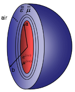
Figure 1: [Color online] Illustration of the cloaking shell covering the object to be concealed. We consider the spherical cloak in free space with the inner radius $k_{0}a=\pi$ and outer radius $k_{0}b=2\pi$. The core material is glass ($\varepsilon^{(co)}=1.45^{2}$ and $\mu^{(co)}=1$). These quantities are used throughout the whole paper. The material parameters $\overline{\overline{\varepsilon}}$ and $\overline{\overline{\mu}}$ are determined by applying the proposed transformation-free method to an arbitrary cloaking generating function. The cloaking shell is equally divided into $N$ layers (each layer is homogeneous and anisotropic), and the scattering theory in [36] is used to compute the far-field diagrams.

We will consider some typical generating functions (for transverse dielectric permittivities) which exhibit different types of profiles. The simplest generating functions are constant, linear, and quadratic ones. Which of them provides the best cloaking performance?

Constant generating function produces the dielectric permittivities of the Pendry’s classic spherical cloak as it has been demonstrated in the previous section. Linear generating function can be generally written as $g(r)=r-p$, where $p$ is a constant parameter. In this case transverse and radial dielectric permittivities become

$$\varepsilon_{t}(r)=\frac{2b(r-p)}{(b-a)(b+a-2p)},$$ (90)

$$\varepsilon_{r}=\frac{b(r-a)^{2}(r+a-2p)^{2}}{2r^{2}(r-p)(b-a)(b+a-2p)}.$$ (91)

Parameter $p$ can take any value except $(a+b)/2$. It controls the slope of the transverse permittivity function. If $p<(a+b)/2$, $\varepsilon_{t}(r)$ linearly increases, and otherwise it monotonically decreases.

Quadratic generating function has the general form $g(r)=(r-p)(r-d)+s$, where $p$, $d$, and $s$ are tunable parameters. The expressions for the permittivities in quadratic case can be deduced to

$$\varepsilon_{t}(r)=\frac{b[(r-p)(r-d)+s]}{P(b)},$$ (92)

$$\varepsilon_{r}=\frac{bP^{2}(r)}{r^{2}[(r-p)(r-d)+s]P(b)},$$ (93)

where

$$P(r)=\frac{r^{3}-a^{3}}{3}-(p+d)\frac{r^{2}-a^{2}}{2}+(pd+s)(r-a).$$ (94)

Quadratic transverse permittivity is a parabola in graphical presentation. The parabola can have a minimum (i.e., $s>s_{0}$) or maximum (i.e., $s<s_{0}$), where $s_{0}=-(b^{2}+ab+a^{2})/3+(p+d)(a+b)/2-pd$.

Using these generating functions, some typical situations depicted in Fig. 2 are presented. Profile 5 demonstrates the permittivities for the constant generating function $g(r)=1$ corresponding to Pendry’s cloak. Linear generating functions are presented in Profile 4 ($g(r)=r-a$) and Profile 6 ($g(r)=r-b$). The other profiles are produced using quadratic generating functions.

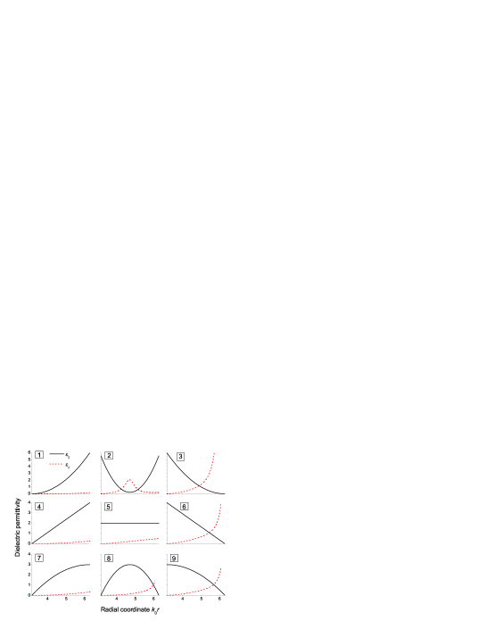
Figure 2: [Color online] Transverse $\varepsilon_{t}$ and radial $\varepsilon_{r}$ dielectric permittivities corresponding to different profiles of generating function. Profiles 1–9 are described as follows: (1) quadratic generating function with $p=0$, $d=b$, $s=b^{2}/4$; (2) quadratic generating function with $p=a$, $d=b$, $s=(b-a)^{2}/4+0.1$; (3) quadratic generating function with $p=a$, $d=2b-a$, $s=(b-a)^{2}$; (4) linear generating function with $p=a$; (5) constant generating function; (6) linear generating function with $p=b$; (7) quadratic generating function with $p=a$, $d=2b-a$, $s=0$; (8) quadratic generating function with $p=a$, $d=b$, $s=0$; (9) quadratic generating function with $p=0$, $d=b$, $s=0$.

The performances of different cloaks can be compared in terms of their scattering cross-sections. The best cloaking design possesses the lowest cross-section because of the reduced interaction of the electromagnetic wave with the spherical particle. The inhomogeneous anisotropic spherical cloaking shell is divided into $N$ homogeneous anisotropic spherical layers. An experimental realization of this multilayer cloak can be the sputtering onto the spherical core. Throughout the whole paper we use $N=30$.

In Fig. 3 the total cross-sections resulting from different generating functions are shown. Some profiles are approximately equivalent, for example, 1, 2 and 3, or 4 and 6, or 7 and 9. Profiles 1–3 are characterized by concave-up transverse dielectric permittivity $\varepsilon^{\prime\prime}_{t}>0$. According to Fig. 3 they give rise to the worst results. The flat-curvature profiles 4–6 characterized by $\varepsilon^{\prime\prime}_{t}=0$ are much better. Pendry’s cloak (number 5) stands out against the other zero-curvature profiles. However, the most effective cloak design is the case of concave-down transverse permittivity $\varepsilon^{\prime\prime}_{t}<0$. Profiles 7, 8, and 9 are better than profiles 4, 5, and 6, respectively, by approximately 4.8 dB. The quadratic cloak with concave-down transverse permittivity (bell-shaped cloak) is shown to be the best candidate.

The maximum of $\varepsilon_{t}$ in profile 8 is in the middle position of the cloaking shell. Shifting the maximum of such a bell shape towards the limit at the outer boundary (i.e., profile 7) or inner boundary (i.e., profile 9), the cloaking performance is monotonically degraded as shown in Fig. 3. If parameter $s$ is extremely huge in quadratic generating function ($s\rightarrow\infty$), the cloak permittivities coincide with those of Pendry’s cloak. Thus, the increase of $s$ improves the cloak 2 and deteriorates the cloak 8.

Figure 3: Total cross-sections for profiles of permittivities shown in Fig. 2. The number of discrete layers forming the cloak equals $N=30$.

4 The General Class of Bell-Shaped Cloaks

From the previous section it is concluded that the bell-shaped profile of the transverse dielectric permittivity leads to the optimal non-ideal cloaking performance. In the present section we will consider the general class of bell-shaped cloaks and choose the best type.

Apart from the quadratic cloak, another three simple bell-shaped profiles will be considered: Gaussian, Lorentzian, and Sech. All of them have a single parameter $T$, which sets the width of the profile. We take the maxima of such transverse permittivities in the middle of the cloaking shell region (at the point $(a+b)/2$) to compare with quadratic cloak.

Gaussian cloak has the generating function $g(r)=\exp[-(r-(a+b)/2)^{2}/(4T^{2})]$. The permittivity functions are

$$\varepsilon_{t} = \frac{b}{2\sqrt{\pi}T{\rm Erf}[(b-a)/(4T)]}{\rm e}^{-\frac{(r-(a+b)/2)^{2}}{4T^{2}}}$$

$$\varepsilon_{r} = \frac{\sqrt{\pi}Tb({\rm Erf}[(b+a-2r)/(4T)]-{\rm Erf}[(b-a)/(4T)])^{2}}{2r^{2}{\rm Erf}[(b-a)/(4T)]}{\rm e}^{\frac{(r-(a+b)/2)^{2}}{4T^{2}}}.$$ (95)

The generating function of the Lorentzian cloak is $g(r)=1/[1+(r-(a+b)/2)^{2}/T^{2}]$. The transverse and radial permittivities for this cloak are of the form

$$\varepsilon_{t} = \frac{b}{2T[1+(r-(a+b)/2)^{2}/T^{2}]\arctan[(b-a)/(2T)]}$$

$$\varepsilon_{r} = \frac{Tb(\arctan[(b+a-2r)/(2T)]-\arctan[(b-a)/(2T)])^{2}}{2r^{2}\arctan[(b-a)/(2T)]}\times$$ (96)

$$\left(1+\frac{(r-(a+b)/2)^{2}}{T^{2}}\right).$$

Sech cloak generating function depends on the radial coordinate as $g(r)={\rm sech}^{2}[(r-(a+b)/2)/T]$. The permittivities are as follows

$$\varepsilon_{t} = \frac{b{\rm sech}^{2}[(r-(a+b)/2)/T]}{2T\tanh[(b-a)/(2T)]}$$

$$\varepsilon_{r} = \frac{Tb(\tanh[(2r-b-a)/(2T)]-\tanh[(b-a)/(2T)])^{2}}{2r^{2}{\rm sech}^{2}[(r-(a+b)/2)/T]\tanh[(b-a)/(2T)]}.$$ (97)

We choose equal 3 dB bandwidths for various transverse permittivity profiles to compare different cloaks. Parameters $T$ which are tuned to provide identical 3 dB bandwidth for each cloak are given in the caption of Fig. 4. In this figure we show the total cross-sections of quadratic, Gaussian, Lorentzian, and Sech cloaks. Profiles of Gaussian, Lorentzian, and Sech cloaks are very close, resulting in similar scattering cross-sections. The influence of the permittivity functions on the cloak performance is difficult to tell among these three cloaks. However, it is shown that quadratic cloak in Fig. 4 provides better invisibility when its transverse permittivity vanishes at the inner and outer boundaries of the cloaking shell.

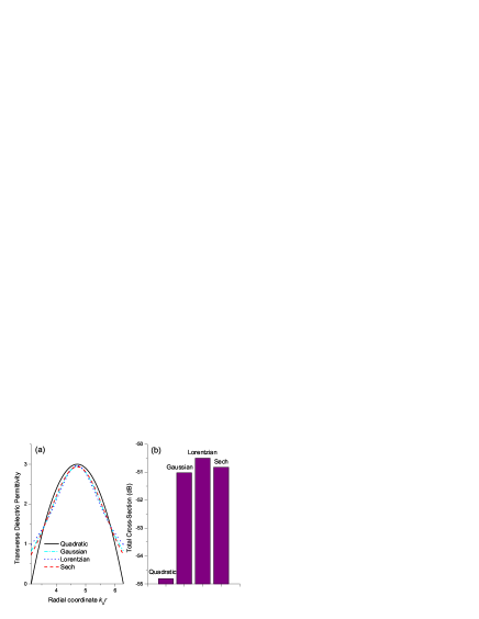
Figure 4: [Color online] (a) Profiles of transverse dielectric permittivity for quadratic (profile No. 8 in Fig. 2), Gaussian, Lorentzian, and Sech cloaks and (b) total cross-sections of these cloaks. Parameter $T$ equals $(b-a)/4\sqrt{2\ln 2}$ for Gaussian, $(b-a)/(2\sqrt{2})$ for Lorentzian, and $(b-a)/(2\sqrt{2}\ln(\sqrt{2}+1))$ for Sech cloak. The number of discrete layers forming the cloak equals $N=30$.

Since the shapes of the Gaussian, Lorentzian, and Sech cloaks are similar, we can just select one of them, (e.g., Gaussian) to investigate the significance of the profile, which can be varied by the parameter $T$. The results are demonstrated in Fig. 5. The total cross-section has a minimum, which does not provide better cloaking than quadratic one though. The cross-section minimization is achieved approximately at $T=0.3a$. This profile is shown in Fig. 5(a) along with profiles for other $T$ parameters. According to this figure the minimization profile has the 3 dB bandwidth equal $(b-a)/2$. Such a profile is neither too narrow nor too wide because narrow profiles ($T\rightarrow 0$) need extremely high discretization and wide profiles ($T\rightarrow\infty$) tend to the limit of Pendry’s cloak as shown in Fig. 5(b).

Thus the bell-shaped quadratic cloak is preferred for non-ideal cloak design, which has the lowest cross-section among all bell-shaped cloaks considered in this section. In the following section we will show how the quadratic cloak results can be improved.

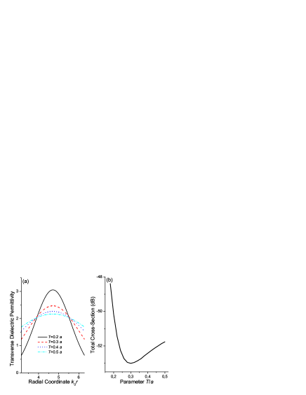
Figure 5: [Color online] (a) Profiles of transverse dielectric permittivity for Gaussian cloaks with different parameters $T$ and (b) total cross-sections versus parameter $T$. The number of discrete layers forming the cloak equals $N=30$.

5 Improved Quadratic Cloaks

Quadratic cloak is characterized by very simple profile of the transverse dielectric permittivity. Also, the quadratic cloak has the scattering almost 5 dB lower than that of classic spherical one. Our aim of this section is to find a way of creating the high-performance cloaks based on the transformation-free design method and bell-shaped quadratic cloak. The high-performance cloak should be similar to the quadratic one. Transverse permittivity should have a maximum and vanish at the inner and outer radii of the shell: $\varepsilon_{t}(a)=\varepsilon_{t}(b)=0$. These properties can be satisfied for general generating function of the form

$$g(r)=(r-a)(r-b)g_{1}(r).$$ (98)

By choosing function $g_{1}(r)$, we can set the permittivity profile of the cloak. The function $g_{1}(r)$ can take arbitrary values at the cloak edges $r=a$ and $r=b$, though it should provide the maximum of the transverse permittivity. At first we will consider the maximum at the center of the cloak $r=(a+b)/2$, and then the effect of the non-central maximum position will be studied. For instance function $g_{1}(r)$ can be selected with Gaussian profile. Then the cloak can be called Gaussian-quadratic one. However, such a design is worse than the simple quadratic shape. To provide the better design we will focus the quadratic dependence using the $g_{1}(r)$ function

$$g_{1}(r)=((r-p)(r-d)+(d-p)^{2}/4+s)^{n}.$$ (99)

When $n=0$, it is just the bell-shaped quadratic cloak discussed before. The permittivities at $n>0$ are suppressed due to lengthy expressions.

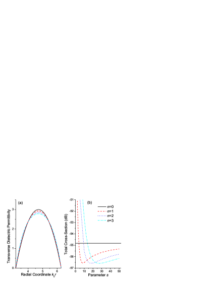
Figure 6: [Color online] (a) Profiles of transverse permittivity for power quadratic cloaks and (b) total cross-sections of these cloaks versus parameter $s$. Parameters: $p=a$, $d=b$, $N=30$. In (b), only $s>0$ is considered for cloaking purposes because the total cross-sections corresponding to $s<0$ are significantly larger.

In the generating function set by Eqs. (98) and (99) we can vary the power term $n$ (the curvature of the transverse permittivity profile at peak), parameters $s$ (the deviation from the quadratic cloak) and $d$ (the deviation of the permittivity peak from the center of the cloaking region). At $n=0$ the generating function is independent on $s$ and $d$ so the total cross-section is the straight line in Fig. 6 (the solid line), where other positive values of $n$ are shown as well. The minima of the cross-sections (the best cloaking performance) occurs to the parameter $s$ approximately at $s_{min}\approx 9n$, i.e., linear to the power $n$. At larger parameter $s$, the curves tend to the cross-section of the quadratic cloak. At small and negative $s$, the shape of the transverse permittivity contains the minimum and a couple of maxima, therefore the total cross-section is substantially increased. In Fig. 6(b), the cloaking performance is obviously improved compared with the quadratic cloak. Let us further study the effect of the peak position of the profile, which is controlled by the parameter $d$.

The case $d=b$ describes that the position of the permittivity maximum is in the center of the cloaking shell region. If $d<b$ ($d>b$), the maximum is shifted towards the outer (inner) radius of the cloaking shell. Fig. 7 shows that the central position of the permittivity maximum is not the optimal choice. The minimization of the cross-section is achieved for $d\approx 0.84b$. Such a non-central position is expected to result from the spherically curvilinear geometry of the cloak.

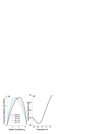
Figure 7: [Color online] (a) Profiles of transverse dielectric permittivity for power quadratic cloaks and (b) total cross-sections of these cloaks vs. parameter $d$. Parameters: $p=a$, $n=2$, $s=18$, $N=30$.

Compared with the quadratic cloak, the improvement of the performance of power quadratic cloak is considerable: the total cross-section is further decreased from $-54.84$ dB to $-57.52$ dB. The improvement is caused by the shape of the profile. The profile should be parabolic-like with a slightly deformed shape.

It is also important to consider the differential cross-sections which provides the scattering intensity at an arbitrary angle. In Fig. 8 we show the differential cross-sections for some typical cloaking designs designed by the transformation-free method and considered in a non-ideal situation. The common feature of the cloaks is the reduced backscattering. It is seen that the classic spherical cloak is the most visible one. The quadratic cloak (blue dotted line) can provide much lower scattering over almost all angles compared with Pendry’s and Gaussian’s bell-shaped cloak. The power quadratic cloak is able to further bring down the scattering of the quadratic cloak near the forward direction.

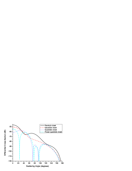
Figure 8: [Color online] Differential cross-sections of the cloaks derived by the proposed transformation-free method. The cloak parameters of each given design have been selected to provide the best performance respectively. Parameters: $T=0.3a$ for Gaussian cloak; $s=18$, $n=2$, $p=a$, and $d=0.84b$ for power quadratic cloak; $N=30$.

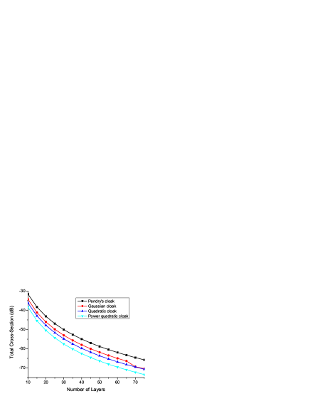
Figure 9: [Color online] Total cross-sections of different cloak designs versus the number of spherical layers $N$. Parameters of the cloaks are the same as those in Fig. 8.

However, one may question that our non-ideal situation may approach to the ideal case when the discretization is high (i.e., $N$ is much larger than 30). If so, each cloak derived from our proposed reversed algorithm should be more and more identical to each other. Theoretically, it is true provided that $N\rightarrow\infty$, while the influence of the disretization number $N$ on the optimization result is still of significant importance in practice. We calculate the total cross-sections for different numbers of spherical layers in Fig. 9. In general, we observe the conservation of our conclusions on the optimization for $N=30$, except for that the performance of the Gaussian cloak matches with that of the quadratic cloak at $N=70$. When $N$ is small, the dependence of scattering reduction on the value of $N$ is nonlinear. For great number of layers $N$ the curves become mostly linear as shown in Fig. 9.

6 Conclusion

It has been found that the bell-shaped cloaks provide the smallest interaction of the cloaking shell with the electromagnetic radiation under the non-ideal situation (i.e., the cloaking shell is discretized into $N$ layers). Among the bell-shaped cloaks, we have compared quadratic, Gaussian, Lorentzian, and Sech cloaks. The last three are very similar in profile shape and dependence of controlling parameters. We have concluded that the best performance is achieved when the bell-shaped transverse permittivity profiles which vanish at the inner and outer radii of the cloaking shell. The simplest design of such a type is the quadratic cloak. Improved invisibility performance can be provided by the power quadratic cloak with the maximum of the permittivity profile slightly shifted towards the outer boundary. The decrease of cloak’s overall scattering is about 7.5 dB compared with the classical Pendry’s design, and the improvement is steady even when the discretization $N$ is quite high.

References

References

- [1] Pendry J B, Schurig D and Smith D R 2006 Science 312 1780
- [2] Leonhardt U Science 2006 312 1777
- [3] Schurig D, Mock J J, Justice B J, Cummer S A, Pendry J B, Starr A F and Smith D R 2006 Science 314 977
- [4] Liu R, Ji C, Mock J J, Chin J Y, Cui T J and Smith D R 2009 Science 323 366-369
- [5] Leonhardt U 2006 New J. Phys. 8 118
- [6] Miller D A B 2006 Opt. Express 14 12457
- [7] Schurig D, Pendry J B and Smith D R 2006 Opt. Express 14 9794
- [8] Nicorovici N A P, Milton G W, McPhedran R C and Botten L C 2007 Opt. Express 15 6314
- [9] Liang Z X, Yao P J, Sun X W and Jiang X Y 2008 Appl. Phys. Lett. 92 131118
- [10] Zhao Y, Argyropoulos C and Hao Y 2008 Opt. Express 16 6717
- [11] Cai W S, Chettiar U K, Kildishev A V and Shalaev V M 2007 Nat. Photonics 1 224
- [12] Cai W S, Chettiar U K, Kildishev A V and Shalaev V M 2008 Opt. Express 16 5444
- [13] Vanbesien O, Fabre N, Melique X and Lippens D 2008 Appl. Opt. 47 1358
- [14] Xiao D and Johnson H T 2008 Opt. Lett. 33 860
- [15] Jenkins A 2008 Nat. Photonics 2 270
- [16] Valentine J, Li J, Zentgraf T, Bartal G and Zhang X 2009 Nat. Mater. doi:10.1038/nmat2461
- [17] Milton G W, Briane M and Willis J R 2006 New J. Phys. 8 248
- [18] Farhat M, Guenneau S, Enoch S and Movchan A B 2009 Phys. Rev. B 79 033102
- [19] Zhang S, Genov D A, Sun C and Zhang X 2008 Phys. Rev. Lett. 100 123002
- [20] Greenleaf A, Kurylev Y, Lassas M and Uhlmann G 2008 Phys. Rev. Lett. 101 220404
- [21] Chen H and Chan C T 2007 Appl. Phys. Lett. 91 183518
- [22] Cummer S A and Schurig D 2007 New J. Phys. 9 45
- [23] Cai L W and Sanchez-Dehesa J 2007 New J. Phys. 9 450
- [24] Cummer S A, Popa B I, Schurig D, Smith D R, Pendry J, Rahm M and Starr A 2008 Phys. Rev. Lett. 100 024301
- [25] Greenleaf A, Lassas M and Uhlmann G 2003 Physiol. Meas. 24 413
- [26] Chen H, Wu B I, Zhang B and Kong J A 2007 Phys. Rev. Lett. 99 063903
- [27] Zhang B, Chen H, Wu B I and Kong J A 2008 Phys. Rev. Lett. 100 063904
- [28] Gao L, Fung T H, Yu K W and Qiu C W 2008 Phys. Rev. E 78 046609
- [29] Ni Y X, Gao L and Qiu C W 2009 Preprint 0905.1503 [physics.optics]
- [30] Alu A and Engheta N 2007 Opt. Express 15 3318
- [31] Kwon D and Werner D H 2008 Appl. Phys. Lett. 92 013505
- [32] Jiang W X, Cui T J, Yu G X, Lin X Q, Cheng Q and Chin J Y 2008 J. Phys. D: Appl. Phys. 41 085504
- [33] Nicolet A, Zolla F and Guenneau S 2008 Opt. Lett. 33 1584
- [34] Qiu C W, Li L W, Yeo T S and Zouhdi S 2007 Phys. Rev. E 75 026609
- [35] Qiu C W, Hu L, Xu X and Feng Y 2009 Phys. Rev. E 79 047602
- [36] Qiu C W, Novitsky A, Ma H and Qu S 2009 Preprint 0905.1703 [physics.optics]