Hysteresis effects and diagnostics of the shock formation in low angular momentum axisymmetric accretion in the Kerr metric

Abstract

The secular evolution of the purely general relativistic low angular momentum accretion flow around a spinning black hole is shown to exhibit hysteresis effects. This confirms that a stationary shock is an integral part of such an accretion disc in the Kerr metric. The equations describing the space gradient of the dynamical flow velocity of the accreting matter have been shown to be equivalent to a first order autonomous dynamical systems. Fixed point analysis ensures that such flow must be multi-transonic for certain astrophysically relevant initial boundary conditions. Contrary to the existing consensus in the literature, the critical points and the sonic points are proved not to be isomorphic in general, they can form in a completely different length scales. Physically acceptable global transonic solutions must produce odd number of critical points. Homoclinic orbits for the flow flow possessing multiple critical points select the critical point with the higher entropy accretion rate, confirming that the entropy accretion rate is the degeneracy removing agent in the system. However, heteroclinic orbits are also observed for some special situation, where both the saddle type critical points of the flow configuration possesses identical entropy accretion rate. Topologies with heteroclinic orbits are thus the only allowed non removable degenerate solutions for accretion flow with multiple critical points, and are shown to be structurally unstable. Depending on suitable initial boundary conditions, a homoclinic trajectory can be combined with a standard non homoclinic orbit through an energy preserving Rankine-Hugoniot type of stationary shock, and multi-critical accretion flow then becomes truly multi-transonic. An effective Lyapunov index has been proposed to analytically confirm why certain class of transonic flow can not accommodate shock solutions even if it produces multiple critical points.

1 Whither shocked accretion disc?

For accretion of matter onto astrophysical black holes, the local radial Mach number $M$ of the accreting fluid can be defined as the ratio of the radial component of the local dynamical flow velocity to that of the propagation of the acoustic perturbation embedded inside the accreting matter. The flow will be locally subsonic or supersonic according to $M<1$ or $>1$. The flow is transonic if at any moment it crosses the $M=1$ hypersurface. This happens when a subsonic to supersonic or supersonic to subsonic transition takes place either continuously or discontinuously. The point(s) where such crossing takes place continuously is (are) called sonic point(s), and where such crossing takes place discontinuously are called shocks or discontinuities. The particular value of the radial distance $r$ for which $M=1$, is referred as the transonic point or the sonic point, and will be denoted by $r_{s}$ hereafter. For $r<r_{s}$, infalling matter becomes supersonic. Any acoustic perturbation created in such a region is destined to be dragged toward the black hole, and can not escape to the domain $r>r_{s}$. In other words, any co-moving observer from $r<r_{s}$ region can not communicate with any observer (co-moving or stationary) located in the sub-domain $r>r_{s}$ by sending any signal which travels with velocity $v_{\rm signal}{\leq}c_{s}$, where $c_{s}$ is defined as the velocity of propagation of the acoustic perturbation (the sound speed) embedded in the moving fluid. Hence the hypersurface through $r_{s}$ is generated by the acoustic null geodesics, i.e., by the phonon trajectories, and is actually an acoustic horizon for stationary configuration, which is produced when accreting fluid makes a transition from subsonic ($M<1$) to the supersonic ($M>1$) state. At a distance far away from the black hole, accreting material almost always remains subsonic (except possibly for the supersonic stellar wind fed accretion) since it possesses negligible dynamical flow velocity. On the other hand, the flow velocity will approach the velocity of light $c$ while crossing the event horizon, while the maximum possible value of sound speed, even for the steepest possible equation of state, would be $c/\sqrt{3}$, resulting $M>1$ close to the event horizon. In order to satisfy such inner boundary condition imposed by the event horizon, accretion onto black holes exhibit transonic properties in general, see, e.g., Pringle (1981); Chakrabarti (1990); Kato, Fukue & Mineshige (1998); Frank et al. (2002) for further details.

It will be shown in the subsequent sections that the physical transonic accretion solutions can formally be realized as critical solution on the phase portrait (spanned by dynamical flow/Mach number and the radial distance) of the black hole accretion. It will also be discussed, in great details, that usually a critical point is not identical with a sonic point. For sub-Keplerian angular momentum distribution of matter, frequently it happens that the critical features are exhibited more than once in the phase portrait of a stationary solutions describing an axisymmetric black hole accretion. For such situations, the number of critical points, unlike spherical accretion, may exceed one. A large pool of literature, dealing with the theory of the black hole accretion disc, studied various properties of such flows with multiple critical points (Liang & Thompson, 1980; Abramowicz & Zurek, 1981; Muchotrzeb & Paczyński, 1982; Muchotrzeb, 1983; Fukue, 1983, 1987, 2004, 2004a; Lu, 1985, 1986; Muchotrzeb-Czerny, 1986; Abramowicz & Kato, 1989; Abramowicz & Chakrabarti, 1990; Chakrabarti, 1990; Kafatos & Yang, 1994; Yang & Kafatos, 1995; Pariev, 1996; Peitz & Appl, 1997; Caditz & Tsuruta, 1998; Das, 2002; Barai et al., 2004; Abraham et al., 2006; Das, 2007).

For realistic astrophysical systems, such sub-Keplerian weakly rotating flows are exhibited in various physical situations, such as detached binary systems fed by accretion from OB stellar winds (Illarionov & Sunyaev (1975); Liang & Nolan (1980)), semi-detached low-mass non-magnetic binaries ( Bisikalo et al. (1998)), and super-massive black holes fed by accretion from slowly rotating central stellar clusters (Illarionov (1988); Ho (1999) and references therein). Even for a standard Keplerian accretion disc, turbulence may produce such low angular momentum flow (see, e.g., Igumenshchev & Abramowicz (1999), and references therein).

In supersonic astrophysical flows, perturbation of various kinds may produce discontinuities. Such discontinuities are said to take place over one or more surfaces when any dynamical and/or thermodynamic quantity changes discontinuously as such surfaces are crossed. The corresponding surfaces are called the surfaces of discontinuity. Certain boundary conditions are to be satisfied across such surfaces, and according to those conditions, surfaces of discontinuities are classified into various categories, the most important being the shock waves or shocks. Such shock waves are quite often generated in various kinds of supersonic astrophysical flows having intrinsic angular momentum, resulting the final state of the flow to be subsonic. This is because the repulsive centrifugal potential barrier experienced by such flows is sufficiently strong to brake the infalling motion and a stationary solution could be introduced only through a shock. Rotating, transonic astrophysical fluid flows are thus believed to be ‘prone’ to the shock formation phenomena.

The non-linear equations describing the steady, inviscid axisymmetric flow in the Kerr metric can be tailored to form a first order autonomous dynamical system. Physical transonic solution in such flows can be represented mathematically as critical solutions in the velocity (or Mach number) phase plane of the flow – they are associated with the critical points (alternatively known as the fixed points or the equilibrium points, see Jordan & Smith (1999) and Chicone (2006) for further details about the fixed point analysis techniques). To maintain the transonicity such critical points will perforce have to be saddle points, which will enable a solution to pass through themselves.

Before we proceed further, it is important to introduce a few nomenclatures we will be following in this work. When a configuration can have multiple critical points accessible to the accretion flow, we will mention it as ‘multi-critical’ accretion. Critical points for a non dissipative system can be of two types, either saddle or centre. A saddle type critical points allows an accretion flow to pass through it whereas a centre type critical point does not. Hence the concept of a ‘sonic point’ can only be associated with a saddle type critical point and not with a centre type one. No transonic solution can pass through a centre type critical point. We will demonstrate that a saddle type critical point usually has a sonic point associated with it. As a result, a multi-critical flow having three critical points, two saddle and one centre type, can only have two sonic points. A ‘multi-transonic’ flow, according to our definition, will be a particular subclass of multi-critical transonic accretion which can pass through two sonic points. This is possible, as we will see in subsequent sections, only if a shock forms. Otherwise, even if a flow has more than one saddle type critical points, transonic accretion passes only through a single sonic point. Such flows will in generally be termed as a ‘multi-ctritical mono-transonic’ flow in our work. On the contrary, when the number of the critical point itself is one, and that critical point is of saddle type so that a sonic point is also associated with the flow, we will call it a ‘mono-critical mono-transonic’ flow. We will see in the subsequent sections that among the several phases of the transonic accretion flow, a true multi-transonic flow forms only for a shocked accretion, otherwise all accretion flows are mono-transonic: either of the multi-critical mono-transonic category or of mono-critical mono-transonic category. All these issues will further be elaborated with greater detail in subsequent sections.

The true multi-transonicity in the Kerr geometry implies the existence of three critical points and a standing shock, and under the fundamental physical requirement of accretion being a process whereby a flow solution should connect infinity to the event horizon of the black hole, the three critical points should be such that there would be two saddle points flanking a centre type point between themselves. Originating at a large distance, subsonic accretion encounters the outermost saddle type sonic point and becomes supersonic. Subjected to the appropriate perturbative environment, such supersonic flow encounters a shock and becomes subsonic again. Such subsonic matter has to pass through another saddle type sonic point to meet the aforesaid inner boundary condition. For accretion onto black hole, presence of at least two saddle type sonic points are thus a necessary (but not sufficient) condition for the shock formation. Multi-transonicity, thus, plays a crucial role in studying the physics of shock formation and related phenomena in connection to the black hole accretion processes.

One also expects that a shock formation in black-hole accretion discs might be a general phenomenon because shock waves in rotating astrophysical flows potentially provide an important and efficient mechanism for conversion of a significant amount of the gravitational energy into radiation by randomizing the directed infall motion of the accreting fluid. Hence, the shocks play an important role in governing the overall dynamical and radiative processes taking place in astrophysical fluids and plasma accreting onto black holes.

The hot and dense post shock flow is considered to be a powerful diagnostic tool in understanding various astrophysical phenomena like the spectral properties of the galactic black hole candidates (Chakrabarti & Titarchuk, 1995) and that of the supermassive black hole at our Galactic centre (Moscibrodzka, Das & Czerny, 2006), the formation and dynamics of accretion powered galactic and extra-galactic outflows (Das & Chakrabarti, 1999; Chattopadhyay & Das, 2007; Das & Chattopadhyay, 2007), shock induced nucleosynthesis in the black hole accretion disc and the metalicity of the intergalactic matter ((Mukhopadhyay, 1999) and references therein), and the origin of the quasi-periodic oscillation in galactic sources ((Sponholz & Molteni, 1994; Das, Rao & Vadawale, 2003; Okuda et al., 2004, 2007) and references therein).

The study of steady, standing, stationary shock waves produced in black hole accretion and related phenomena thus acquired an important status in recent years( (Fukue, 1983, 1987, 2004, 2004a; Kato et al., 198yy8; Chakrabarti, 1989; Kafatos & Yang, 1994; Yang & Kafatos, 1995; Caditz & Tsuruta, 1998; Fukumura & Tsuruta, 2004; Takahashi et al., 1992; Das, 2002; Lu et al., 1997; Lu & Gu, 2004; Nakayama & Fukue, 1989; Nagakura & Yamada, 2008; Nakayama, 1996; Nagakura & Yamada, 2009; Tóth, Keppens, & Botchev, 1998)). However, since for the same set of initial boundary conditions describing the multi-transonic accretion, there exist flow profiles which may or may not accommodate shock solutions, the very existence of accretion flow with shock is still a matter of debate to the astrophysical community involved in the study of the theory of black hole accretion disc.

This present treatment confirms, using a much broader and more comprehensive procedure in its scope and objectives than those reported previously in the literature, that the shock is an integral part of the black hole axisymmetric accretion in its most generic form, i.e., for the general relativistic accretion disc in the Kerr metric. In the present paper we study the sequence of the stationary axisymmetric solutions characterized by the angular momentum paying attention to the changes of the flow topology in the extended velocity phase space diagram. By the phrase ‘extended velocity phase diagram’, here we mean the two dimensional graphical representation where the radial Mach number has been plotted along the ordinate and the radial distance has been plotted along the abscissa. The radial Mach number is the ratio of the radial velocity measured on the equatorial plane of the accretion disc, and the height averaged polytropic sound speed defined on the equatorial plane of the disc. The radial distance has been measured from the black hole along the equatorial plane, and is scaled in the units of $GM_{BH}/c^{2}$, where $G$ is the Universal gravitational constant and $M_{BH}$ is the mass of the black hole considered, $G$ and $c$ have been scaled to be unity in the system of geometrical unit. We discuss in detail the critical solution which divides the family of compact transonic flows (solutions with sonic point at the innermost critical point) from extended transonic flows (solutions with sonic point at the outermost critical point). We argue that the existence of this critical solution is likely to lead to a hysteresis effect when the system chooses the solution with, or without a shock, depending on the flow history. In addition, we have proposed a Lyapunov like treatment, to show that the likelihood of the event that a shock will form or not, clearly depends on the value of such effective Lyapunov index.

The plan of the paper is as follows:

In the next section, we will describe the overall flow configuration, and the corresponding governing equations will be derived, solution of which, along with a detailed discussion of the transonic properties arising out of such solutions, will be provided in the section 3 Section 4 and 5 will elaborate the multi-transonic behaviour of such flow. In section 6 we will describe certain ‘hysteresis effects’ corresponding to the secular evolution of the flow. Section 7 will illustrate the details of an Lyapunov like treatment for the state transition in transonic accretion solution to establish what prompts a multi-transonic accretion to (or not to) contain a standing shock solution. Finally we conclude in the section 8.

2 Dressing up the disc

2.1 Spacetime geometry and the stress energy tensor

To provide a generic description of axisymmetric fluid flow in strong gravity, one needs to solve the equations of motion for the fluid and the Einstein equations. As of our present (limited) understanding about the detail physics of the black hole accretion flow is concerned, this seems to be an enormously difficult, if not impossible, task to accomplish. The problem may be made relatively tractable by assuming the accretion to be non-self gravitating so that the fluid dynamics may be dealt in a metric without back-reactions. The most general form of the energy momentum tensor for such non self gravitating compressible hydromagnetic astrophysical fluid (with a frozen in magnetic field) vulnerable to the shear, bulk viscosity and generalized energy exchange, may be expressed as (Novikov & Thorne, 1973):

$${\large\sf T}^{{\mu}{\nu}}={\large\sf T}^{{\mu}{\nu}}_{\sf M}+{\large\sf T}^{{\mu}{\nu}}_{\large\sf B}$$ (1)

where ${\large\sf T}^{{\mu}{\nu}}_{\sf M}$ and ${\large\sf T}^{{\mu}{\nu}}_{\large\sf B}$ are the fluid (matter) part and the Maxwellian (electromagnetic) part of the energy momentum tensor. ${\large\sf T}^{{\mu}{\nu}}_{\sf M}$ and ${\large\sf T}^{{\mu}{\nu}}_{\large\sf B}$ may be expressed as:

$${\large\sf T}^{{\mu}{\nu}}_{\sf M}={\rho}v^{\mu}v^{\nu}+\left(p-\varsigma{\theta}\right)h^{\mu\nu}-2\eta{\sigma}^{\mu\nu}+{\rm q}^{\mu}v^{\nu}+v^{\mu}{{\rm q}^{\nu}},~{}{\large\sf T}^{{\mu}{\nu}}_{\large\sf B}=\frac{1}{8\pi}\left({\rm B}^{2}v^{\mu}v^{\nu}+{\rm B}^{2}h^{\mu\nu}-2{\rm B}^{\mu}{\rm B}^{\nu}\right)$$ (2)

In the above expression, ${\rho}v^{\mu}v^{\nu}$ is the total mass energy density excluding the frozen-in magnetic field mass energy density as measured in the local rest frame of the baryons (local orthonormal frame, hereafter LRF, in which there is no net baryon flux in any direction). $ph^{\mu\nu}$ is the anisotropic pressure for incompressible gas (had it been the case that $\theta$ would be zero). $\varsigma$ and $\eta$ are the co-efficient of bulk viscosity and of dynamic viscosity, respectively. Hence $-\varsigma{\theta}h^{\mu\nu}$ and $-2{\eta}{\sigma^{\mu\nu}}$ are the bulk viscosity and the viscous shear stress, respectively. ${\rm q}^{\mu}v^{\nu}+v^{\mu}{{\rm q}^{\nu}}$ is the energy and momentum flux, respectively, in LRF of the baryons. In the expression for ${\large\sf T}^{{\mu}{\nu}}_{\large\sf B}$, ${\rm B}^{2}/8\pi$ in the first term represents the energy density, in the second term represents the magnetic pressure orthogonal to the magnetic field lines, and in third term magnetic tension along the field lines (all terms expressed in LRF), respectively.

Here, the electromagnetic field may be described by the field tensor ${\cal F}^{{\mu}{\nu}}$ and it’s dual ${\cal F}^{{\ast}{\mu}{\nu}}$ (obtained from ${\cal F}^{{\mu}{\nu}}$ using Levi-Civita totally antisymmetric tensor ${\epsilon}^{{\mu}{\nu}{\alpha}{\beta}}$) satisfying the Maxwell equations through the vanishing of the four-divergence of ${\cal F}^{{\ast}{\mu}{\nu}}$. A complete description of flow behaviour could thus be obtained by taking the co-variant derivative of ${\large\sf T}^{{\mu}{\nu}}$ and ${\rho}v^{\mu}$ to obtain the energy momentum conservation equations and the conservation of baryonic mass.

However, at this stage, the complete solution remains analytically untenable unless we are compelled to adopt a number of simplified approximations. Our work concentrates on the inviscid accretion of hydrodynamic fluid. Hence ${\large\sf T}^{{\mu}{\nu}}$ may be described by the standard form of the energy momentum (stress-energy) tensor of a perfect fluid:

$${\large\sf T}^{{\mu}{\nu}}=\left(\epsilon+p\right)v_{\mu}v_{\nu}+pg_{{\mu}{\nu}},~{}{\rm or,}~{}{\bf T}=\left(\epsilon+p\right){\bf v}{\otimes}{\bf v}+p{\bf g}$$ (3)

Our calculation will thus be focused on the stationary axisymmetric solution of the energy momentum and baryon number conservation equations

$${{\large\sf T}^{{\mu}{\nu}}}_{;\nu}=0;\;\;\;\;\;\left({\rho}{v^{\mu}}\right)_{;\mu}=0,$$ (4)

Specifying the metric to be stationary and axially symmetric, the two generators $\xi^{\mu}\equiv(\partial/\partial t)^{\mu}$ and $\phi^{\mu}\equiv(\partial/\partial\phi)^{\mu}$ of the temporal and axial isometry, respectively, are Killing vectors.

To describe the flow, it is advisable to use the Boyer-Lindquist co-ordinate Boyer & Lindquist (1967), and an azimuthally Lorentz boosted orthonormal tetrad basis co-rotating with the accreting fluid. At this stage we are not interested in non-axisymmetric disc structure, hence we neglect any gravo-magneto-viscous non-alignment between the flow angular momentum and the black hole spin angular momentum. We consider inviscid accretion and denote the constant specific flow angular momentum to be $\lambda$. Hence, while describing the accretion disc dynamics, the viscous transport of the angular momentum has not explicitly been taken into account. Viscosity, however, is quite a subtle issue in studying the disc accretion. Even thirty six years after the discovery of standard accretion disc theory (Shakura & Sunyaev, 1973; Novikov & Thorne, 1973), exact modeling of viscous transonic black-hole accretion, including proper heating and cooling mechanisms, is still quite an arduous task, even for a Newtonian flow, let alone for general relativistic accretion. Nevertheless, extremely large radial velocity close to the black hole implies $\tau_{inf}\ll\tau_{visc}$, where $\tau_{inf}$ and $\tau_{visc}$ are the infall and the viscous time scales, respectively. Large radial velocities even at larger distances are due to the fact that the angular momentum content of the accreting fluid is relatively low (Beloborodov & Illarionov, 1991; Igumenshchev & Beloborodov, 1997; Proga & Begelman, 2003). Hence, the assumption of inviscid flow is not unjustified from an astrophysical point of view. However, one of the most significant effects of the introduction of viscosity would be the reduction of the angular momentum. In our work, it has been observed that the location of the sonic points anti-correlates with $\lambda$, i.e. weakly rotating flow makes the dynamical velocity gradient steeper, which indicates that for viscous flow the sonic horizons will be pushed further out and the flow would become supersonic at a larger distance for the same set of other initial boundary conditions. Also we found how the shock location (and strength, and other related variables) get modified because of the variation of the flow angular momentum. Hence in our work, we practically have demonstrated the effect of viscosity as well.

We consider the flow to be ‘advective’, i.e. to possess considerable radial three-velocity. The above-mentioned advective velocity, which we hereafter denote by $u$ and consider it to be confined on the equatorial plane, is essentially the three-velocity component perpendicular to the set of hypersurfaces $\{\Sigma_{v}\}$ defined by $v^{2}={\rm const}$, where $v$ is the magnitude of the 3-velocity. Each $\Sigma_{v}$ is timelike since its normal $\eta_{\mu}\propto\partial_{\mu}v^{2}$ is spacelike and may be normalized as $\eta^{\mu}\eta_{\mu}=1$.

We then define the specific angular momentum $\lambda$ and the angular velocity $\Omega$ as

$$\lambda=-\frac{v_{\phi}}{v_{t}};\;\;\;\;\;\Omega=\frac{v^{\phi}}{v^{t}}=-\frac{g_{t\phi}+\lambda{g}_{tt}}{{g_{\phi{\phi}}+\lambda{g}_{t{\phi}}}}\,,$$ (5)

The metric on the equatorial plane is given by (Novikov & Thorne (1973))

$$ds^{2}=g_{{\mu}{\nu}}dx^{\mu}dx^{\nu}=-\frac{r^{2}{\Delta}}{A}dt^{2}+\frac{A}{r^{2}}\left(d\phi-\omega{dt}\right)^{2}+\frac{r^{2}}{\Delta}dr^{2}+dz^{2},$$ (6)

where $\Delta=r^{2}-2r+a^{2},~{}A=r^{4}+r^{2}a^{2}+2ra^{2}$, and $\omega=2ar/A$, $a$ being the Kerr parameter related to the black-hole spin. The normalization condition $v^{\mu}{v}_{\mu}=-1$, together with the expressions for $\lambda$ and $\Omega$ in (5), provides the relationship between the advective velocity $u$ and the temporal component of the four velocity

$$v_{t}=\left[\frac{Ar^{2}\Delta}{\left(1-u^{2}\right)\left\{A^{2}-4\lambda arA+\lambda^{2}r^{2}\left(4a^{2}-r^{2}\Delta\right)\right\}}\right]^{1/2}.$$ (7)

In order to solve (4), we need to specify a realistic equation of state. In this work, we concentrate on polytropic accretion, and some relevant details of the flow thermodynamics is presented in the next section.

It is to be noted here that the use of the polytropic equation of state in describing the thermodynamic properties of the accreting matter is quite common in the theory of relativistic black hole accretion. However, one also understands that the polytropic accretion is not the only choice to describe such accretion. Equations of state other than the adiabatic one, such as the isothermal equation  (Yang & Kafatos, 1995) or the two-temperature plasma  (Manmoto, 2000), have also been used to for this purpose.

2.2 The thermodynamics of the flow

The polytropic equation is taken to be of the following form

$$p=K{\rho}^{\gamma},$$ (8)

where the polytropic index $\gamma$ (equal to the ratio of the two specific heats $c_{p}$ and $c_{v}$) of the accreting material is assumed to be constant throughout the fluid. A more realistic model of the flow would perhaps require a variable polytropic index having a functional dependence on the radial distance, i.e. of the functional form $\gamma{\equiv}\gamma(r)$; see, e.g., (Ryu, Chattopadhyay & Choi, 2006) and references therein for further discussions. However, we have performed the calculations for a sufficiently large range of $\gamma$ and we believe that all astrophysically relevant polytropic indices are covered in our analysis.

The constant $K$ in (8) may be related to the specific entropy of the fluid, provided there is no entropy generation in the flow. If in addition to (8) the Clapeyron equation for an ideal gas holds

$$p=\frac{\kappa_{B}}{{\mu}m_{p}}{\rho}T\,,$$ (9)

where $T$ is the locally measured temperature, $\mu$ the mean molecular weight, $m_{H}{\sim}m_{p}$ the mass of the hydrogen atom, then the specific entropy, i.e. the entropy per particle, is given by  (Landau & Lifshitz, 1987):

$$\sigma=\frac{1}{\gamma-1}\log K+\frac{\gamma}{\gamma-1}+{\rm constant},$$ (10)

where the constant depends on the chemical composition of the accreting material. Equation (10) confirms that $K$ in (8) is a measure of the specific entropy of the accreting matter.

The specific enthalpy of the accreting matter can now be defined as

$$h=\frac{\left(p+\epsilon\right)}{\rho}\,,$$ (11)

where the energy density $\epsilon$ includes the rest-mass density and the internal energy and may be written as

$$\epsilon=\rho+\frac{p}{\gamma-1}\,.$$ (12)

The adiabatic speed of sound is defined by

$$c_{s}^{2}=\frac{{\partial}p}{{\partial}{\epsilon}}{\Bigg{|}}_{\rm constant~{}entropy}\,.$$ (13)

From (12) we obtain

$$\frac{\partial{\rho}}{\partial{\epsilon}}=\left(\frac{\gamma-1-c_{s}^{2}}{\gamma-1}\right).$$ (14)

Combination of (13) and (8) gives

$$c_{s}^{2}=K{\rho}^{\gamma-1}{\gamma}\frac{\partial{\rho}}{\partial{\epsilon}}\,,$$ (15)

Using the above relations, one obtains the expression for the specific enthalpy

$$h=\frac{\gamma-1}{\gamma-1-c_{s}^{2}}\,.$$ (16)

The rest-mass density $\rho$, the pressure $p$, the temperature $T$ of the flow and the energy density $\epsilon$ may be expressed in terms of the speed of sound $c_{s}$ as

$$\rho=K^{-\frac{1}{\gamma-1}}\left(\frac{\gamma-1}{\gamma}\right)^{\frac{1}{\gamma-1}}\left(\frac{c_{s}^{2}}{\gamma-1-c_{s}^{2}}\right)^{\frac{1}{\gamma-1}},$$ (17)

$$p=K^{-\frac{1}{\gamma-1}}\left(\frac{\gamma-1}{\gamma}\right)^{\frac{\gamma}{\gamma-1}}\left(\frac{c_{s}^{2}}{\gamma-1-c_{s}^{2}}\right)^{\frac{\gamma}{\gamma-1}},$$ (18)

$$T=\frac{\kappa_{B}}{{\mu}m_{p}}\left(\frac{\gamma-1}{\gamma}\right)\left(\frac{c_{s}^{2}}{\gamma-1-c_{s}^{2}}\right),$$ (19)

$$\epsilon=K^{-\frac{1}{\gamma-1}}\left(\frac{\gamma-1}{\gamma}\right)^{\frac{1}{\gamma-1}}\left(\frac{c_{s}^{2}}{\gamma-1-c_{s}^{2}}\right)^{\frac{1}{\gamma-1}}\left[1+\frac{1}{\gamma}\left(\frac{c_{s}^{2}}{\gamma-1-c_{s}^{2}}\right)\right].$$ (20)

We now need to define a specific geometrical structure of the disc, which has been done in the next section.

2.3 The disc geometry

We assume that the disc has a radius-dependent local thickness $H(r)$, and its central plane coincides with the equatorial plane of the black hole. It is a standard practice in accretion disc theory (Matsumoto et al. (1984); Paczyński (1987); Abramowicz et al. (1988); Chen & Taam (1993); Kafatos & Yang (1994); Artemova et al. (1996); Narayan, Kato & Honma (1997); Wiita (1998); Hawley & Krolik (2001); Armitage, Reynolds & Chiang (2001) and many others) to use the vertically averaged model in describing the black-hole accretion discs where the equations of motion apply to the equatorial plane of the black hole. We follow the same procedure here. The thermodynamic flow variables are averaged over the disc height, i.e., a thermodynamic quantity $y$ used in our model is vertically averaged over the disc height as

$$\bar{y}=\frac{\int^{H}(r)_{0}(ydh)}{\int^{H}(r)_{0}H(r)}.$$

We follow Abramowicz, Lanza & Pervival (1997) to derive an expression for the disc height $H(r)$ in our flow geometry since the relevant equations in Abramowicz, Lanza & Pervival (1997) are non-singular on the horizon and can accommodate both the axial and a quasi-spherical flow geometry. In the Newtonian framework, the disc height in vertical equilibrium is obtained from the $z$ component of the non-relativistic Euler equation where all the terms involving velocities and the higher powers of $\left({z}/{r}\right)$ are neglected. In the case of a general relativistic disc, the vertical pressure gradient in the comoving frame is compensated by the tidal gravitational field. We then obtain the disc height

$$H(r)=\sqrt{\frac{2}{\gamma+1}}r^{2}\left[\frac{(\gamma-1)c^{2}_{s}}{\{\gamma-(1+c^{2}_{s})\}\{\lambda^{2}v_{t}^{2}-a^{2}(v_{t}-1)\}}\right]^{\frac{1}{2}},$$ (21)

which, by making use of (7), may be be expressed in terms of the advective velocity $u$.

3 Governing equations and the solution procedure

3.1 The first integrals of motion

From analytical perspective, problems in black hole accretion fall under the general class of nonlinear dynamics Ray & Bhattacharjee (2002); Afshordi & Paczyński (2003); Ray (2003a, b); Ray & Bhattacharjee (2005a, b); Chaudhury et al. (2006); Ray & Bhattacharjee (2006, 2007a); Bhattacharjee & Ray (2007); Goswami et al. (2007); Bhattacharjee et al. (2009), since accretion describes the dynamics of a compressible astrophysical fluid, governed by a set of nonlinear differential equations. Physical transonic solutions can be mathematically realized as critical solutions in the phase portrait of the flow. To obtain such critical solutions, it is first convenient to construct a set of first integrals of motion.

The temporal component of the energy momentum tensor conservation equation leads to the constancy of the total specific energy of the accretion flow along each streamline of the flow. This specific energy is denoted by ${\cal E}$ (which actually is the relativistic analogue of the Bernoulli’s constant, and can be expressed in terms of the flow enthalpy and $v_{t}$, as ${\cal E}=hv_{t}$, see Anderson (1989) for further detail), and hence from (7) and (16) it follows that:

$${\cal E}=\left[\frac{(\gamma-1)}{\gamma-(1+c^{2}_{s})}\right]\sqrt{\left(\frac{1}{1-u^{2}}\right)\left[\frac{Ar^{2}\Delta}{A^{2}-4\lambda arA+\lambda^{2}r^{2}(4a^{2}-r^{2}\Delta)}\right]}\,.$$ (22)

The rest-mass accretion rate ${\dot{M}}$ is obtained by integrating the relativistic continuity equation. One finds

$${\dot{M}}=4{\pi}{\Delta}^{\frac{1}{2}}H{\rho}\frac{u}{\sqrt{1-u^{2}}}\,,$$ (23)

Here, we adopt the sign convention that a positive $u$ corresponds to accretion. The entropy accretion rate ${\dot{\Xi}}$ can be expressed as:

$${\dot{\Xi}}=\left(\frac{1}{\gamma}\right)^{\left(\frac{1}{\gamma-1}\right)}4\pi\Delta^{\frac{1}{2}}c_{s}^{\left(\frac{2}{\gamma-1}\right)}\frac{u}{\sqrt{1-u^{2}}}\left[\frac{(\gamma-1)}{\gamma-(1+c^{2}_{s})}\right]^{\left(\frac{1}{\gamma-1}\right)}H(r)$$ (24)

One can solve the conservation equations for ${\cal E},{\dot{M}}$ and ${\dot{\Xi}}$ to obtain the complete accretion profile.

We thus have two primary first integrals of motion along the streamline – the specific energy of the flow ${\cal E}$ and the mass accretion rate ${\dot{M}}$. Even in the absence of creation or annihilation of matter, the entropy accretion rate ${\dot{\Xi}}$ is not a generic first integral of motion. As the expression for ${\dot{\Xi}}$ contains the quantity $K{\equiv}p/{\rho}^{\gamma}$, which is a measure of the specific entropy of the flow, the entropy accretion rate ${\dot{\Xi}}$ remains constant throughout the flow only if the entropy per particle remains locally invariant. This condition may be violated if the accretion is accompanied by a shock. Thus ${\dot{\Xi}}$ is conserved for shock free polytropic accretion (and wind) and becomes discontinuous (actually, increases) at the shock location, if such a shock is formed. However, ${\dot{\Xi}}$ is of utmost importance for our purpose, since it acts as the degeneracy remover for the multi-critical accretion, see subsequent discussions for further detail.

Being equipped with the disc geometry and the integrals of motion, we will now discuss the transonicity of the flow in the next section.

3.2 Velocity gradient and the transonicity

The gradient of the acoustic velocity can be computed by differentiating (24) and can be obtained as:

$$\frac{dc_{s}}{dr}=\frac{c_{s}\left(\gamma-1-c_{s}^{2}\right)}{1+\gamma}\left[\frac{\chi{\psi_{a}}}{4}-\frac{2}{r}-\frac{1}{2u}\left(\frac{2+u{\psi_{a}}}{1-u^{2}}\right)\frac{du}{dr}\right]$$ (25)

The dynamical velocity gradient can then be calculated by differentiating (22) with the help of (25) as:

$$\frac{du}{dr}=\frac{\displaystyle\frac{2c_{s}^{2}}{\left(\gamma+1\right)}\left[\frac{r-1}{\Delta}+\frac{2}{r}-\frac{v_{t}\sigma\chi}{4\psi}\right]-\frac{\chi}{2}}{\displaystyle{\frac{u}{\left(1-u^{2}\right)}-\frac{2c_{s}^{2}}{\left(\gamma+1\right)\left(1-u^{2}\right)u}\left[1-\frac{u^{2}v_{t}\sigma}{2\psi}\right]}},$$ (26)

where (see (Barai et al., 2004) for further detail):

$$\psi=\lambda^{2}{v_{t}^{2}}-a^{2}\left(v_{t}-1\right),~{}\psi_{a}=\left(1-\frac{a^{2}}{\psi}\right),~{}\sigma=2\lambda^{2}v_{t}-a^{2},~{}$$

$$\chi=\frac{1}{\Delta}\frac{d\Delta}{dr}+\frac{\lambda}{\left(1-\Omega\lambda\right)}\frac{d\Omega}{dr}-\frac{\displaystyle{\left(\frac{dg_{\phi\phi}}{dr}+\lambda\frac{dg_{t\phi}}{dr}\right)}}{\left(g_{\phi\phi}+\lambda g_{t\phi}\right)}.$$ (27)

A real physical transonic flow must be smooth everywhere, except possibly at a shock. Hence, if the denominator of the equation (26) vanishes at a point (for certain value of $r$), the numerator must also vanish at that point to ensure the physical continuity of the flow. One thus arrives at a critical point (or the fixed point/equilibrium point – by borrowing the terminology used in the theory of dynamical systems) conditions by simultaneously making the numerator and the denominator equal to zero. The critical point conditions can thus be obtained as:

$${c_{s}}_{\bf{{|_{(r=r_{c})}}}}={\left[\frac{u^{2}\left(\gamma+1\right)\psi}{2\psi-u^{2}v_{t}\sigma}\right]^{1/2}_{\bf{{|_{(r=r_{c})}}}}},~{}~{}u{\bf{{|_{(r=r_{c})}}}}={\left[\frac{\chi\Delta r}{2r\left(r-1\right)+4\Delta}\right]^{1/2}_{\rm r=r_{c}}},$$ (28)

For any value of $\left[{\cal E},\lambda,\gamma,a\right]$, substitution of the values of $u{\bf{{|_{(r=r_{c})}}}}$ and $c_{s}{|}_{\rm r=r_{c}}$ in terms of $r_{c}$ in the expression for ${\cal E}$ (22), provides a polynomial in $r_{c}$, the solution of which determines the location of the critical point(s) $r_{c}$.

3.3 Non isomorphism of the critical and the sonic points

It is obvious from (28) that $u_{\bf{{|_{(r=r_{c})}}}}{\neq}{c_{s}}_{\rm r=r_{c}}$, and hence the Mach number at the critical point is not equal to unity in general. This phenomena can more explicitly be demonstrated for relativistic disc accretion onto a Schwarzschild black hole. For Schwarzschild metric, we calculate the Mach number of the flow at the critical point as

$$M_{c}=\sqrt{\left({\frac{2}{\gamma+1}}\right)\frac{{f_{1}}(r_{c},\lambda)}{{{f_{1}}(r_{c},\lambda)}+{{f_{2}}(r_{c},\lambda)}}}\,.$$ (29)

where

$${f_{1}}(r_{c},\lambda)=\frac{3r_{c}^{3}-2\lambda^{2}r_{c}+3{\lambda^{2}}}{r_{c}^{4}-\lambda^{2}r_{c}(r_{c}-2)},~{}{f_{2}}(r_{c},\lambda)=\frac{2r_{c}-3}{r_{c}(r_{c}-2)}-\frac{2r_{c}^{3}-\lambda^{2}r_{c}+\lambda^{2}}{r_{c}^{4}-\lambda^{2}r_{c}(r_{c}-2)}$$ (30)

Clearly, $M_{c}$ is generally not equal to unity, and for $\gamma\geq 1$, is always less than one, and it can easily be shown that for a realistic choice of initial boundary conditions, the separation between the critical and the sonic points can be as high as several hundred gravitational radii. .

Hence, the sonic points are not isomorphic to the critical points in general, neither numerically, nor topologically, and we categorically distinguish a sonic point from a critical point. In the literature on transonic black-hole accretion discs, the concepts of critical and sonic points are often made identical by erroneously defining an ‘effective’ sound speed leading to the ‘effective’ Mach number (for further details, see, eg. Matsumoto et al. (1984); Chakrabarti (1989)) for an ‘effective’ geometry. For realistic flow in general relativity, the exact sonic condition should be obtained for at the location where the bulk flow velocity has to match the local unscaled speed of propagation of the acoustic perturbation. We thus strongly disagree to accept the synonymous use of the terms critical and sonic points for the following reasons:

In the existing literature on non general relativistic pseudo-Schwarzschild transonic disc accretion, the Mach number at the critical point turns out to be a function of $\gamma$ only, and hence $M_{c}$ remains constant if $\gamma$ is constant. For example, use of the Paczyński & Wiita (1980) pseudo-Schwarzschild potential to describe the adiabatic accretion phenomena leads to (see Das (2002), and references therein for further details of such calculation)

$$M_{c}=\sqrt{\frac{2}{\gamma+1}}\,.$$ (31)

The above expression does not depend on the location of the critical point and depends only on the value of the adiabatic index chosen to describe the flow. Note that for isothermal accretion $\gamma=1$, and hence the sonic points and the critical points are identical.

However, the quantity $M_{c}$ in Eq. (29) as well as when calculated for (28), is clearly a function of $r_{c}$, and hence, generally, it takes different values for different $r_{c}$ for transonic accretion. The Mach numbers at the critical (saddle type) points are thus functional, and not functions, of the initial boundary conditions. The difference between the radii of the critical point and the sonic point may be quite significant. One defines the radial difference of the critical and the sonic point (where the Mach number is exactly equal to unity) as

$${\Delta}r_{c}^{s}=|r_{s}-r_{c}|.$$ (32)

The quantity ${\Delta}r_{c}^{s}$ may be a complicated function of $\left[{\cal E},\lambda,\gamma,a\right]$, the form of which can not be expressed analytically, but it can easily be evaluated using numerical integrations, and we have done so. We estimate the ${\Delta}r_{c}^{s}$ can be as large as $10^{2}$ $r_{g}$, or even more, for flow passing through the outer critical/sonic points.

The radius $r_{s}$ in Eq. (32) is the radius of the sonic point corresponding to the same $\left[{\cal E},\lambda,\gamma,a\right]$for which the radius of the critical point $r_{c}$ is evaluated. Note, however, that since $r_{s}$ is calculated by integrating the flow from $r_{c}$ upto the point where the Mach number exactly becomes unity, ${\Delta}r_{c}^{s}$ is defined only for saddle-type critical points. A physically acceptable transonic solution can be constructed only through a saddle-type critical point, and not through a centre type critical point. Hence the concept of a sonic point corresponding to a centre type critical point is meaningless, and multi-transonic accretion possesses two sonic points (and three critical points).

Lemma 3.1

Physically acceptable global transonic solutions must always produce odd number of critical points, whereas even number of sonic points are produced for the multi-transonic accretion. Odd number of sonic point is observed for mono-transonic accretion, however, this is a trivial case because the number of sonic point is unity.

However, for saddle-type critical points, $r_{c}$ and $r_{s}$ should always have one-to-one correspondence, in the sense that every critical point that allows a steady solution to pass through it is accompanied by a sonic point, generally located at a different radial distance.

It is worth emphasizing that the distinction between critical and sonic points is a direct manifestation of the non-trivial functional dependence of the disc thickness on the fluid velocity, the sound speed and the radial distance, i.e., on the disc geometry as well as the equation of state in general. In the simplest idealized case when the disc thickness is assumed to be constant, or the infalling matter being described using the isothermal equation of state, one would expect no distinction between critical and sonic points. In this case, as has been demonstrated for a thin disc accretion onto the Kerr black hole Abraham et al. (2006), the quantity $\Delta r_{c}^{s}$ vanishes identically for any astrophysically relevant value of $\left[{\cal E},\lambda,\gamma,a\right]$.

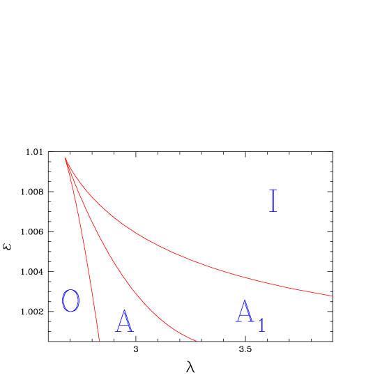
Figure 1: The two dimensional parameter space division for low angular momentum axisymmetric accretion in the Kerr metric. The parameter space is spanned by the conserved specific energy of the flow ${\cal E}$ and the specific angular momentum $\lambda$, and has been drawn for a fixed value of $\gamma=4/3$ and $a=0.3$. The O and the I regions represents the mono-critical mono-transonic accretion solutions passing through the saddle type outer and the inner critical (sonic) points, respectively. The region marked by A represents multi-critical accretion, and can further be divided (not shown in the figure) into two different regions, ${\bf A_{\sf NS}}$ where shock does not form even if the flow has three critical points, and ${\bf A_{\sf S}}$, which accommodates true multi-transonic accretion with general relativistic Rankine Hugoniot shock. The region marked by ${\bf A_{1}}$ represents mono-transonic accretion passing through the inner sonic point and accompanied by an additional pair of non-accessible critical points and a homoclinic orbit through one of those, see text for further details.

4 March toward the multi-transonicity

4.1 The parameter space diagram

By substituting the value of the bulk velocity and the acoustic velocity evaluated at the critical points to the expression for the energy first integral, one obtains a quasi polynomial (not an exact polynomial in strict mathematical sense, since it contains fractional power terms) in $r_{c}$ parametrized by $\left[{\cal E},\lambda,\gamma,a\right]$. Solution of such a quasi polynomial (with additional physical constraint that all solutions must be real, positive and will be greater than $r_{g}$), provides the critical points for general relativistic axisymmetric accretion in the Kerr metric. One finds at most three critical points for relativistic disc accretion for some values of $\left[{\cal E},\lambda,\gamma,a\right]$.

The above mentioned quasi polynomial, and hence the critical points, are completely determined by four parameters $\left[{\cal E},\lambda,\gamma,a\right]$. A four dimensional parameter hyper-space is thus required to be looked upon to obtain the global set of transonic solutions. For the shake of convenience, we analyze a two dimensional projection of such four dimensional hyperspace. Since ${\cal E},\lambda,\gamma,a$ are mutually orthogonal (i.e., choice of one among those four parameters does not influence the choice of the other parameter(s)), a total number of ${}^{4}C_{2}$ different choices are allowed for selecting such projections, each characterized with two different parameters out of the four parameter set $\left[{\cal E},\lambda,\gamma,a\right]$, by keeping the other two parameters at a pre defined fixed value. In this work, we choose to project the hyperspace on an $\left[{\cal E}-\lambda\right]$ plane by keeping $\gamma=4/3$ and $a=0.3$. However, similar projected $\left[{\cal E}-\lambda\right]$ submanifold can routinely be analyzed for other values of $\gamma$ and $a$.

To begin with, we first set the astrophysically relevant bounds on $\left\{{\cal E},{\gamma}\right\}$ to model the realistic situations encountered in astrophysics. Since the specific energy ${\cal E}$ includes the rest-mass energy, ${\cal E}=1$ is the lower bound which corresponds to a flow with zero thermal energy at infinity. Hence, the values ${\cal E}<1$, corresponding to the negative energy accretion states, would be allowed if a mechanism for a radiative extraction of the rest-mass energy existed. The possibility of such an extraction would in turn imply the presence of the viscosity or other dissipative mechanisms in the fluid. Since we concentrate only on non-dissipative flows, we exclude ${\cal E}<1$. On the other hand, although almost all ${\cal E}>1$ are theoretically allowed, large values of ${\cal E}$ represent flows starting from infinity with very high thermal energy. In particular, ${\cal E}>2$ accretion represents enormously hot flow configurations at very large distance from the black hole, which are not properly conceivable in realistic astrophysical situations. Hence, we set $1{\lower 2.15277pt\hbox{$\;\buildrel<\over{\sim}\;$}}{\cal E}{\lower 2.15277pt\hbox{$\;\buildrel<\over{\sim}\;$}}2$.

The physical lower bound on the polytropic index is $\gamma=1$, which corresponds to isothermal accretion where accreting fluid remains optically thin. Hence, the values $\gamma<1$ are not realistic in accretion astrophysics. On the other hand, $\gamma>2$ is possible only for superdense matter with a very large magnetic field and a direction-dependent anisotropic pressure. The presence of a magnetic field would in turn require solving the general relativistic magneto-hydrodynamic equations, which is beyond the scope of this paper. Thus, we set $1{\lower 2.15277pt\hbox{$\;\buildrel<\over{\sim}\;$}}\gamma{\lower 2.15277pt\hbox{$\;\buildrel<\over{\sim}\;$}}2$. However, astrophysically preferred values of $\gamma$ for realistic black-hole accretion range from $4/3$ (ultra-relativistic) to $5/3$ (purely non-relativistic flow) (Frank et al., 2002). Hence, we mainly focus on the parameter range

$$\left[1{\lower 2.15277pt\hbox{$\;\buildrel<\over{\sim}\;$}}{\cal E}{\lower 2.15277pt\hbox{$\;\buildrel<\over{\sim}\;$}}2,~{}\frac{4}{3}{\leq}\gamma{\leq}\frac{5}{3}\right].$$ (33)

In figure 1, the regions marked by O and I correspond to the formation of a single critical point, and hence the mono-transonic disc accretion is produced for such region. In the region marked by I, the critical points are called ‘inner type’ critical points since these points are formed sufficiently close to the event horizon, in most of the cases even closer than the innermost stable circular orbit (ISCO). In the region marked by O, the critical points are called ‘outer type’ critical points, because these points are located relatively far from the black hole. Depending on the value of $\left[{\cal E},\lambda,\gamma,a\right]$, an outer critical point may be as far as $10^{6}r_{g}$, or more.

The outer type critical points for the mono-transonic region are formed, as is obvious from the figure, for sufficiently weakly-rotating flows. For sufficiently low angular momentum, accretion flow contains less amount of rotational energy, thus most of the kinetic energy in utilized to increase the radial dynamical velocity $u$ at a faster rate, leading to a higher value of $du/dr$. Under such circumstances, the dynamical velocity $u$ becomes large enough to overcome the acoustic velocity $c_{s}$ at a larger radial distance from the event horizon, leading to the generation of supersonic flow at a large value of $r$, which results the formation of the sonic point (and hence the corresponding critical point) far away from the black hole event horizon. On the contrary, the inner type critical points are formed, as is observed from the figure, for strongly rotating flow in general. Owing to the fact that such flow would posses a large amount of rotational energy, only a small fraction of the total specific energy of the flow will be spent to increase the radial dynamical velocity $u$. Hence for such flow, $u$ can overcome $c_{s}$ only at a very small distance (very close to the event horizon) where the intensity of the gravitational field becomes enormously large, producing a very high value of the linear kinetic energy of the flow (high $u$), over shedding the contribution to the total specific energy from all other sources. However, from the figure it is also observed that the inner type sonic points are formed also for moderately low values of the angular momentum as well (especially in the region close to the vertex of the wedge shaped zone marked by ${\sf A_{1}}$). For such regions, the total conserved specific energy is quite high. In the asymptotic limit, the expression for the total specific energy is governed by the Newtonian construct, and one can have:

$${\cal E}=\left(\frac{u^{2}}{2}\right)_{\rm linear}+\left(\frac{c_{s}^{2}}{\gamma-1}\right)_{\rm thermal}+\left(\frac{\lambda^{2}}{2r^{2}}\right)_{\rm rotational}+\left(\Phi\right)_{\rm gravitational}$$ (34)

where $\Phi$ is the gravitational potential energy in the asymptotic limit. From (34) it is obvious that at a considerably large distance from the black hole, the contribution to the total energy of the flow comes mainly (rather entirely) from the thermal energy. A high value of ${\cal E}$ (flow energy in excess to its rest mass energy) corresponds to a ‘hot’ flow starting from infinity. Hence the acoustic velocity corresponding to the ‘hot’ flow obeying such outer boundary condition would be quite large. For such accretion, flow has to travel a large distance subsonically and can acquire a supersonic dynamical velocity $u$ only at a very close proximity to the event horizon, where the gravitational pull would be enormously strong.

The $\left[{\cal E},\lambda\right]$ corresponding to the wedge shaped regions marked by A and ${\sf A_{1}}$ produces three critical points, among which the largest and the smallest values correspond to the saddle type, the outer $r_{c}^{out}$ and the inner $r_{c}^{in}$, critical points respectively. The centre type middle critical point, $r_{c}^{mid}$, which is unphysical in the sense that no steady transonic solution passes through it, lies in between $r_{c}^{in}$ and $r_{c}^{out}$.

For the kind of accretion flow considered in this work, the critical points of the phase trajectories can be identified first, following which a linearized study in the neighbourhood of these critical points may be carried out, to develop a complete and rigorous mathematical classification scheme to identify whether a critical point is of saddle type or of centre type. Global understanding of the flow topologies will then necessitate a full numerical integration of the non-linear equations of the flow, which has successfully been performed in this work. For the shake of completeness and to have a better understanding of the multi-transonic behaviour, it will not be unjustified to briefly discuss the classification scheme for the various kind of critical points which may be produced in relativistic accretion disc around a Kerr black hole. Following Goswami et al. (2007), the methodology for performing such classification is presented below.

4.2 Classification scheme for the critical points

Eq. (26) could be reformulated as

$$\frac{du^{2}}{dr}={\frac{\frac{2}{\gamma+1}c_{s}^{2}\left[\frac{g^{\prime}_{1}}{g_{1}}-\frac{1}{g_{2}}\frac{\partial g_{2}}{\partial r}\right]-\frac{f^{\prime}}{f}}{\frac{1}{1-u^{2}}\left(1-\frac{2}{\gamma+1}\frac{c_{s}^{2}}{u^{2}}\right)+\frac{2}{\gamma+1}\frac{c_{s}^{2}}{g_{2}}\left(\frac{\partial g_{2}}{\partial u^{2}}\right)}}$$ (35)

$$\frac{du^{2}}{d{\bar{\tau}}}=\frac{2}{\gamma+1}c_{s}^{2}\left[\frac{g^{\prime}_{1}}{g_{1}}-\frac{1}{g_{2}}\frac{\partial g_{2}}{\partial r}\right]-\frac{f^{\prime}}{f}$$ (36)

with the primes representing the total derivatives with respect to $r$, and $\bar{\tau}$ is an arbitrary mathematical parameter. Here,

$$f(r)=\frac{Ar^{2}\Delta}{A^{2}-4\lambda arA+\lambda^{2}r^{2}(4a^{2}-r^{2}\Delta)},~{}$$

$$g_{1}(r)=\Delta r^{4},~{}g_{2}(r,u)=\frac{\lambda^{2}f}{1-u^{2}}-\frac{a^{2}f^{\frac{1}{2}}}{\sqrt{1-u^{2}}}+a^{2}$$ (37)

The critical conditions are obtained with the simultaneous vanishing of the right hand side, and the coefficient of ${d(u^{2})/dr}$ in the left hand side in (35). This will provide

$$\left|\frac{2c_{s}^{2}}{\gamma+1}\left[\frac{g_{1}^{\prime}}{g_{1}}-\frac{1}{g_{2}}\left(\frac{\partial{g_{2}}}{\partial{r}}\right)\right]-\frac{f^{\prime}}{f}\right|_{\rm r=r_{c}}=\left|\frac{1}{1-u^{2}}\left(1-\frac{2}{\gamma+1}\frac{c_{s}^{2}}{u^{2}}\right)+\frac{2}{\gamma+1}\frac{c_{s}^{2}}{g_{2}}\left(\frac{\partial{g_{2}}}{\partial{u^{2}}}\right)\right|_{\rm r=r_{c}}=0$$ (38)

as the two critical point conditions. Some simple algebraic manipulations shows that

$$u_{c}^{2}=\frac{f^{\prime}g_{1}}{f{g_{1}^{\prime}}},$$ (39)

following which $c_{s}^{2}|_{\rm r=r_{c}}$ can be rendered as a function of $r_{c}$ only, and further, by use of (22)., $r_{c}$, $c_{sc}^{2}$ and $u_{c}^{2}$ can all be fixed in terms of the constants of motion like ${\cal E}$, $\gamma$, $\lambda$ and $a$. Having fixed the critical points it should now be necessary to study their nature in their phase portrait of $u^{2}$ versus $r$. To that end one applies a perturbation about the fixed point values, going as,

$$u^{2}=u^{2}|_{\rm r=r_{c}}+\delta{u^{2}},~{}c_{s}^{2}=c_{s}^{2}|_{\rm r=r_{c}}+\delta{c_{s}^{2}},~{}r=r_{c}+\delta{r}$$ (40)

in the parametrized set of autonomous first-order differential equations,

$$\frac{d({u^{2}})}{d{\bar{\tau}}}=\frac{2}{\gamma+1}c_{s}^{2}\left[\frac{g_{1}^{\prime}}{g_{1}}-\frac{1}{g_{2}}\left(\frac{\partial{g_{2}}}{\partial{r}}\right)\right]\frac{f^{\prime}}{f}$$ (41)

and

$$\frac{dr}{d{\bar{\tau}}}=\frac{1}{1-u^{2}}\left(1-\frac{2}{\gamma+1}\frac{c_{s}^{2}}{u^{2}}\right)+\frac{1}{\gamma+1}\frac{c_{s}^{2}}{g_{2}}\left(\frac{\partial{g_{2}}}{\partial{u^{2}}}\right)$$ (42)

with ${\bar{\tau}}$ being an arbitrary parameter. In the two equations above $\delta c_{s}^{2}$ can be closed in terms of $\delta u^{2}$ and $\delta r$ with the help of (25). Having done so, one could then make use of solutions of the form, $\delta r\sim\exp({\bar{\Omega}}\tau)$ and $\delta u^{2}\sim\exp({\bar{\Omega}}\tau)$, from which, ${\bar{\Omega}}$ would give the eigenvalues — growth rates of $\delta u^{2}$ and $\delta r$ in ${\bar{\tau}}$ space — of the stability matrix implied by (41-42). Detailed calculations will show the eigenvalues to be

$${\bar{\Omega}}^{2}=\left|{\bar{\beta}}^{4}c_{s}^{4}\chi_{1}^{2}+\xi_{1}\xi_{2}\right|_{\rm r=r_{c}}$$ (43)

where ${\bar{\beta}}^{2}=\frac{2}{\gamma+1}$ and $\chi_{1},\xi_{1}$ and $\xi_{2}$ can be expressed as polynomials of $r_{c}$. ${\bar{\Omega}}^{2}$ can be evaluated for any $\left[{\cal E},\lambda,\gamma,a\right]$once the value of the corresponding critical point $r_{c}$ is known. The structure of (43) immediately shows that the only admissible critical points in the conserved Kerr system will be either saddle points or centre type points. For a saddle point, ${\bar{\Omega}}^{2}>0$, while for a centre-type point, ${\bar{\Omega}}^{2}<0$.

For multi-critical flow characterized by a specific set of $\left[{\cal E},\lambda,\gamma,a\right]$, one can obtain the value of ${\bar{\Omega}}^{2}$ to be positive for the inner and the outer critical points, showing that those critical points are of saddle type in nature. ${\bar{\Omega}}^{2}$ comes out to be negative for the middle critical point, confirming that the middle critical point is of centre type and hence no transonic solution passes through it. One can also confirm that all mono-transonic flow (flow with a single critical point characterized by $\left[{\cal E},\lambda\right]$ taken either from I or from O region) corresponds to saddle type critical point.

4.3 Distinction between the two different category of flows, both having three distinct critical points

There are distinct topological differences between the multi-transonic flow characterized by $\left[{\cal E},\lambda\right]$ taken from the region marked by A, and the region marked by ${\bf A_{1}}$. For region marked by A, the entropy accretion rate ${\dot{\Xi}}$ for flows passing through the inner critical point is greater than that of the outer critical point

$${\dot{\Xi}}\left(r_{c}^{in}\right)>{\dot{\Xi}}\left(r_{c}^{out}\right)$$ (44)

while for the region marked by ${\bf A_{1}}$, the following relation holds

$${\dot{\Xi}}\left(r_{c}^{in}\right)<{\dot{\Xi}}\left(r_{c}^{out}\right)$$ (45)

The above two relations show that $\left[{\cal E},\lambda\right]$ region marked by A represents the possibility of having multi-critical multi-transonic accretion, while $\left[{\cal E},\lambda\right]{\in}\left[{\cal E},\lambda\right]_{\bf A_{1}}$ corresponds to the mono-transonic accretion, with an additional pair of critical points. For the multi-critical accretion, as we will see in more detail in the subsequent sections, and as is illustrated in the panel diagrams (ii) - (iv) of figure 2, one can have a possibility that the global accretion solution may pass through the outer critical/sonic point, and a local accretion solution passing through the inner critical/sonic point, which folds back onto itself (at a point of inflexion formed at a certain radial distance $r{\equiv}r\left({\cal E},\lambda,\gamma,a\right)$), forming a homoclinic orbit passing through the saddle type inner critical point and embracing the centre type middle critical point flanked by the saddle type outer and the inner critical points. Such a homoclinic orbit can be connected with the standard non-homoclinic path through a standing shock, and hence, for a suitable initial boundary condition determined by $\left[{\cal E},\lambda,\gamma,a\right]$, accretion flow can pass through both the inner and the outer saddle type critical/sonic points. Hence we designate such flows (characterized by the set of parameters taken from the region A of the parameter space, as shown in figure 1), which can have more than one sonic point available to it to pass through (in reality whether it will pass through both the sonic points depends on the possibility of the shock formation, see subsequent sections for further details) to be ‘multi-transonic’ accretion.

The region A, thus, as we will further discuss in the subsequent sections in even more details, can further be divided into two regions. For the region where three critical points exist but no shock solution is allowed, the accretion is of the category multi-critical mono-transonic in strict sense, and such a region will hereafter be marked as ${\bf A_{\sf NS}}$ – which reads ‘multi-critical mono-transonic accretion flow with no shock’. For the rest of the A region, a steady standing Rankine Hugoniot kind of shock forms, and accretion passes through both of the outer and the inner sonic points. Accretion is thus truly multi-transonic, and such a region in parameter space will be marked as ${\bf A_{\sf S}}$, which reads ‘multi-critical multi-transonic accretion with shock’.

On the other hand, flows described by the parameters taken from the region ${\bf A_{1}}$ of the parameter space behaves in a completely different way. Here, the global accretion solution passes through the inner critical/sonic point and hence it is mono-transonic. The homoclinic orbit is formed through the outer critical point, and the accretion sector of such homoclinic orbit can not be connected with the corresponding standard transonic accretion solution passing through the inner sonic point, by a shock (or through by whatever physical means), since the corresponding segment (lying in the length scale spanning the region between the outer critical point and the point of inflexion of the homoclinic loop) of the global transonic solution remains subsonic (shock can not form in a subsonic flow). We thus call such flow topologies as the ‘mono-transonic accretion with an additional pair of critical points’.

It is to be noted that the above mentioned solutions are commonly known as the ’multi-transonic wind’ in the literature, owing to the fact that for a limited subset of values of $\left[{\cal E},\lambda,\gamma,a\right]$ taken from the region ${\bf A_{1}}$, the wind segment of the homoclinic orbit can be connected to the non homoclinic wind like solutions (passing through the inner sonic point) through a standing shock. However, we would not like to use such terminology here. Such terminology, as we feel, is misleading in the sense that the wind solution have no role in studying the accretion phenomena (except, perhaps, for studying the accretion powered outflow), and hence the term ‘multi-transonic wind’ sounds as if there is no accretion taking place for the initial boundary conditions chose from the region ${\bf A_{1}}$, and such nomenclature is of compromised clarity only.

The actual situation, in contrary, is that there are several phases of transonic accretion flow, as we see in the subsequent section, and we concentrate only on the accretion part when we study accretion onto the black holes. The only true multi-transonic accretion are obtained if and only if shocks are formed. Otherwise, the accretion is always mono-transonic, whether the flow possesses more than one critical points or not. Either such mono-transonic solution has only one saddle type critical point, and one corresponding sonic point (outer or inner), or it can have two sonic points available, and a homoclinic orbit passing through the inner critical point, but due to the absence of the shock formation phenomena, the transonic flow is realizable only through the outer sonic point, and the flow is essentially topologically isomorphic to the mono-critical mono-transonic accretion from the region marked by O in the parameter space as shown in the figure 1, or, in its last variant, the flow can have three critical points, but the transonic accretion passes through only through the inner critical/sonic point, accompanied by a homoclinic loop through the outer critical point, and the corresponding accretion flow configuration is isomorphic to the mono-critical mono-transonic accretion passing through the inner critical/sonic point, as observed for flows chosen from the region marked by I in the parameter space as shown in the figure 1. All such issues will be further clarified in greater detail in the next section.

The boundary between the region marked by A and ${\bf A_{1}}$ is a very special one, since for $\left[{\cal E},\lambda\right]$ defined by the boundary, the entropy accretion rate corresponding to the solution passing through the outer critical point is exactly same as that of through the inner critical point (${\dot{\Xi}}\left(r_{c}^{in}\right)={\dot{\Xi}}\left(r_{c}^{out}\right)$). $\left[{\cal E},\lambda\right]$ defined by this boundary (rather $\left[{\cal E},\lambda,\gamma\right]$ for a fixed $a$, defined by this surface in general) provides the non-removable degenerate bistable/unstable solutions, we will discuss this issue in more details later.

There are other regions for $\left[{\cal E},\lambda\right]$ space for which either no critical points are formed, or two critical points are formed. These regions are not shown in the figure, since none of these regions is of our interest. If no critical point is found, it is obvious that transonic accretion does not take place for those set of $\left[{\cal E},\lambda\right]$. For two critical point region, one of the critical points are always of centre type, since according to the standard dynamical systems theory two successive critical points can not be of same type (both saddle, or both centre). Hence the solution which passes through the saddle type critical point would encompass the centre type critical point by forming a loop like homoclinic orbit, and hence such solution would not be physically acceptable accretion solutions since such solutions do not connect infinity to the event horizon. In subsequent sections, we will thoroughly describe the methodology for obtaining such flows parametrized by $\left[{\cal E},\lambda,\gamma,a\right]$ taken from the regions A and ${\bf A_{1}}$.

Figure 2: Solution topologies for various cases as obtained by gradually increasing the flow angular momentum, by keeeping the other initial boundary conditions at a fixed value of $\left[{\cal E}=1.0000033,\gamma=4/3,a=0.3\right]$. The usual accretion branch is denoted by solid line (red coloured in the online version) marked by ‘Acc’, and the other solid line intersecting the accretion branch (at the outer critical points for panel (ii) - (iv) and at the inner critical point at panel (vi)) represents the corresponding wind solution. The homoclinic orbit passing through the inner (for panel (ii) - (iv) ) or the outer (for panel (vi)) critical point is shown by the dotted line (blue coloured in the online version). The shock transition (at panel (iv) for true multi-transonic accretion, and at panel (vi) for shock formation in wind solution) is shown by vertical long dashed line (green coloured in the online version).

5 Effect of change of the control parameter on the phase portrait

5.1 Mono-transonic flow: Characteristics of the integral curves and the methodology to obtain the flow topology

As has already been mentioned, we choose an $\left[{\cal E}-\lambda\right]$ projection of the entire four dimensional parameter space. The transonic flow properties and the corresponding flow topologies depends on four parameters of the $\left[{\cal E},\lambda,\gamma,a\right]$set. We would like to illustrate such dependence by varying one parameter while keeping the other three parameters fixed. We will smoothly vary the angular momentum $\lambda$ of the flow and will observe its consequence on the phase topology. The corresponding topologies have been shown in six different panels (i) – (vi) in figure 2. All the panel figures are drawn by plotting the Mach number along the Y axis and the distance (measured from the event horizon and scaled in the unit of the gravitational radius) along the X axis in logarithmic scale. For all the topologies in the figure, the value of ${\cal E}$ has been chosen to be $1.0000033$, which is in accordance with the value of the Bernoulli’s constant for accretion flow onto the supermassive black hole located at our Galactic centre Moscibrodzka, Das & Czerny (2006). The value of $\gamma$ has routinely been taken to be $4/3$, and $a=0.3$ has been taken as a representative value of the Kerr parameter. Same procedure can be performed using any other value of $a$ as well. Stable mono-transonic global solutions through the outer critical point is available for $0<\lambda{\leq}\lambda_{1}$, where $\lambda_{1}$ has the value in between 2.839 and 2.84. For such an interval of $\lambda$, the solution topology has been shown in the panel (i) of the figure 2, hereafter described as panel (ii).

We now describe (in somewhat great detail) the methodology for obtaining a transonic solution topology on a phase portrait. This requires numerical integration of the equations describing the velocity gradient, as well as the gradient of the acoustic velocity, of the accretion flow. One thus needs to define the value of both the velocity gradients at the critical point, pick up the required quantities (the value of the dynamical and the acoustic velocities, and their respective gradients at the critical point, and of the critical point itself), and to use those values as the starting values for the integration, like what is to be done in case of the standard initial value problem corresponding to the numerical solution of the differential equation.

To obtain the dynamical velocity gradient at the critical point, one applies l’Hospital’s rule on (26). After some algebraic manipulations, the following quadratic equation is formed, which can be solved to obtain $(du/dr)_{\bf{{|_{(r=r_{c})}}}}$ (see Barai et al. (2004) for further details):

$$\alpha\left(\frac{du}{dr}\right)_{\bf{{|_{(r=r_{c})}}}}^{2}+\beta\left(\frac{du}{dr}\right)_{\bf{{|_{(r=r_{c})}}}}+\zeta=0,$$ (46)

where the coefficients are:

$$\alpha=\frac{\left(1+u^{2}\right)}{\left(1-u^{2}\right)^{2}}-\frac{2\delta_{1}\delta_{5}}{\gamma+1},\quad\quad\beta=\frac{2\delta_{1}\delta_{6}}{\gamma+1}+\tau_{6},\quad\quad\zeta=-\tau_{5};$$

$$\delta_{1}=\frac{c_{s}^{2}\left(1-\delta_{2}\right)}{u\left(1-u^{2}\right)},\quad\quad\delta_{2}=\frac{u^{2}v_{t}\sigma}{2\psi},\quad\quad\delta_{3}=\frac{1}{v_{t}}+\frac{2\lambda^{2}}{\sigma}-\frac{\sigma}{\psi},\quad\quad\delta_{4}=\delta_{2}\left[\frac{2}{u}+\frac{uv_{t}\delta_{3}}{1-u^{2}}\right],$$

$$~{}\delta_{5}=\frac{3u^{2}-1}{u\left(1-u^{2}\right)}-\frac{\delta_{4}}{1-\delta_{2}}-\frac{u\left(\gamma-1-c_{s}^{2}\right)}{a_{s}^{2}\left(1-u^{2}\right)},\quad\quad\delta_{6}=\frac{\left(\gamma-1-c_{s}^{2}\right)\chi}{2c_{s}^{2}}+\frac{\delta_{2}\delta_{3}\chi v_{t}}{2\left(1-\delta_{2}\right)},$$

$$\tau_{1}=\frac{r-1}{\Delta}+\frac{2}{r}-\frac{\sigma v_{t}\chi}{4\psi},\quad\quad\tau_{2}=\frac{\left(4\lambda^{2}v_{t}-a^{2}\right)\psi-v_{t}\sigma^{2}}{\sigma\psi},$$

$$\tau_{3}=\frac{\sigma\tau_{2}\chi}{4\psi},\quad\quad\tau_{4}=\frac{1}{\Delta}-\frac{2\left(r-1\right)^{2}}{\Delta^{2}}-\frac{2}{r^{2}}-\frac{v_{t}\sigma}{4\psi}\frac{d\chi}{dr},$$

$$\tau_{5}=\frac{2}{\gamma+1}\left[c_{s}^{2}\tau_{4}-\left\{\left(\gamma-1-c_{s}^{2}\right)\tau_{1}+v_{t}c_{s}^{2}\tau_{3}\right\}\frac{\chi}{2}\right]-\frac{1}{2}\frac{d\chi}{dr},$$

$$\tau_{6}=\frac{2v_{t}u}{\left(\gamma+1\right)\left(1-u^{2}\right)}\left[\frac{\tau_{1}}{v_{t}}\left(\gamma-1-c_{s}^{2}\right)+c_{s}^{2}\tau_{3}\right].$$ (47)

Note that all the above quantities are evaluated at the critical point.

Hence we compute the critical advective velocity gradient as

$$\left(\frac{du}{dr}\right)_{\rm r=r_{c}}=-\frac{\beta}{2\alpha}{\pm}\sqrt{\beta^{2}-4\alpha{\zeta}}$$ (48)

where the ‘+’ sign corresponds to the accretion solution and the ‘-’ sign corresponds to the wind solution, see the following discussion for further details. Similarly, the space gradient of the acoustic velocity $dc_{s}/dr$ and its value at the critical point has also been calculated.

For the solution topologies shown in the figure 2, using the specified set of $\left[{\cal E},\lambda,\gamma,a\right]$, we first solve the equation for the energy first integral defined at the critical point, to obtain the corresponding critical point $r_{c}=99851.8623$, which is the point of intersection in between the accretion branch marked by ‘Acc’ in the figure, and the corresponding wind branch, the other curve shown in the figure. We then calculate the critical value of the advective velocity gradient at $r_{c}$ from (48). By integrating the equation for the dynamical and the acoustic flow velocity gradient (Eq. (25) and (26), respectively), from the critical point, using the fourth-order Runge-Kutta method, we then calculate the local advective velocity, the polytropic sound speed, the Mach number, the fluid density, the disc height, the bulk temperature of the flow, and any other relevant dynamical and thermodynamic quantity characterizing the flow. In this way we obtain the accretion branch ‘Acc’ by employing the above mentioned procedure.

The solution, as is obvious from the figure, is two-fold degenerate owing to the $\pm u$ degeneracy which reflects the physical accretion/wind degeneracy. We have, however, removed the degeneracy by orienting the curves, and thus each line represents either the wind or accretion. We have arbitrarily assigned the $+$ sign solution in Eq. (48) to the accretion and the $-$ sign solution in Eq. (48) to the ‘wind’ branch. This wind branch is just a mathematical counterpart of the accretion solution (velocity reversal symmetry of accretion), owing to the presence of the quadratic term of the dynamical velocity in the equation governing the energy momentum conservation.

The term ‘wind solution’ has a historical origin. The solar wind solution first introduced by Parker  (Parker, 1965) has the same topology profile as that of the wind solution obtained in classical Bondi accretion  (Bondi, 1952). Hence the name ‘wind solution’ has been adopted in a more general sense. The wind solution thus represents a hypothetical process, in which, instead of starting from infinity and heading towards the black hole, the flow generated near the black-hole event horizon would fly away from the black hole towards infinity. The topology of such a process is represented by the wind solution in the panel, which, as already been mentioned, is the curve intersecting the accretion branch ‘Acc’ at the outer critical point.

The above procedure for obtaining the flow topology is also applied to draw the mono-transonic accretion/wind branch through the inner sonic point. In fact, the same procedure may be used to draw real physical transonic accretion/wind solutions passing through any acceptable saddle-type critical point. Note, however, that the sector of the accretion branch starting from the intersection of the accretion and the wind solution in the panel diagram and ending at the event horizon is not the complete subsonic branch, because the point of intersection is a critical point and not a sonic point. Using the procedure described above we have to integrate the flow from the critical point to the sonic point where the Mach number becomes unity.

5.2 Appearance of the homoclinic orbit and the emergence of the multi-transonicity

We now further increase $\lambda$ so as to reach a value $\lambda_{2}$ – greater than but infinitesimally close to $\lambda_{1}$, i.e.:

$${\large\sf Lt}_{{\epsilon}{\rightarrow}0}~{}|\lambda_{2}-\lambda_{1}|=\epsilon$$

$\lambda_{2}$ thus characterizes the flow topology generated at the right side of the boundary between the O and the A regions shown in figure 1, and infinitesimally close to it. Such solution has been shown in the panel (ii). The line separating the O and the A region is actually the line of bifurcation of the critical point, because the number of critical point increases after crossing such line. The line of separation between the O - A region, in general, is a three dimensional hypersurface for the generic multi dimensional parameter space spanned by $\left[{\cal E},\lambda,\gamma,a\right]$. Additional critical points appear in pairs once such a line is crossed from the left side (by gradually increasing the value of the flow angular momentum $\lambda$) of the parameter space. Hence, while increasing $\lambda$ smoothly, initially there is a region of a single saddle point, then followed by the pair creation of a saddle and a centre type point after crossing the O - A boundary. That is what is manifested in panel (ii). In addition to a transonic accretion solution passing through the outer critical point, which is denoted by the solid lines (red coloured in the online version) a tiny loop of homoclinic orbit (shown using dotted line, blue coloured in the online version) appears representing the flow through (and around) a nascent saddle-centre pair of critical points. Physically, this is what it has to be, because with a centre type point but without another saddle point, the flow solutions will all curl about the centre type point, and there will be no means of connecting the event horizon with infinity through an isolated solution passing through the saddle type inner critical point, and embracing the centre type middle critical point (here, the inner and the middle critical points are formed at 7.2 and 7.4 $r_{g}$, respectively). The homoclinic path has its existence in isolation, and unlike the transonic solution passing through the outer critical point, can not be regarded as a global transonic solution on its own. A physically acceptable flow through the inner critical point has to be connected with the solution passing through the outer critical point. As we will see in the subsequent paragraphs, a standing Rankine-Hugoniot shock perfectly accomplish the task.

Accretion flow through the inner critical point has higher value of the entropy accretion rate compared to that of passing through the outer critical point. The ratio ${\sf R}_{\dot{\Xi}}$ of ${\dot{\Xi}}_{in}$ and ${\dot{\Xi}}_{out}$ attains its maximum value close to the O – A boundary, and then monotonically decreases as one smoothly transits to the higher end of $\lambda$ (toward the boundary separating the A and the ${\bf A_{1}}$ regions, respectively).

As we further process toward higher value of $\lambda$, the area enclosed within the homoclinic orbit starts increasing and finally it fills up the entire region bounded by the transonic accretion and wind passing through the outer critical point. The situations have been demonstrated sequentially in the successive panel figures (iii), (iv) and (v).

5.3 Multi-critical accretion with and without shock

In panel (iii), ${\sf R}_{\dot{\Xi}}$ is 212.52. Shock, however, does not form even if three critical points are present. Such multi-critical flow (which is actually a mono-transonic accretion because in absence of the shock, accretion flow can pass only through the outer sonic point even if the inner sonic point formally exists) without a standing shock is observed for a range of value of $\lambda_{2}{\leq}\lambda{\leq}\lambda_{3}$ where $\lambda_{3}{\sim}3.23{\dot{9}}$, which defines the boundary of the ${\bf A_{\sf NS}}$ region.

As $\lambda$ is further increased so that $\lambda>\lambda_{3}$, Rankine-Hugoniot conditions (relativistic Rankin-Hugoniot conditions are explicitly derived in the next section) gets satisfied, and standing shock forms. Panel (iv) shows the topology of the multi-transonic accretion with shock solutions, where the shock transition has been marked by the vertical long-dashed (green coloured in the online version) line segment. The shock location, shock strength, in which is defined as the pre (-) to the post (+) shock ratio (defined not in the temporal sequence but in the spatial sequence, of the Mach number) and is denoted by $M_{-}/M_{+}$, and the entropy enhancement ratio at the shock ${\sf R}_{\dot{\Xi}}$ are found to be 18.3336735 and 74.9621923, respectively.

It is to be noted that the panel (iv) is not the solution corresponding to the minimum value of $\lambda$ for which the shock forms, i.e., does not correspond to the value of $\lambda$ separating the ${\bf A_{\sf NS}}$ and the ${\bf A_{\sf S}}$ region. The strongest shock (forms for the maximally allowed value of ${\sf R_{\dot{\Xi}}}$ in ${\bf A_{\sf S}}$) are formed for $\lambda_{4}$ where

$${\sf Lt}_{\epsilon{\rightarrow}0}|\lambda_{4}-\lambda_{3}|=\epsilon$$

For example, for $\lambda=3.24$, the shock forms at 27.5$r_{g}$, and the corresponding shock strength and the entropy enhancement ratio at the shock are found to be 41.7 and 197.62, respectively.

The relativistic shock equations and its derivation, along with a detail description of the methodology of finding the multi-transonic flow with and without shock is presented in the subsequent paragraphs. However, from panel (iii) and (iv), it is to be understood that shock does not necessarily form for all multi-critical flow. Having two saddle type critical points is thus a necessary but not a sufficient condition. The reason behind this disparity will be analytically justified in the section (6) and section (7)

5.4 Methodology for obtaining multi-transonic topology

Using a specific set of $\left[{\cal E},\lambda,\gamma,a\right]$, one first solves the equation for ${\cal E}$ at the critical point to find out the corresponding three critical points, saddle type inner, centre type middle, and the saddle type outer. The space gradient of the flow velocity as well as the acoustic velocity at the saddle type critical point is then obtained. Such $u_{\bf{{|_{(r=r_{c})}}}},{c_{s}}_{\bf{{|_{(r=r_{c})}}}}$,$dc_{s}/dr_{\bf{{|_{(r=r_{c})}}}}$ and $du/dr_{\bf{{|_{(r=r_{c})}}}}$ serve as the initial value condition for performing the numerical integration of the advective velocity gradient using the fourth-order Runge-Kutta method. Such integration provides the outer sonic point (located closer to the black hole compared to the outer critical point, since the Mach number at the outer critical point is less than unity), the local advective velocity, the polytropic sound speed, the Mach number, the fluid density, the disc height, the bulk temperature of the flow, and any other relevant dynamical and thermodynamic quantity characterizing the flow. The corresponding wind solution through the outer sonic point is obtained in the same way, by taking the other value (note that being a quadratic algebraic equation, solution of (48) provides two initial values, one for the accretion and the other for the wind) of $du/dr_{\bf{{|_{(r=r_{c})}}}}$.

The respective accretion and the wind solutions passing through the inner critical point are obtained following exactly the same procedure as has been used to draw the accretion and wind topologies passing through the outer critical point. Note, however, that the accretion solution through the inner critical point folds back onto the wind solution which is a homoclinic orbit through the inner critical point encompassing the centre type middle critical point. A physically acceptable transonic solution must be globally consistent, i.e. it must connect the radial infinity with the black-hole event horizon. Hence, for multi-transonic accretion, there is no individual existence of physically acceptable accretion/wind solution passing through the inner critical (sonic) point, although, depending on the initial boundary conditions, such solution may be clubbed with the accretion solution passing through outer critical point, through a standing shock.

The set $\left[{\cal E},\lambda\right]_{\bf A}$ (or more generally $\left[{\cal E},\lambda,\gamma,a\right]_{\bf A}$) thus produces doubly degenerate accretion/wind solutions. Such two fold degeneracy may be removed by the entropy considerations since the entropy accretion rates for solutions passing through the inner critical point and the outer critical point are generally not equal. For any $\left[{\cal E},\lambda,\gamma,a\right]{\in}\left[{\cal E},\lambda,\gamma,a\right]_{\bf A}$ we find that the entropy accretion rate ${\dot{\Xi}}$ evaluated for the complete accretion solution passing through the outer critical point is less than that of the rate evaluated for the incomplete accretion/wind solution passing through the inner critical point. Since the quantity ${\dot{\Xi}}$ is a measure of the specific entropy density of the flow, the solution passing through the outer critical point will naturally tend to make a transition to its higher entropy counterpart, i.e. the globally incomplete accretion solution passing through the inner critical point. Hence, if there existed a mechanism for the accretion solution passing through the outer critical point to increase its entropy accretion rate exactly by an amount

$${\Delta}{\dot{\Xi}}={\dot{\Xi}}(r_{c}^{\rm in})-{\dot{\Xi}}(r_{c}^{\rm out}),$$ (49)

there would be a transition to the accretion solution passing through the inner critical point. Such a transition would take place at a radial distance somewhere between the radius of the inner sonic point and the radius of the point of inflexion of the homoclinic orbit. In this way one would obtain a true multi-transonic accretion solution connecting the infinity and the event horizon, which includes a part of the accretion solution passing through the inner critical, and hence the inner sonic point. One finds that for some specific values of $\left[{\cal E},\lambda,\gamma,a\right]_{\bf A}$, a standing Rankine-Hugoniot shock may accomplish this task. A supersonic accretion through the outer sonic point (which in obtained by integrating the flow starting from the outer critical point) can generate entropy through such a shock formation and can join the flow passing through the inner sonic point (which in obtained by integrating the flow starting from the outer critical point). Below we will carry on a detail discussion on such shock formation.

5.5 The shock formation and related phenomena

In the present work, the basic equations governing the flow are the energy and baryon number conservation equations which contain no dissipative terms and the flow is assumed to be inviscid. Hence, the shock which may be produced in this way can only be of Rankine-Hugoniot type which conserves energy. The shock thickness must be relatively small in this case, otherwise non-dissipative flows may radiate energy through the upper and the lower boundaries because of the presence of strong temperature gradient in between the inner and outer boundaries of the shock thickness. In the presence of a shock the flow may have the following profile. A subsonic flow starting from infinity first becomes supersonic after crossing the outer sonic point and somewhere in between the outer sonic point and the inner sonic point the shock transition takes place and forces the solution to jump onto the corresponding subsonic branch. The hot and dense post-shock subsonic flow produced in this way becomes supersonic again after crossing the inner sonic point and ultimately dives supersonically into the black hole. A flow heading towards a neutron star can have the liberty of undergoing another shock transition after it crosses the inner sonic point. Or, alternatively, a shocked flow heading towards a neutron star need not encounter the inner sonic point at all. This is because, the hard surface boundary condition of a neutron star by no means prevents the flow from hitting the star surface subsonically.

For the complete general relativistic accretion flow discussed in this article, the energy momentum tensor ${\large\sf T}^{{\mu}{\nu}}$, the four-velocity $v_{\mu}$, and the speed of sound $c_{s}$ may have discontinuities at a hypersurface $\Sigma$ with its normal $\eta_{\mu}$. Using the energy momentum conservation and the continuity equation, we have:

$$\left[\left[{\rho}v^{\mu}\right]\right]{\eta}_{\mu}=0,\left[\left[{\large\sf T}^{\mu\nu}\right]\right]{\eta}_{\nu}=0.$$ (50)

For a perfect fluid, we thus formulate the relativistic Rankine-Hugoniot conditions as

$$\left[\left[{\rho}u\Gamma_{u}\right]\right]=0,$$ (51)

$$\left[\left[{\large\sf T}_{t\mu}{\eta}^{\mu}\right]\right]=\left[\left[(p+\epsilon)v_{t}u\Gamma_{u}\right]\right]=0,$$ (52)

$$\left[\left[{\large\sf T}_{\mu\nu}{\eta}^{\mu}{\eta}^{\nu}\right]\right]=\left[\left[(p+\epsilon)u^{2}\Gamma_{u}^{2}+p\right]\right]=0,$$ (53)

where $\Gamma_{u}=1/\sqrt{1-u^{2}}$ is the Lorentz factor. The first two conditions (51) and (52) are trivially satisfied owing to the constancy of the specific energy and mass accretion rate. The constancy of mass accretion yields

$$\left[\left[K^{-\frac{1}{\gamma-1}}\left(\frac{\gamma-1}{\gamma}\right)^{\frac{1}{\gamma-1}}\left(\frac{c_{s}^{2}}{\gamma-1-c_{s}^{2}}\right)^{\frac{1}{\gamma-1}}\frac{u}{\sqrt{1-u^{2}}}H(r)\right]\right]=0.$$ (54)

The third Rankine-Hugoniot condition (53) may now be written as

$$\left[\left[K^{-\frac{1}{\gamma-1}}\left(\frac{\gamma-1}{\gamma}\right)^{\frac{\gamma}{\gamma-1}}\left(\frac{c_{s}^{2}}{\gamma-1-c_{s}^{2}}\right)^{\frac{\gamma}{\gamma-1}}\left\{\frac{u^{2}\left(\gamma-c_{s}^{2}\right)+c_{s}^{2}}{c_{s}^{2}\left(1-u^{2}\right)}\right\}\right]\right]=0.$$ (55)

Simultaneous solution of Eqs. (54) and (55) yields the ‘shock invariant’ quantity ${\cal S_{h}}$ which changes continuously across the shock surface. We obtain the analytical expression for ${\cal S_{h}}$ in terms of various local accretion variables and initial boundary conditions. The shock location in multi-transonic accretion is found in the following way. While performing the numerical integration along the solution passing through the outer critical point, we calculate the shock invariant ${\cal S}_{h}$ in addition to $u$, $c_{s}$ and $M$. We also calculate ${\cal S}_{h}$ while integrating along the solution passing through the inner critical point, starting from the inner sonic point up to the point of inflexion of the homoclinic orbit. We then determine the radial distance $r_{sh}$, where the numerical values of ${\cal S}_{h}$, obtained by integrating the two different sectors described above, are equal. Generally, for any value of $\left[{\cal E},\lambda,\gamma,a\right]$allowing shock formation, one finds two formal shock locations, one located in between the outer and the middle sonic point and the other one located in between the inner and the middle sonic point. The shock strength is different for the inner and for the outer shock. According to the standard local stability analysis (Yang & Kafatos (1995)), for a multi-transonic accretion, one can show that only the shock formed between the middle and the outer sonic point is stable. Hereafter, whenever we mention the shock location, we always refer to the stable shock location only.

We find that the shock location correlates with $\lambda$. This is obvious because the higher the flow angular momentum, the greater the rotational energy content of the flow. As a consequence, the strength of the centrifugal barrier which is responsible to break the incoming flow by forming a shock will be higher and the location of such a barrier will be farther away from the event horizon. However, the shock location anti-correlates with ${\cal E}$ and $\gamma$. This means that for the same ${\cal E}$ and $\lambda$, in the purely non-relativistic flow the shock will form closer to the black hole compared with the ultra-relativistic flow. Besides, we find that the shock strength anti-correlates with the shock location $r_{sh}$, which indicates that the closer to the black hole the shock forms , the higher the strength and the entropy enhancement ratio are. The ultra-relativistic flows are supposed to produce the strongest shocks. The reason behind this is also easy to understand. The closer to the black hole the shock forms, the higher the available gravitational potential energy must be released, and the radial advective velocity required to have a more vigorous shock jump will be larger. Besides we note that as the flow gradually approaches its purely non-relativistic limit, the shock may form for lower and lower angular momentum, which indicates that for purely non-relativistic accretion, the shock formation may take place even for a quasi-spherical flow. However, it is important to mention that a shock formation will be allowed not for every $\left[{\cal E},\lambda,\gamma,a\right]{\in}\left[{\cal E},\lambda,\gamma,a\right]_{\bf A}$, The numerical value for ${\cal S_{h}}$ will be the same along both the accretion through the outer and the inner sonic point, only at certain points (the shock locations) for a specific subset of $\left[{\cal E},\lambda,\gamma,a\right]_{\bf A}$, for which a steady, standing shock solution will be found.

We further find that the shock location correlates with the black hole spin parameter, whereas the shock strength and the entropy enhancement ratio at the shock anti correlates with the Kerr parameter. The post to pre shock velocity correlates with the black hole spin, whereas the post to pre shock temperature, density and pressure anti correlates with the Kerr parameter.

5.6 The ‘asymmetrically hunched fish’ and the heteroclinic orbits

As we further increase $\lambda$, the shock location recedes outward, and the shock strength as well as ${\sf R}_{\dot{\Xi}}$ decreases monotonically. Meanwhile, the homoclinic path embracing the middle critical point starts filling up the entire region accessible to it. Finally, when $\lambda$ approaches the value $\lambda_{5}{\sim}3.57401752$, the interface between the A and the ${\sf A_{1}}$ regions is approached, and one obtains the characteristic phase portrait as that of panel (v).

The above mentioned line of interface, as has already been discussed, represents the state where the entropy accretion rate for solution passing through the inner critical point is exactly the same for the solution passing through the outer critical point. Integral curves on the phase portrait are allowed to intersect only at the critical points. Hence two saddle points in this case will be connected through heteroclinic orbits. A heteroclinic orbit is generally a trajectory on a two dimensional phase portrait which connects one saddle type equilibrium points to the other saddle type equilibrium point. If the two saddle points are the same, then it becomes a homoclinic orbit. Existence of the heteroclinic orbit is associated with the stability issues in the dynamical systems of a two dimensional vector field (velocity filed, for example). A heteroclinic orbit is contained in the stable manifold of one saddle point and in the unstable manifold of the other saddle point. A fundamental fact arising from the theory of the structural stability is that if two saddle type critical points are connected through the heteroclinic orbit, then the local phase portrait near this orbit can be changed by an arbitrarily small smooth perturbation. In effect, a perturbation can be chosen such that, in the phase portrait of the perturbed vector field, the saddle connection is broken. Thus, in particular, a vector field with two saddle points connected by a heteroclinic orbit is not structurally stable with respect to the class of all smooth vector fields (Chicone (2006)).

Drawing the phase portrait for the above mentioned topology will entail the tuning of the flow parameters (and the initial boundary conditions) with infinite numerical precession. The solution topology looks like a fish, which has an asymmetrically placed hunch on its back. The collection of all the $\left[{\cal E}-\lambda\right]$ pair, for which such ‘fish topologies’ are produced, is thus a line characterizing the condition of the heteroclinicity.

5.7 Topology from region ${\bf A_{1}}$ and the pair annihilation of the critical points

A further increase of $\lambda$ allows to enter in the ${\sf A_{1}}$ region. A representative diagram for such flow topology is shown in the panel (vi). The converse behaviour (compared to the multi-transonic accretion) of the phase portrait for multi-transonic accretion) is quite obvious. here the governing principle, as already been mentioned in Sect. 4.3, is that the entropy accretion rate pertaining to the inner critical point is greater than that of the outer critical point, and hence the homoclinic orbit passes through the outer critical point.

The topological flow profile for the present case is different from that of the multi-transonic accretion. Here the homoclinic orbit passes through the outer critical point. The procedure for finding the complete flow topology with shock is essentially same as that for finding the complete topology of a true multi-transonic shocked accretion flow as mentioned earlier. To find the shock location, here one calculate the numerical values of ${\cal S}_{h}$ along the wind solution passing through the inner critical point are compare with the numerical values of ${\cal S}_{h}$ along the wind solution passing through the outer critical point, and the stable shock location is found accordingly. Extremely strong shocks are found to form very close to the black hole (on the off equatorial plane) for this situation. We will show in our future work that such wind solutions with strong shocks are useful in explaining the GRB light curves (Janiuk, Czerny & Das, in preparation).

For higher value of $\lambda$, the homoclinic orbit through the outer critical point start shrinking, and finally disappear with pair-annihilation of the saddle type outer critical point and the centre type inner critical point once we cross the hypersurface separating the ${\sf A_{1}}$ and the mono-transonic accretion (passing only through the inner critical point) zone. All that is left behind is a single saddle type critical point, through which mono-transonic accretion and wind passes.

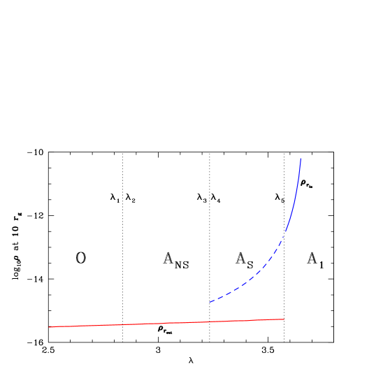
Figure 3: In the figure, $\rho_{r_{out}}$ and $\rho_{r_{in}}$ represent the density of the accreting material measured at 10$r_{g}$ along the transonic accretion passing through the outer and the inner sonic points, respectively. The long dashed line corresponds to the range of the angular momentum for which a steady standing Rankine Hugoniot shock forms. The figure has been drawn for $\left[{\cal E}=1.0000033,\gamma=4/3,a=0.3\right]$.

6 Continuity in the parameter space and the hysteresis effect

The heteroclinic fish like solution as described in the section 5.6 marks the transition between two different flow topologies, a multi-transonic accretion with a built-in homoclinic orbit (as shown in the successive panel figures (ii) - (iv)) and a mono-transonic accretion with an additional non accessible homoclinic orbit (as shown in the panel figure (iv)). It is to be understood that the solutions with shock for the value of the flow angular momentum higher than $\lambda_{5}$ are of completely different character compared to the solution parametrized by the value of angular momentum lower than $\lambda_{5}$. We illustrate this issue through the following procedure:

We set $r_{10}=10r_{g}$ as our reference point. For a transonic solution, we then calculate the density of the accerting matter at $r_{10}$ as a function of $\lambda$, keeping the other initial boundary conditions $\left[{\cal E},\gamma,a\right]$ fixed. This has to be done in several steps. For mono-transonic accretion passing through the outer sonic point only, we can have only one choice to calculate $\rho$ at $r_{10}$, that is to calculate the density at $r_{10}$ only on the solution passing through the outer sonic point, $r_{out}$, and denoting it by $\rho_{r_{out}}$. We do it without any ambiguity for a span of value of $\lambda$, starting from a very small value (almost equal to zero, just when the departure from the pure Bondi type accretion stars) upto the value $\lambda=\lambda_{1}$. Beyond $\lambda_{1}$, for $\lambda>\lambda_{1}$, in principle there are two choices for the density calculation at $r_{10}$. One is along the flow passing through $r_{out}$, to obtain $\rho_{r_{out}}$ for the multi-transonic flow. Another option is to compute the density $\rho_{r_{in}}$ along the multi-transonic accretion flow passing through the inner sonic point $r_{in}$. Both $\rho_{r_{out}}$ and $\rho_{r_{in}}$ can be calculated as a function of $\lambda$ for the span $\lambda_{1}<\lambda<\lambda_{5}$. However, since for the span $\lambda_{1}<\lambda<\lambda_{3}$ shock does not form, $\rho_{r_{in}}$ is a meaningless quantity to define for this span of $\lambda$, and thus for any value of the angular momentum upto $\lambda=\lambda_{3}$, density at $r_{10}$ means $\rho_{r_{out}}$ only. However, the situation is different for $\lambda_{3}<\lambda{\leq}\lambda_{5}$, where both $\rho_{r_{out}}$ and $\rho_{r_{in}}$ can have feasible meaning. However, $\rho_{r_{out}}$ is practically meaningful if shock does not form (since it has been thoroughly verified that the lowest possible shock location $r^{\sf minimum}_{\sf sh}$ for the entire range of our choice of $\left[{\cal E},\lambda,\gamma,a\right]$ is always greater than $r_{10}$), and $\rho_{r_{in}}$ is practically meaningful only if the shock forms. Beyond $\lambda_{5}$, for $\lambda>\lambda_{5}$, once again one has mono-transonic accretion (with an additional homoclinic orbit of course), now passing through the inner sonic point $r_{in}$. Hence the measured density at $r_{10}$ for $\lambda>\lambda_{5}$ implies $\rho_{r_{in}}$ only.

Hence, we have $\rho_{r_{out}}$ defined over the range for any value of the flow angular momentum upto $\lambda=\lambda_{5}$, and, on the contrary, $\rho_{r_{in}}$ is defined only over the range $\lambda{\geq}\lambda_{3}$. In figure 3, we plot, in logarithmic scale, $\rho_{r_{out}}$ using the solid line (red coloured in the online edition) and $\rho_{r_{in}}$ using the solid line (in the region IV) and the dashed line (in the region III) respectively, as a function of the specific flow angular momentum $\lambda$.

The local density changes by a factor over 500 at $\lambda_{5}$ which well illustrates the global quantitative change in the flow. However, when we add the solutions passing through the inner and the outer sonic points with a shock to the same plot, those solutions form a continuation of the previous branch below $\lambda_{5}$. The shock for $\lambda$ just below $\lambda_{5}$ is extremely weak (with the corresponding shock strength having value very close to the unity), and located infinitesimally close inward of the outer critical point. With a further decrease of $\lambda$ the shock strength measured as a ratio of the Mach numbers above and below the shock increases monotonically, and the shock position moves inward.

The branch with a shock also does not cover the whole range of angular momentum values – there is a minimum value of $\lambda$ (for a given Bernoulli constant, the polytropic index and the black hole spin) for which the Rankine-Hugoniot conditions (see Sect. 5.5) can be satisfied. This value, marked as $\lambda_{4}$ in the section 5.7, describes the discontinuous change in the solution along the branch with a shock with a further drop in the angular momentum, as for still lower values of $\lambda$ only the solutions without shock exist. The local density change in the flow at $r_{10}$ accompanying the slight change of angular momentum along this branch is by a factor 4, much less than the factor 500 at the transition at $\lambda_{5}$ for the shock-free solutions.

Since the system is likely to choose a solution close to the previous one under the slight change of the outer boundary conditions (here, the angular momentum), the choice between the solution with a shock and without a shock for $\lambda_{4}<\lambda<\lambda_{5}$ will depend on the previous history of the system. If the initial value of the angular momentum is lower than $\lambda_{4}$ and slowly increases the system will follow the lower branch ($\rho_{r_{out}}$) in Fig. 3 without a shock and will show a dramatic change when passing from $\lambda<\lambda_{5}$ to $\lambda>\lambda_{5}$. If, on the other hand, the system evolution starts with $\lambda>\lambda_{5}$ and the angular momentum of the infalling material slowly decreases the system is more likely to follow the upper branch in Fig. 3, without any discontinuity in the appearance down to $\lambda_{4}$ but the solution will display an increasingly stronger shock with a quasi-stationary increase of the angular momentum of the matter.

We thus expect a hysteresis effect in the system behavior under the conditions of slowly varying initial angular momentum of the accreting matter. This may in turn lead to some asymmetry in the lightcurves of the systems accreting in such a mode. The local density at $10r_{g}$ is an indicator of the system luminosity (the synchrotron emission increases with the plasma density and magnetic field). The increase in the local density indicates an increase in a source brightness. Since the discontinuity in the density profile is larger when the angular momentum and consequently the density increases (at $\lambda_{5}$) the brightening should be faster/stronger than the subsequent faintenning of the source (evolution along the upper branch ($\rho_{r_{in}}$) in Fig. 3, down to $\lambda_{4}$). However, detailed study of this effect and comparison with observational data is beyond the scope of the present paper.

In this context, it is to be noted here that the shock strength, which correlates with the entropy enhancement ratio ${R_{\dot{\Xi}}}$ at the shock, monotonically increases with decreasing $\lambda$, and at the same time anti-correlates with the shock location itself. The variation of the shock strength (solid line marked by $M_{-}/M_{+}$) and ${R_{\dot{\Xi}}}$ (dotted line marked by ${R_{\dot{\Xi}}}$) with $\lambda$ is shown in the figure 4. The strongest shock thus forms closer to the black hole. From observational data, it is expected that the QPO profile of the SgrA* black hole corresponding to a small length scale shock formation. Shocks formed for the angular momentum $\lambda{\sim}\lambda_{4}$ thus, might corresponds to such QPO behaviour.

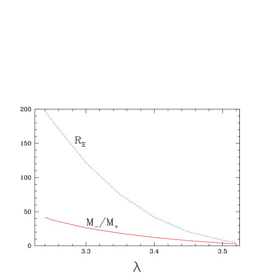
Figure 4: The variation of the shock strength (solid line, red coloured in the online version) and the entropy accration rate ratio at the shock (dotted line, blue coloured in the online version) as a function of the flow angular momentum for a fixed set of initial boundary conditions $\left[{\cal E}=1.0000033,\gamma=4/3,a=0.3\right]$ Shock strength anti-correlates with the shock location. As a result, shocks formed closer to the black hole are stronger.

7 A Lyapunov like treatment

As we already have observed, for an extended region of the parameter space describing the multi-transonic accretion flow, shock does not form in spite of the the availability of two saddle type sonic points to the accretion flow to pass through. This region has been marked as ${\rm A_{\rm NS}}$, and is bounded by the span of the specific angular momentum $\left[\lambda_{2}-\lambda_{3}\right]$. One might raise the question about what dictates the flow not to make a shock transition even if the shocked flow can have the saddle type inner sonic point available to pass through. In other words, given all the favourable conditions, i.e., the presence of two real physical sonic points, and a larger than one entropy accretion rate ratio for the flows passing through these sonic points (with higher entropy accretion rate for the flow passing thorough the outer sonic point), what prohibits the Rankine Hugoniot condition to be satisfied, as it gets satisfied for the region ${\rm A_{\rm S}}$? In reality, no information can readily be obtained from the initial boundary conditions $\left[{\cal E},\lambda,\gamma,a\right]$ as well as the measure of the entropy accretion rate (which, of course, is purely a function of $\left[{\cal E},\lambda,\gamma,a\right]$, and hence, does not impose any additional condition) which may provide some certain well defined conditions predicting about the validity of the Rankine Hugoniot conditions over certain region of the parameter space describing the multi-transonic accretion flow.

Usual trends in the contemporary literature ((Chakrabarti, 1989; Das, 2002) and references therein) to explain the origin and the characteristic features of the ${\rm A_{\rm NS}}$ region is to make hypothesis that the shock may become oscillatory in that region, in absence of the fine tuning condition of the entropy generation at the shock (that the difference between the entropy accretion rate should exactly be equal to the excess amount of ${\dot{\Xi}}$ produced at the shock), and the region ${\rm A_{\rm NS}}$ thus has been attributed to explain, in analogy with the results obtained from the full numerical time dependent simulation of the shocked axisymmetric flow (see, e.g., (Sponholz & Molteni, 1994; Okuda et al., 2007) and references therein), the formation of the quasi-periodic oscillation of the black hole candidates. This approach, however, is fundamentally inconsistent from the mathematical perspective. The parameter space corresponding to the formation of the ${\rm A_{\rm NS}}$ region (of any region of the parameter space shown in the figure 1) is obtained from a completely stationary configuration, where the mother equations have been constructed as a set of explicit time independent equations. The notion of the oscillation of the shock (or the very phrase ’‘oscillation’ itself) is associated with the dynamical temporal evolution of the configuration governed by a set of full time dependent equations. Hence, although for full time dependent numerical simulations, the appearance of the shock oscillation can be considered as a consistent physical scenario, such shock oscillation prescriptions can never be applied to clarify any results which has been obtained by solving a set of explicit steady state equations.

The above issue prompted us to put forward a theoretical condition, which, within the framework of the stationary configuration, will be able to explain why the entire region of the multi-transonic accretion parameter space will not allow a stationary shock solution, and, instead, only a restricted part of the region will produce a shocked accretion flow. We propose a Lyapunov like treatment of the transonic accretion solution, within a complete stationary framework, to accomplish the above task. It is not quite uncommon in the literature to reply on a Lyapunov like treatment, within the configuration of a stationary set up which contains an equilibrium point (the critical point) to study the state transition of such systems, subjected to a small variation of the overall parameter space. Such a methodology have been applied to several systems, for example, to describe the state transition of a spin galas phase in terms of the $T=0$ critical point where $T$ is the absolute temperature ((Bray & Moore, 1987)), or to study the thermodynamic stability of the protein like heteropolymers against the biological mutation process, by considering such process as a perturbation ((Bussemaker et al., 1997)). In what follows, we propose a one dimensional effective Lyapunov index ${\sf L_{\sf eff}}$. ${\sf L_{\sf eff}}$ will exclusively predict which final state – a shocked flow passing through both the outer and the inner sonic points, or a shock free flow passing only through the outer sonic point – a multi-transonic accretion will follow, subjected to the specific initial boundary conditions, and the infinitesimal variation of the control parameter describing the secular evolution of the flow.

Proposition 7.1

On a two dimensional parameter space spanned by $\left[{\cal E},\lambda\right]$ as shown in the figure 1. let us consider two transonic solutions characterized by infinitesimally different values of the specific flow angular momentum $\lambda_{i}$ and $\lambda_{f}$, satisfying the condition

$${\sf Lt}_{{\epsilon}{\rightarrow}0}~{}{|}\lambda_{i}-\lambda_{f}{|}{=}{\epsilon}$$ (56)

Let $u_{1}(r)$ and $u_{2}(r)$ be the values of the advective velocity at a certain value of the radial distance $r$ for two transonic solutions characterized by very close values of the angular momentum $\lambda_{1}$ and $\lambda_{2}$ respectively, with ${\cal E}$ and $\gamma$ kept fixed. Let $u_{1}(r-R)$ and $u_{2}(r-R)$ be the corresponding velocities for the above-mentioned transonic flow solutions at the radial distance $r-R$, with the obvious requirement that $R<r$. We then define the effective Lyapunov exponent ${\sf L_{\sf eff}}$, so that the following condition holds:

$$\frac{u_{1}(r-R)-u_{2}(r-R)}{u_{1}(r)-u_{2}(r)}\sim e^{{\sf L_{\sf eff}}R}.$$ (57)

The effective index ${\sf L_{\sf eff}}$ can also be calculated by varying ${\cal E}$ instead of $\lambda$.

Without any loss of generality, one can normalize the constant to appear in front of the $e^{{\sf L_{\sf eff}}R}$ and can define the effective Lyapunov exponent as:

$${{\sf L_{\sf eff}}}=\frac{1}{R}\left\{\frac{u_{1}(r-R)-u_{2}(r-R)}{u_{1}(r)-u_{2}(r)}\right\}$$ (58)

It is obvious from the expression of ${{\sf L_{\sf eff}}}$ that for accretion, the effective Lyapunov index is a measure of how drastically the output (Mach number variation in the flow topology) will change with respect to an arbitrary small perturbation in the control parameter (the specific angular momentum $\lambda$, for our case). Hence there is no harm in assuming that ${{\sf L_{\sf eff}}}$ does share the properties of a Lyapunov exponent in the context that a higher value of the modulus of ${{\sf L_{\sf eff}}}$ indicates a greater available volume of the phase space (in connection to the Kaplan-Yorke conjecture (Kaplan & Yorke, 1979)).

We now consider two different values of angular momentum infinitesimally separated and lying at two different side of the value $\lambda=\lambda_{1}$ (the value of the angular momentum corresponding to the boundary of the O and the A region of the parameter space diagram as shown in the figure 1), as $\lambda_{\pm}$ where $\lambda_{-}=\lambda_{1}-\epsilon$ and $\lambda_{+}=\lambda_{1}+\epsilon$ for $\epsilon{\rightarrow}0$. For $\lambda=\lambda_{-}$, one has a mono-transonic accretion only through the outer sonic point, and $\lambda=\lambda_{+}$ provides the multi-critical accretion. We now calculate the ${{\sf L_{\sf eff}}}$ for $\left[r=10r_{g},R=0.2r_{g},\lambda_{-}=2.839,\lambda_{+}=2.84\right]$, where $u_{1}$ corresponds to the solution characterized by $\lambda_{-}$ and $u_{2}$ corresponds to the solution characterized by $\lambda=\lambda_{2}$, all for the initial boundary condition $\left[{\cal E}=1.0000033,\gamma=\frac{4}{3},a=0.3\right]$ for the following two different situations as described below:

1. For $\lambda=\lambda_{+}$, we fist assume that the accretion flow, even formally being multi-transonic, passes only through the outer sonic point (which is the reality because solution characterized by $\lambda_{+}$ is a shock free solution from ${\rm A}_{\rm NS}$). We then calculate $u_{2}(r)$ and $u_{2}(r-R)$ for flow passing through the outer sonic point. For such situation, we denote the effective Lyapunov index as ${{\sf L_{\sf eff}}}^{\left[\lambda_{-}^{\rm out},\lambda_{+}^{\rm out}\right]}$, where it is understood that the mono-transonic accretion characterized by $\lambda_{-}$ passes only through the outer sonic point and the the effective Lyapunov index is being calculated at $r=10r_{g}$ for accretion solution characterized by $\lambda_{+}$, which has been considered to pass through the outer sonic point, where the outer sonic point is larger than $r=10r_{g}$. Within the bracket, $\lambda_{-}^{\rm out}$ has been written first, and then $\lambda_{+}^{\rm out}$. This sequence indicates that the change of the specific angular momentum has been made such a was that a transition is being induced from the mono-transonic accretion (passing through the outer sonic point) characterized by $\lambda_{-}$ to the multi-transonic accretion (but here again, passing only through the corresponding outer sonic point, and does not encounter the inner sonic point because shock does not form in this case) characterized by $\lambda_{+}$. The modulus of the numerical value of the effective Lyapunov index, which has been denoted by ${\sf mod}\left({{\sf L_{\sf eff}}}^{\left[\lambda_{-}^{\rm out},\lambda_{+}^{\rm out}\right]}\right)$, is found to be $\sim{1.6631}$ for the present situation.

2. Here for $\lambda_{+}$, we assume, for a hypothetical situation, what would have been the value of the effective Lyapunov index at $r=10r_{g}$, if, for whatever reason, the muli-critical accretion would finally pass through the inner sonic point. Hence $u_{2}(r)$ and $u_{2}(r-R)$ have been calculated for flow passing through the inner sonic point, and the corresponding effective Lyapunov index ${{\sf L_{\sf eff}}}^{\left[\lambda_{-}^{\rm out},\lambda_{+}^{\rm in}\right]}$ has been computed. The the corresponding modulus of the numerical value of ${{\sf L_{\sf eff}}}^{\left[\lambda_{-}^{\rm out},\lambda_{+}^{\rm out}\right]}$, which is denoted as ${\sf mod}\left({{\sf L_{\sf eff}}}^{\left[\lambda_{-}^{\rm out},\lambda_{+}^{\rm in}\right]}\right)$ is found to be ${\sim}1.60738$.

We thus clearly have

$${\sf mod}\left({{\sf L_{\sf eff}}}^{\left[\lambda_{-}^{\rm out},\lambda_{+}^{\rm out}\right]}\right)>{\sf mod}\left({{\sf L_{\sf eff}}}^{\left[\lambda_{-}^{\rm out},\lambda_{+}^{\rm in}\right]}\right)$$ (59)

We now apprehend what does the above inequality indicate.

If one makes a transition from the mono-transonic flow to the multi-transonic flow by an incremental smooth change of the specific angular momentum, ${{\sf L_{\sf eff}}}$ is a essentially a measure of the probability of the outcome of final state corresponding to such a transition. The effective Lyapunov exponent has been defined in such a way that the above findings allows us to make the following statement:

Conjecture 7.2

For a certain transonic accretion state characterized by a control parameter $c_{i}$ ($c_{i}=\lambda_{-}=\lambda_{1}-\epsilon$ for the present purpose), if there are two possible transitions to two different transonic states, both characterized by the same value of the final control parameter $c_{f}$ ($c_{f}=\lambda_{+}=\lambda_{1}+\epsilon$ for the present purpose), differing from $c_{i}$ by an infinitesimal measure $\epsilon{\rightarrow}0$, and if such transitions can be quantified by two different effective Lyapunov indices ${{\sf L^{1}_{\sf eff}}}$ and ${{\sf L^{2}_{\sf eff}}}$, then the transition characterized by the higher absolute value (the modulus of the numerical value) of the effective Lyapunov index is a more probable outcome with greater likelihood, since a higher value of the Lyapunov index indicates a greater available occupancy of the phase volume for the solution.

This means that according to the inequality (59), the probability of finding (at $r=10r_{g}$) the accretion flow passing through the outer sonic point (shock free multi-criticality) is higher than the probability of finding it to pass through the inner sonic point (shocked multi-transonic accretion). And that is exactly what is observed for the ${\sf A_{\sf NS}}$ region. We calculate, for a wide range of $r$ and $R$, with $r$ lying close to the inner sonic point, that is, closer to the black hole in comparison to any ‘anticipated’ artificial shock location, so as to calculate the ${{\sf L_{\sf eff}}}$ for an ‘artificial’ post shock flow (had it been the case that the shock would, at all, form, which clearly does not, in reality). This procedure guarantees the consistency of checking the probability of two possible outcomes at a length scale where one can distinguish a shocked and a shock free solution. For all possible configurations, we consistently found that the inequality (59) always holds good.

What about the true multi-transonic accretion flow structure allowing a standing shock? We can show that sufficient room for such flow configuration is available as well. For this purpose, consider two infinitesimally separated value of $\lambda$, $\lambda_{\pm}$ at the opposite sides of the boundary separating the ${\sf A}$ and the ${\sf A_{1}}$ region. Here $\lambda_{-}=\lambda_{5}-\epsilon$ provides a multi-transonic accretion and $\lambda_{+}=\lambda_{5}+\epsilon$ provides a transonic accretion passing only through the inner sonic point (and associated with a homoclinic orbit characterized by an additional pair of critical point, none of which a real physical accretion solution can pas through). We now calculate the corresponding effective Lyapunov indices for a decremental smooth change of the angular momentum. The unique initial state (accretion passing only through the inner sonic point) is characterized by $\lambda_{+}$. Two final states, both characterized by $\lambda_{-}$, are available. The first option for such final state is a hypothetical shock free multi-critical accretion passing through the outer sonic point only, on which $u_{2}(r)$ and $u_{2}(r-R)$ are measured at some specified value of $r$ and $R$. The corresponding effective Lyapunov index being ${{\sf L_{\sf eff}}}^{\left[\lambda_{+}^{\rm in},\lambda_{-}^{\rm out}\right]}$. For the other variant (the actual case), the shock forms and the accretion finally passes through the inner sonic point. The corresponding index is ${{\sf L_{\sf eff}}}^{\left[\lambda_{+}^{\rm in},\lambda_{-}^{\rm in}\right]}$.

A suitable choice of $r$ is trivial, it has to be smaller than the smallest possible shock location for $\lambda_{-}$ type flow, so as to the length scale for our interest lies in the post-shock region. All possible variation of such $r$ and $R$ confirms the generic nature of the following inequality

$${\sf mod}\left({{\sf L_{\sf eff}}}^{\left[\lambda_{+}^{\rm in},\lambda_{-}^{\rm in}\right]}\right)>{\sf mod}\left({{\sf L-{\sf eff}}}^{\left[\lambda_{+}^{\rm in},\lambda_{+}^{\rm out}\right]}\right)$$ (60)

Lemma 7.3

For an incremental smooth change of the flow specific angular momentum, a transition from a mono-critical mono-transonic flow to a multi-critical flow will not produce a shock, however, for a decremental smooth change of $\lambda$, a transition from a mono-transonic accretion to a multi-critical accretion must accompany a standing shock, and the multi-critical accretion is a true multi-transonic one.

It is interesting to note that the above lemma has one to one correspondence with our findings related to the hysteresis effect as described in the previous section.

We thus define an independent quantity, within a framework of a purely stationary configuration, namely the effective Lyapunov index ${{\sf L_{\sf eff}}}$, which, for the first time in literature, can analytically explain why one obtains shock free solutions even for a multi-critical flow configuration.

8 Discussion

In the present paper we study the topology of the low angular momentum flow onto a black hole as a function of the flow global parameters. Such a study may indicate the behaviour of the time evolution of the flow seen as a sequence of quasi-stationary stages.

For a given set of other parameters (the Bernoulli constant, adiabatic index and the Kerr parameter) the change in the angular momentum of the flow (determined by the outer boundary conditions) leads to a sequence of solutions passing through two discontinuous changes in the flow topology, and consequently, in the flow local parameters.

The discontinuity at $\lambda_{5}$ corresponds to a heteroclinic solution (a ‘fish’ topology) with a flow line connecting the inner and the outer critical points. As we argue in Sect. 6, the physical flow is likely to change discontinuously at $\lambda_{5}$ if the angular momentum increases from $\lambda<\lambda_{5}$ to $\lambda>\lambda_{5}$ as a result of systematic secular evolution, and then solutions both for $\lambda<\lambda_{5}$ and $\lambda<\lambda_{5}$ do not develop a shock. However, if in the course of secular evolution the angular momentum decreases from $\lambda>\lambda_{5}$ to $\lambda<\lambda_{5}$ the systems evolves through $\lambda_{5}$ without showing any discontinuous change but instead develops a shock, with the strength of the shock increasing with the $\lambda_{5}/\lambda$ ratio.

The above mentioned finding has further been supported by a Lyapunov like treatment of the state transition of the flow, as discussed in detail in Sect. 7.

The discontinuity at $\lambda_{4}$ corresponds to the minimum value of the angular momentum for which the solutions with shocks exist. It is likely to show up if the angular momentum systematically decreases, first from $\lambda>\lambda_{5}$ to $\lambda<\lambda_{5}$ (following the branch with shocks) and then down below $\lambda<\lambda_{4}$. The solution must then change discontinuously to the one without a shock. The reverse evolution does not lead to discontinuity as the flow then proceeds as a shock-free solution continuously up to $\lambda_{5}$ where it reaches the critical ‘fish’ topology.

The analytical study of the solution stability close to ‘fish ’ topology ($\lambda\propto\lambda_{5}$) cannot be performed since infinitesimal changes in the solution parameters lead to the arbitrarily large change in the flow parameters. The problem should be addressed through time-dependent dynamical simulations.

The issue of the topological change in the flow is generic and not related to any specific choice of the other flow parameters. We will show in our next work (Das & Czerny, in preparation) that the ‘fish’ topology always appears as a boundary between the inflow through the inner critical point and through the outer critical point, irrespective of the flow geometry (as long as it contains some non zero angular momentum), the specific metric, and the choice of the equation of state.

Our discussion shows that both solutions with, and without a shock, are likely to be met in real sources accreting material with low angular momentum, and the actual choice of the solution by the system depends on the flow history.

If the accretion parameters in an astrophysical system are in the range somewhat broader than $\lambda_{4}$ - $\lambda_{5}$ and vary in time the system will show sudden rapid changes in the luminosity accompanying the sudden flow restucturization. We qualitatively predict the appearance of flares with more rapid increase of the luminosity (when crossing from $\lambda<\lambda_{5}$ to $\lambda>\lambda_{5}$) followed by a slow decay (evolution partially along the shock branch down to $\lambda<\lambda_{4}$). Quantitative estimates would require computations of the flow emissivity.

The appearance of the homoclinic orbit on the phase portrait is not unique for the axisymmetric rotating flows only. For spherically symmetric accretion with self gravity and radiative processes incorporated into it Karkowski, Malec & Roszkowski (2008); Karkowski, Malec, Roszkowski & Swierczynski (2009), such homoclinic paths would also appear Rembiasz (2009), making the spherically symmetric accretion to be a bi-critical flow. It appears that the emergence of a homoclinic orbit is due to the smooth decrement of the radial inflow velocity, due to the centrifugally supported barrier for rotating flow, while due to the radiative losses for the spherical accretion.

In this work, we have used a relatively lower value of the Kerr parameter ($a=0.3$) as a representative one. This does not, by any means, limit the applicability of our methodology for the case of black holes possessing higher value of the spin angular momentum because the Kerr parameter has been treated as a free parameter in our construction and any value of $a$ can easily be plugged in into our model set up. For example, we obtain consistent shock location for the value of $a$ as high as $0.99$ (ad for values of $\gamma$ other than 4/3) as well. We can, compute the shock location and all other shock related quantities in general as a function of the Kerr parameter as well, and that has been presented in some other work (Barai et al. in preparation).

Some of the results presented in this paper may also apply to GRB. In this event, modeled as a failed supernova, the star first collapses due to the fuel exhaustion, the collapse is halted close to the core (at $\sim 500$km) and replaced by expansion. Part of the stellar envelope is rejected but the neutrino cooling stops part of the material and subsequently the slow fallback stage takes place MacFadyen, Woosley & Heger (2001) onto a newly formed compact object. This accretion stage of the long gamma-ray burst can be described within the frame of our model assuming that the angular momentum of the back falling envelope is not large. If the accretion flow proceeds through a solution with a shock, the shock-related periodic oscillations may in a natural way explain for example the fast optical variability of the Naked-Eye burst GRB080319B Beskin et al. (2009).

References

- Anderson (1989) Anderson, M. 1989, MNRAS, 239, 19
- Abraham et al. (2006) Abraham, H., Bilić, N., Das, T. K., 2006, Classical and Quantum Gravity, 23, 2371
- Abramowicz et al. (1988) Abramowicz, M. A., Czerny, B., Lasota, J. P., Szuszkiewicz, E., 1988, ApJ, 332, 646
- Abramowicz & Chakrabarti (1990) Abramowicz, M. A., & Chakrabarti, S. K., 1990, ApJ, 350, 281
- Abramowicz, Lanza & Pervival (1997) Abramowicz, M. A., Lanza, A., & Percival, M. J. 1997, ApJ, 479, 179
- Abramowicz & Kato (1989) Abramowicz, M. A., Kato, S. 1989, ApJ, 336, 304
- Abramowicz & Zurek (1981) Abramowicz, M. A., Zurek, W. H. 1981, ApJ, 246, 314
- Afshordi & Paczyński (2003) Afshordi, N., Paczyński, B., 2003, ApJ, 592, 354
- Artemova et al. (1996) Artemova, I. V., Björnsson, G., Novikov, I. D., 1996, ApJ, 461, 565
- Armitage, Reynolds & Chiang (2001) Armitage, P. J., Reynolds, C. S., & Chiang, J., 2001, APJ, 648, 868.
- Barai et al. (2004) Barai, P., Das, T. K., Wiita, P. J., 2004, ApJ, 613, L49
- Beloborodov & Illarionov (1991) Beloborodov, A. M., & Illarionov, A. F. 1991, MNRAS, 323, 167
- Beskin et al. (2009) Beskin, G., Karpov, S., Bondar, S., Guarnieri, A., Bartolini, C., Greco, G., & Piccioni, A., 2009, arXiv:0905.4431v1 [astro-ph.HE]
- Bhattacharjee & Ray (2007) Bhattacharjee, J. K., Ray, A. K., 2007, ApJ, 668, 409
- Bhattacharjee et al. (2009) Bhattacharjee, J. K., Bhattacharya, A., Das, T. K., & Ray, A. K., 2009, to appear in MNRAS, see also arXiv:0812.4793v1 [astro-ph].
- Bisikalo et al. (1998) Bisikalo, A. A., Boyarchuk, V. M., Chechetkin, V. M., Kuznetsov, O. A., & Molteni, D. 1998, MNRAS, 300, 39
- Bondi (1952) Bondi, H. 1952, MNRAS, 112, 195
- Boyer & Lindquist (1967) Boyer, R. H., & Lindquist, R. W. 1967, J. Math. Phys. 8, 265
- Bray & Moore (1987) Bray, A. J., & Moore, M. A. 1987, Phys. rev. Lett. 58, 57
- Bussemaker et al. (1997) Bussemaker, H. J., Thirumalai, D., & Bhattacharjee, J. K., 1997, Physical Review Letters, Volume 79, Issue 18, November 3, 1997, pp.3530-3533
- Caditz & Tsuruta (1998) Caditz, D. M., & Tsuruta, S. 1998, ApJ, 501, 242
- Chakrabarti (1989) Chakrabarti, S. K., 1989, ApJ, 347, 365
- Chakrabarti (1990) Chakrabarti, S. K., 1990, Theory of Transonic Astrophysical Flows, World Scientific, Singapore
- Chakrabarti & Titarchuk (1995) Chakrabarti, S. K., Titarchuk, L. G., 1995, ApJ, 455, 623
- Chattopadhyay & Das (2007) Chattopadhyay, I., & Das, S., 2007, New Astronomy, Volume 12, Issue 6, p. 454
- Chaudhury et al. (2006) Chaudhury, S., Ray, A. K., Das, T. K., 2006, MNRAS, 373, 146
- Chen et al. (1997) Chen, X., Abramowicz, M. A., Lasota, J. P., 1993, ApJ, 476, 61
- Chen & Taam (1993) Chen, X., Taam, R., 1993, ApJ, 412, 254
- Chicone (2006) Chicone, C., 2006, ‘Ordinary Differential Equations with Applications’, Springer; 2nd edition.
- Das (2007) Das, S., 2007, MNRAS, 376, 1659
- Das & Chattopadhyay (2007) Das, S., & Chattopadhyay, I., 2008, New Astronomy, Volume 13, Issue 8, p. 549
- Das & Chakrabarti (1999) Das, T. K., & Chakrabarti, S. K. 1999, Class. Quantum Grav. 16, 3879
- Das (2002) Das, T. K., 2002, ApJ, 577, 880
- Das et al. (2003) Das, T. K., Pendharkar, J. K., Mitra, S., 2003, ApJ, 592, 1078
- Das, Rao & Vadawale (2003) Das, T. K., Rao, A. R., & Vadawale, S. R. 2003, MNRAS, 343, 443
- Ferrari et al. (1985) Ferrari, A., Trussoni, E., Rosner, R., and Tsinganos, K. 1985, ApJ, 294, 397
- Frank et al. (2002) Frank, J., King, A., Raine, D., 2002, Accretion Power in Astrophysics, Cambridge University Press, Cambridge
- Fukue (1983) Fukue, J., 1983, PASJ, 35, 355
- Fukue (1987) Fukue, J., 1987, PASJ, 39, 309
- Fukue (2004) Fukue, J., 2004, PASJ, 56, 681
- Fukue (2004a) Fukue, J., 2004, PASJ, 56, 959
- Fukumura & Kazanas (2007) Fukumura, K., Kazanas, D., 2007, ApJ, 669, 85
- Fukumura & Tsuruta (2004) Fukumura, K., & Tsuruta, S., 2004, ApJ, 611, 964
- Goswami et al. (2007) Goswami, S., Khan, S. N., Ray, A. K., Das, T. K., 2007, MNRAS, 378, 1407
- Hawley & Krolik (2001) Hawley, J. F., & Krolik, J. H., 2001, APJ, 548, 348
- Ho (1999) Ho, L. C. 1999, in Observational Evidence For Black Holes in the Universe, ed. S. K. Chakrabarti (Dordrecht: Kluwer), 153
- Igumenshchev & Abramowicz (1999) Igumenshchev, I. V. & Abramowicz, M. A. 1999, MNRAS, 303, 309
- Igumenshchev & Beloborodov (1997) Igumenshchev, I. V., & Beloborodov, A. M., 1997, MNRAS, 284, 767
- Illarionov & Sunyaev (1975) Illarionov, A.F., & Sunyaev, R. A. 1975a, A & A, 39, 205
- Illarionov (1988) Illarionov, A. F. 1988, Soviet Astron., 31, 618
- Jordan & Smith (1999) Jordan, D. W., Smith, P., 1999, Nonlinear Ordinary Differential Equations, Oxford University Press, Oxford
- Kafatos & Yang (1994) Kafatos, M., Yang, R. X., 1994, MNRAS, 268, 925
- Kaplan & Yorke (1979) Kaplan, J. L., & Yorke, J. A., 1979, in Chaotic Behaviour of Multidimensional Difference Equations, Lecture Notes in Mathematics, eds. Peitgen, H.-O., & Walther, H.-O., (Springer, Berlin), Vol. 730, pp. 204-227.
- Karkowski, Malec & Roszkowski (2008) Karkowski, J., Malec, E., & Roszkowski, K., 2008, A & A, Volume 479, Issue 1, pp.161-166
- Karkowski, Malec, Roszkowski & Swierczynski (2009) Karkowski, J., Malec, E., Roszkowski, K., & Swierczynski, Z., 2009, Acta Physica Polonica B, Vol. 40, No 2, pp. 273.
- Kato (1978) Kato, S., 1978, MNRAS, 185, 629
- Kato et al. (198yy8) Kato, S., Honma, F., Matsumoto, R., 1988, MNRAS, 231, 37
- Kato, Fukue & Mineshige (1998) Kato, S., Fukue, J., & Mineshige, S., 1998, Black Hole Accretion Disc, Kyoto University Press.
- Landau & Lifshitz (1987) Landau, L. D., Lifshitz, E. M., 1987, Fluid Mechanics, Butterworth-Heinemann, Oxford
- Lanzafame (2008) Lanzafame, G., 2008, ASPC, 385, 115
- Liang & Thompson (1980) Liang, E. P. T., Thomson, K. A., 1980, ApJ, 240, 271
- Liang & Nolan (1980) Liang, E. P. T., & Nolan, P. L., 1984, Space. Sci. Rev. 38, 353
- Lu (1985) Lu, J. F. 1985, A & A, 148, 176
- Lu (1986) Lu, J. F. 1986, Gen. Rel. Grav. 18, 45L
- Lu et al. (1997) Lu, J. F., Yu, K. N., Yuan, F., Young, E. C. M., 1997, A & A, 321, 665
- Lu & Gu (2004) Lu, J. F., & Gu, W. M., 2004, Chin. Phys. Lett., 21, 2551
- MacFadyen, Woosley & Heger (2001) MacFadyen, A. I., Woosley, S. E., & Heger, A., 2001, The Astrophysical Journal, Volume 550, Issue 1, pp. 410-425
- Manmoto (2000) Manmoto, T. 2000, ApJ, 534, 734
- Matsumoto et al. (1984) Matsumoto, R., Kato, S., Fukue, J., Okazaki, A. T., 1984, PASJ, 36, 71
- Moscibrodzka, Das & Czerny (2006) Moscibrodzka, M., Das, T. K., & Czerny, B. 2006, MNRAS, 370, 219
- Muchotrzeb & Paczyński (1982) Muchotrzeb, B., & Paczynski, B., 1982, Acta Actron. 32, 1
- Muchotrzeb (1983) Muchotrzeb, B., 1983, Acta Astron. 33, 79
- Muchotrzeb-Czerny (1986) Muchotrzeb-Czerny, B., 1986, Acta Astronomica, 36, 1
- Mukhopadhyay (1999) Mukhopadhyay, B., 1999, Indian J. Phys., Part B, Vol. 73B, No. 6, p. 917
- Nagakura & Yamada (2008) Nagakura, H., Yamada, S., 2008, ApJ, 689, 391
- Nagakura & Yamada (2009) Nagakura, H., Yamada, S., 2009, ApJ, 696,2026
- Nakayama & Fukue (1989) Nakayama, K., Fukue, J., 1989, PASJ, 41, 271
- Nakayama (1996) Nakayama, K., 1996, MNRAS, 281, 226
- Narayan, Kato & Honma (1997) Narayan, R., Kato, S., & Honma, F., 1997, APJ, 476, 49
- Novikov & Thorne (1973) Novikov, I., & Thorne, K. S. 1973, in Black Holes,eds. c. De Witt and B. De Witt(Gordon and Breach, New York).
- Okuda et al. (2004) Okuda, T., Teresi, V., Toscano, E., & Molteni, D., 2004, Publications of the Astronomical Society of Japan, Vol.56, No.3, pp. 547-552
- Okuda et al. (2007) Okuda, T., Teresi, V., & Molteni, D., 2007, MNRAS, 377, 1431
- Paczyński (1987) Paczyński, B., 1987, Nature, 327, 303
- Paczyński & Wiita (1980) Paczyński, B., Wiita P. J., 1980, A&A, 88, 23
- Pariev (1996) Pariev, V. I., 1996, MNRAS, 283, 1264
- Parker (1965) Parker, E. N., 1965, Space Science Reviews, vol. 4, p.666
- Peitz & Appl (1997) Peitz, J., Appl, S., 1997, MNRAS, 286, 681
- Pringle (1981) Pringle, J. E., 1981, ARA&A, 19, 137
- Proga & Begelman (2003) Proga, D., & Begelman, M. C., 2003, ApJ, 582, 69
- Ray (2003a) Ray, A. K., 2003a, MNRAS, 344, 83
- Ray (2003b) Ray, A. K., 2003b, MNRAS, 344, 1085
- Ray & Bhattacharjee (2002) Ray, A. K., Bhattacharjee, J. K., 2002, Phys. Rev. E, 66, 066303
- Ray & Bhattacharjee (2005a) Ray, A. K., Bhattacharjee, J. K., 2005a, A dynamical systems approach to a thin accretion disc and its time-dependent behaviour on large length scales, 2005, arXiv:astro-ph/0511018v1
- Ray & Bhattacharjee (2005b) Ray, A. K., Bhattacharjee, J. K., 2005b, The Astrophysical Journal, Volume 627, Issue 1, pp. 368-375.
- Ray & Bhattacharjee (2006) Ray, A. K., Bhattacharjee, J. K., 2006, Indian Journal of Physics, 80, 1123, also at eprint arXiv:astro-ph/0703301
- Ray & Bhattacharjee (2007a) Ray, A. K., Bhattacharjee, J. K., 2007a, Classical and Quantum Gravity, 24, 1479
- Rembiasz (2009) Rembiasz, T., ‘Porownanie newtonowskiej i ogolnorelatywistycznej akrecji promienistej’ (in Polish, the English translation of the title reads ‘Comparizon of Newtonian and general-relativistic radiative accretion’), M.Sc. thesis, Jagiellonian University, Krakow.
- Ryu, Chattopadhyay & Choi (2006) Ryu, D., Chattopadhyay, I., & Choi, E., 2006, The Astrophysical Journal Supplement Series, Volume 166, Issue 1, pp. 410-420.
- Shakura & Sunyaev (1973) Shakura, N. I., Sunyaev, R. A., 1973, A&A, 24, 337
- Sponholz & Molteni (1994) Sponholz, H., & Molteni, D., 1994, MNRAS, 271, 233
- Takahashi et al. (1992) Takahashi, M., Rilett, D., Fukumura, K., & Tsuruta, S., 1992, ApJ, 572, 950
- Tóth, Keppens, & Botchev (1998) Tóth, G., Keppens, R., & Botchev, M. A. 1998, A & A, 332. 1159
- Wiita (1998) Wiita, P. J., 1998, Accretion Disks around Black Holes, 1998, in Black Holes, Gravitational Radiation and the Universe, eds. Iyer, B. R., & Bhawal, B., (Dordrecht: Kluwer), 249
- Wiita (2001) Wiita, P. J., 2001, eprint (arXiv:astro-ph/0103020)
- Yang & Kafatos (1995) Yang, R. X., Kafatos, M., 1995, A&A, 295, 238