Quasi-isometric classification of some
high dimensional right-angled Artin groups

Abstract.

In this note we give the quasi-isometry classification for a class of right angled Artin groups. In particular, we obtain the first such classification for a class of Artin groups with dimension larger than 2; our families exist in every dimension.

1. Introduction

1.1. Background

A right-angled Artin group is a finitely presented group $G$ which can be described by a finite graph $\Gamma$, the presentation graph, in the following way: the vertices of $\Gamma$ are in bijective correspondence with the generators of $G$ and the defining relations in $G$ consist of a commuting relation between each pair of generators connected by an edge in $G$. Right-angled Artin groups interpolate between free groups (defined by graphs with no edges) and free abelian groups (defined by complete graphs). In between these two extremes, right-angled Artin groups include a rich source of interesting groups. In this paper we will describe the quasi-isometric classification of a family of such groups.

The two main families of right-angled Artin groups which have been classified are those whose presentation graphs are trees or atomic. It was proven by Behrstock and Neumann [BN] that all right-angled Artin groups which have a presentation graph a tree of diameter greater than two are quasi-isometric to each other and are not quasi-isometric to any other right-angled Artin groups; trees of diameter two give the product of a nonabelian free group with an infinite cyclic group and these are all quasi-isometric to each other and to no other right angled Artin group by work of Kapovich and Leeb [KL2]; the tree of diameter 1 corresponds to ${\mathbb{Z}}^{2}$, which is not quasi-isometric to any other right-angled Artin group. Atomic graphs were introduced by Bestvina, Kleiner and Sageev; these are connected graphs with no valence one vertices, no cycles of length less than five, and no separating closed vertex stars; they proved that right-angled Artin groups with presentation graphs that are atomic are quasi-isometric if and only if the groups have isomorphic presentation graphs [BKS]. Note that both trees and atomic graphs yield Artin groups with cohomological dimension at most 2 since the cohomological dimension of the group is the number of vertices of a maximal complete subgraph (cf. [CD]).

The only other family of connected right-angled Artin groups we are aware of which is completely classified is given by complete graphs; this follows since ${\mathbb{Z}}^{n}$ is quasi-isometric to ${\mathbb{Z}}^{m}$ if and only if $n=m$. Since all other right-angled Artin groups have free subgroups it follows that these groups are not quasi-isometric to any other right-angled Artin group.

1.2. Results

Define $\mathcal{T}_{n}$ to be the smallest class of $n$-dimensional simplicial complexes satisfying:

• The $n$–simplex is in $\mathcal{T}_{n}$;

• If $K_{1}$ and $K_{2}$ are complexes in $\mathcal{T}_{n}$ then the union of $K_{1}$ and $K_{2}$ along any $(n-1)$–simplex is in $T_{n}$.

For $n=1$ this is the class of finite trees. For $K\in\mathcal{T}_{n}$ let $A_{K}$ denote the right-angled Artin group whose presentation graph is the $1$–skeleton of $K$, we call this a right-angled $n$–tree group. (Note that ${\mathbb{Z}}^{3}$ and the right-angled $1$–tree groups are exactly the right-angled Artin groups which are the fundamental groups of compact $3$–manifolds, [HM].) If $K$ has a vertex that is distance $1$ from all other vertices, then it is the cone on some $K^{\prime}\in\mathcal{T}_{n-1}$ and hence $A_{K}\cong{\mathbb{Z}}\times A_{K^{\prime}}$; we say that such an $A_{K}$ is reducible.

To each $K\in\mathcal{T}_{n}$ we associate a tree $\Gamma(K)$ with a vertex-coloring in a way to be described in section 2. The colors consist of $n+1$ “p–colors” and one “f-color”. In that section we also describe a “bisimilarity” relation, as used in [BN], for such trees.

The following is our main result, which is proven in sections 3 and 4. This gives the first non-trivial classification theorem of high dimensional right-angled Artin groups.

Theorem 1.1.

Given $K,K^{\prime}\in\mathcal{T}_{n}$. The groups $A_{K}$ and $A_{K^{\prime}}$ are quasi-isometric if and only if $\Gamma(K)$ and $\Gamma(K^{\prime})$ are bisimilar after possibly reordering the p–colors by an element of the symmetric group on $n+1$ elements.

As an immediate consequence we obtain the following, which generalizes [BN, Theorem 3.2], where the $n=1$ case was established. We define an element $K\in\mathcal{T}_{n}$ to be maximally branched if each $n$–simplex has other simplices glued to it either along exactly one $(n-1)$–face or along all of its $(n-1)$–faces; we say that $A_{K}$ is maximally branched if $K$ is maximally branched.

Corollary 1.2.

For any fixed $n$, any two irreducible maximally branched right angle $n$–tree groups are quasi-isometric.

A consequence of Theorem 1.1 together with a theorem of Papasoglu and Whyte concerning quasi-isometric invariance of free product decompositions [PW, Theorem 0.4] is the following:

Corollary 1.3.

Let $\mathcal{K}=\{K_{1},\ldots,K_{n}\}$ and $\mathcal{K}^{\prime}=\{K^{\prime}_{1},\ldots,K^{\prime}_{m}\}$ be finite sets of elements with $K_{i}\in\mathcal{T}_{n(i)}$ and $K^{\prime}_{j}\in\mathcal{T}_{n(j)}$. Let $A_{\mathcal{K}}$ be the right-angled Artin group whose presentation graph is the disjoint union of the 1–skeleton of the $K_{i}$, define $A_{\mathcal{K}^{\prime}}$ similarly.

Then the group $A_{\mathcal{K}}$ is quasi-isometric to $A_{\mathcal{K}^{\prime}}$ if and only if for each $K_{i}$ there exists $j$ with $n(i)=n(j)$ and $\Gamma(K_{i})$ bisimilar to $\Gamma(K^{\prime}_{j})$ and for each $K^{\prime}_{p}$ there exists $K_{q}$ with $n(p)=n(q)$ and $\Gamma(K^{\prime}_{p})$ bisimilar to $\Gamma(K_{q})$.

In a previous paper, we showed that in the case where all the $K_{i}$ and $K_{j}$ are simplicies, then the quasi-isometric classification of free products agrees with the commensurability classifications [BJN]. Already in the class of groups $\{A_{K}:K\in\mathcal{T}_{1}\}$ are infinite families of quasi-isometric, but pairwise non-commensurable groups. A question that remains open is to find the commensurabilty classification of the groups discussed here. In the remainder of the paper, unless we specify otherwise, we will only consider connected presentation graphs.

Acknowledgements

We thank the anonymous referees for useful comments; in particular for the suggestion of adding Remark 4.5.

2. Preliminaries

2.1. Geometric models

We describe the geometric models that we will work with. Fix a complex $K\in\mathcal{T}_{n}$. We define a piece to be the star in $K$ of an $(n-1)$–simplex of $K$ which is the boundary of at least 2 $n$–simplices. Let $P$ denote a piece of $K$. Then, $P$ consists of a finite collection of $n$–simplices attached along the common $(n-1)$–simplex, i.e., the join of the $(n-1)$–simplex with a finite set of points $p_{1},\dots,p_{k}$. The Artin group $A_{P}$ is thus the product of a free group of rank $k$ with ${\mathbb{Z}}^{n}$. Giving the free group the redundant presentation

$$\langle p_{0},p_{1},\dots,p_{k}:p_{0}p_{1}\dots p_{k}=1\rangle$$

allows us to naturally think of it as the fundamental group of a $(k+1)$–punctured sphere $S_{k+1}$. Hence, $A_{P}$ is the fundamental group of $M=S_{k+1}\times T^{n}$, with the $k$ $n$–simplices of $P$ representing the fundamental groups of $k$ of the $k+1$ boundary components.

When two pieces $P$ and $P^{\prime}$ of $K$ intersect in an $n$–simplex this corresponds to gluing the corresponding manifolds, $M$ and $M^{\prime}$, along a boundary component by a flip — a map that switches the base coordinate of one piece with one of the $S^{1}$ factors of the torus fiber of the other piece. Since the torus has $n+1$ factors $S^{1}$, there are $n$ possible flips we can use for such a gluing. In this way we associate to any complex $K\in\mathcal{T}_{n}$ a space $X_{K}$ with fundamental group $A_{K}$ which is a manifold away from a certain “branch locus”. This branch locus consists of the collection of $(n+1)$–tori corresponding to $n$–simplices in $K$ which are contained in more than two pieces. Note that for $n=1$ the branch locus is always empty, whereas for $n>1$ it is empty if and only if every $n$–simplex is contained in at most two pieces: such minimally branched complexes yield a family of “high dimensional graph manifolds” (i.e., manifolds glued from trivial bundles of tori over compact surfaces with boundary) which are quasi-isometrically classified as a special case of Theorem 1.1.

We call the decomposition of $X_{K}$ into its pieces the geometric decomposition. There is a corresponding graph-of-groups decomposition of $A_{K}$ with two kinds of vertex groups, the fundamental groups of the pieces and the fundamental groups of the separating tori; the edge groups are copies of the fundamental groups of the separating tori, one copy for each geometric piece that the torus bounds.

Remark 2.1.

For a complex $K\in\mathcal{T}_{n}$ and for any piece $P$ as above, $A_{P}$ is quasi-isometrically embedded in $A_{K}$. This holds since there exists a retraction from $A_{K}$ to $A_{P}$, cf. [BDM, Proposition 10.4]. (This is more generally true for any full subcomplex.)

2.2. Labelled graphs

To each $K\in\mathcal{T}_{n}$ we will associate a labelled bipartite tree, $\Gamma(K)$, whose underlying graph is the graph of the graph-of-groups decomposition of $A_{K}$ described above.

To each piece in $K$ we assign a vertex labelled p (for piece). To each of the $n$–simplices which is in more than one piece we assign a vertex labelled f (for face). Each f–vertex is connected by an edge to each of the p–vertices which corresponds to a piece containing the $n$–simplex.

Since for any $K\in\mathcal{T}_{n}$ there is simplicial map to an $n$–dimensional simplex $\Delta$, which is unique up to permutation of $\Delta$, it follows that labelling the vertices of $\Delta$ by $1$ to $n+1$ pulls back to a consistent labelling on all the vertices of $K$. Note that in any piece all the vertices of their common $(n-1)$–simplex (the “spine” of the piece) are given the same label. We label each p–vertex by the index of the $n$-simplex vertex which is not on the spine of the corresponding piece. Hence the label set for the p–vertices are the elements of the set $\{1,\dots,n+1\}$. The possible labels for vertices are thus p1, p2, …, p$(n+1)$ and f, for a total of $n+2$ possible labels.

The p/f–distinction gives a bipartite structure on our tree $\Gamma(K)$. The p–vertices to which a given f–vertex is connected have distinct labels, so a f–vertex has valence at most $n+1$ (and at least $2$). A p–vertex can be connected to any number of f–vertices.

2.3. Bisimilarity

Definition 2.2.

A graph $\Gamma$ consists of a vertex set $V(\Gamma)$ and an edge set $E(\Gamma)$ with a map $\epsilon\colon E(\Gamma)\to V(\Gamma)^{2}/{\mathbb{Z}}_{2}$ to the set of unordered pairs of elements of $V(\Gamma)$.

A colored graph is a graph $\Gamma$, a set $C$, and a “vertex coloring” $c\colon V(\Gamma)\to C.$

A weak covering of colored graphs is a graph homomorphism $f\colon\Gamma\to\Gamma^{\prime}$ which respects colors and has the property: for each $v\in V(\Gamma)$ and for each edge $e^{\prime}\in E(\Gamma^{\prime})$ at $f(v)$ there exists an $e\in E(\Gamma)$ at $v$ with $f(e)=e^{\prime}$.

Henceforth, we assume all graphs we consider to be connected. It is easy to see that a weak covering is then surjective.

Definition 2.3.

Colored graphs $\Gamma_{1},\Gamma_{2}$ are bisimilar, written $\Gamma_{1}\sim\Gamma_{2}$, if $\Gamma_{1}$ and $\Gamma_{2}$ weakly cover some common colored graph.

Our applications of bisimilarity rely on the following.

Proposition 2.4 ([BN]).

The bisimilarity relation $\sim$ is an equivalence relation, and each equivalence class has a unique minimal element up to isomorphism.∎

The following also holds, with a proof as in [BN] .

Proposition 2.5.

If we restrict to connected bipartite colored graphs of the type in the previous subsection (p/f–bipartite, and the p–vertices attached to an f–vertex have distinct colors from the set $\{1,\dots,n+1\}$), which are countable but may be infinite, then each bisimilarity class contains a tree $T$, unique up to isomorphism, which weakly covers every element of the class. It can be constructed as follows: If $\Gamma$ is in the bisimilarity class, duplicate every f–vertex and its adjacent edges a countable infinity of times, and then take the universal cover of the result (in the topological sense).∎

2.4. Examples

Example 2.6.

In Figure 1 we give three minimally branched complexes $K_{1},K_{2},K_{3}\in\mathcal{T}_{2}$ and their associated labelled graphs $\Gamma(K_{i})$. Notice that $\Gamma(K_{1})$ is easily checked to be minimal. It is also easy to check that $\Gamma(K_{2})$ weakly covers $\Gamma(K_{1})$ by sending both the ${\bf p}2$ vertices together and the ${\bf p}1$ vertices together and hence $\Gamma(K_{1})$ is the minimal graph in the bisimilarity class of $\Gamma(K_{2})$. On the other hand, the graph $\Gamma(K_{3})$ is minimal and hence not bisimilar to either of the other two graphs. See [BN] for an algorithm to determine minimality.

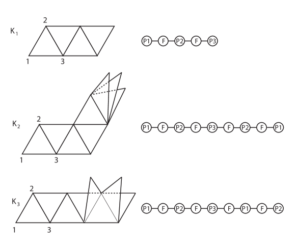
Figure 1. Three minimally branched complexes in $\mathcal{T}_{2}$ and their associated labelled graphs.

Example 2.7.

In Figure 2 we give two examples of maximally branched complexes $B_{1},B_{2}\in\mathcal{T}_{2}$ and their associated labelled graphs $\Gamma(B_{i})$. One can check by hand that $\Gamma(B_{2})$ weakly covers $\Gamma(B_{1})$. In fact $\Gamma(B_{1})$ is the minimal graph in this bisimilarity class. Corollary 1.2 generalizes this example.

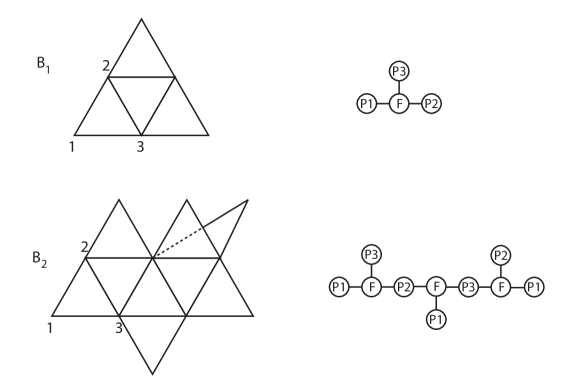
Figure 2. Two maximally branched complexes in $\mathcal{T}_{2}$ and their associated labelled graphs.

Proof of Corollary 1.2.

The minimal graph associated to an irreducible maximally branched right-angled $n$–tree group is a star consisting of a single central f–vertex connected to $n+1$ p–vertices, one of each color. ∎

Example 2.8.

For each $n\geq 2$, any pair of complexes $K,K^{\prime}\in\mathcal{T}_{n}$ which use only two ${\bf p}$–colors yield quasi-isometric groups and the minimal such graph, up to permutation of labels, corresponds to a graph of the form ${\bf p}1$—${\bf f}$—${\bf p}2$. Any such group is reducible; more generally, a group corresponding to a complex $K\in\mathcal{T}_{n}$ is reducible if and only if its graph uses less than $n+1$ ${\bf p}$–colors. See Figure 3 for an example of a group in the quasi-isometry class of such a $K\in\mathcal{T}_{2}$, but whose graph is not minimal.

The number of minimal graphs with $k$ ${\bf p}$–vertices chosen from a set of $3$ ${\bf p}$–colors grows with $k$. For $k=3$ there are two minimal graphs, for $k=4$ there are three, for $k=5$ there are twelve such graphs, and for $k=6$ there are forty-five.

Note there are two quasi-isometry types corresponding to graphs with one ${\bf p}$–vertex, one when the piece is just a simplex and the other when the piece is built from more than one simplex, and just one minimal graph with two ${\bf p}$–vertices, this is the example given in Figure 3 whose minimal graph is ${\bf p}1$—${\bf f}$—${\bf p}2$. Hence, there are exactly 65 quasi-isometry types of right-angled $2$–tree groups built from $6$ or less pieces.

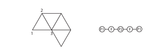
Figure 3. A complex in $\mathcal{T}_{2}$ built from three pieces and its associated labelled graph.

3. Bisimilar implies quasi-isometric

The following will prove the “if” direction of Theorem 1.1.

Theorem 3.1.

Fix $K,K^{\prime}\in\mathcal{T}_{n}$. If the graphs $\Gamma(K)$ and $\Gamma(K^{\prime})$ are bisimilar, then $A_{K}$ and $A_{K^{\prime}}$ are quasi-isometric.

Proof of Theorem 3.1.

Fix a pair of complexes $K,K^{\prime}\in\mathcal{T}_{n}$ for which $\Gamma(K)$ and $\Gamma(K^{\prime})$ are bisimilar and let $\Gamma$ denote the minimal graph in this bisimilarity class.

Each group $A_{K}$ and $A_{K^{\prime}}$ is represented as the fundamental group of the generalized “graph space” $X_{K}$ and $X_{K^{\prime}}$ (it need not be a manifold, since it has up to $(n+1)$ pieces glued together along each gluing torus), and is thus quasi-isometric to the universal cover of this space. Below we follow the same induction as in the proof of [BN, Theorem 3.2] to show that the universal covers of $X_{K}$ and $X_{K^{\prime}}$ are bilipschitz homeomorphic, implying the quasi-isometry of $A_{K}$ and $A_{K^{\prime}}$.

The universal cover of a piece of $X_{K}$ or $X_{K^{\prime}}$ is identified with $\tilde{S_{i}}\times{\mathbb{R}}^{n}$, where $S_{i}$ is one of a finite collection of compact riemannian surfaces with boundary (each of these is a sphere minus a finite number, at least three, of open disks). Note that these $S_{i}$ all have bilipschitz homeomorphic universal covers.

Let $X_{0}$ denote the universal cover of a fixed riemannian metric on a sphere minus three disks. Let $C$ be a finite set of “colors”. A bounded $C$-coloring on the boundary components of $X_{0}$ is an assignment of a color in $C$ to each boundary component of $X_{0}$ such that every point of $X_{0}$ is within a uniformly bounded distance of boundary components of every color. Choose a fixed boundary component of the universal cover, denoted $\partial_{0}X_{0}$. The following is Theorem 1.3 of [BN].

Theorem 3.2.

For any manifold $X$ bilipschitz homeomorphic to $X_{0}$ with a bounded $C$–coloring on the elements of $\partial X$, there exists $L$ and a function $\phi\colon{\mathbb{R}}\to{\mathbb{R}}$ such that for any $L^{\prime}$ and any color-preserving $L^{\prime}$–bilipschitz homeomorphism $\Phi_{0}$ from a boundary component $\partial_{0}X$ of $X$ to $\partial_{0}X_{0}$, then $\Phi_{0}$ extends to a $\phi(L^{\prime})$–bilipschitz homeomorphism $\Phi\colon X\to X_{0}$ which is $L$–bilipschitz on every other boundary component and which is a color-preserving map from $\partial X$ to $\partial X_{0}$.∎

Each piece of $K$ or $K^{\prime}$ is associated with some p–vertex $v$ of the minimal graph $\Gamma$; we then say the piece has type $v$, and similarly for the pieces of the geometric realizations $X_{K}$ and $X_{K^{\prime}}$ and their universal covers $\tilde{X}_{K}$ and $\tilde{X}_{K^{\prime}}$. We let $C_{v}$ denote the set of outgoing edges at the p–vertex $v$, so there is a natural $C_{v}$–labelling of the boundary components of any type $v$ geometric piece of $\tilde{X}_{K}$ or $\tilde{X}_{K^{\prime}}$.

Choose a number $L$ sufficiently large so that Theorem 3.2 applies for the universal cover of each of the $S_{i}$. Choose a bilipschitz homeomorphism from one type $v$ piece $\tilde{S}_{i}\times{\mathbb{R}}$ of $\tilde{X}_{K}$ to a type $v$ piece $X_{0}\times{\mathbb{R}}^{n}$ of $\tilde{X}_{K^{\prime}}$, preserving the (surface)$\times{\mathbb{R}}^{n}$ product structure and the $C_{v}$–colors of boundary components; this can be done since the graphs are bisimilar. We want to extend to a neighboring piece of $\tilde{X}_{K}$. On the common boundary ${\mathbb{R}}\times{\mathbb{R}}^{n}$ we have a map that is of the form $\phi_{1}\times\phi_{2}$ with $\phi_{1}$ and $\phi_{2}$ both bilipschitz. Since $\Gamma(K)$ and $\Gamma(K^{\prime})$ are bisimilar, each neighboring piece in $\tilde{X}_{K^{\prime}}$ has the same label as the corresponding piece in $\tilde{X}_{K}$ and thus we can extend over each neighboring piece by a product map. Further, by Theorem 3.2, we can assume this map preserves boundary colors and on the other boundaries of this piece is given by maps of the form $\phi^{\prime}_{1}\times\phi_{2}$ with $\phi^{\prime}_{1}$ $L$–bilipschitz. We do this for all neighboring pieces of our starting piece. Because of the flip, when we extend over the next layer we have maps on the outer boundaries that are $L$–bilipschitz in both base and fiber. We can thus continue extending outwards inductively to construct our desired bilipschitz map. ∎

4. Quasi-isometries preserve the decomposition into pieces

As described above, the group $A_{K}$ with $K\in\mathcal{T}_{n}$ is the fundamental group of a “graph space” $X_{K}$ whose universal cover $\tilde{X}_{K}$ is a quasi-isometric model for $A_{K}$. This $\tilde{X}_{K}$ has its geometric decomposition into pieces which overlap each other in separating flats. (Equivalently, the same decomposition is given directly on $A_{K}$ up to quasi-isometry by writing $A_{K}$ as the union of the cosets of the p–vertex groups of its geometric graph-of-groups decomposition.) The asymptotic cone $A_{\omega}$ of $A_{K}$ (which equals the asymptotic cone of $\tilde{X}_{K}$) admits a similar decomposition into subsets coming from asymptotic cones of the pieces of $A_{K}$, which we call pieces as well; note that the asymptotic cone of any piece is isometric to $T\times{\mathbb{R}}^{n}$ where $T$ is a metric tree (all the asymptotic cones we consider are taken with respect to an arbitrary, but fixed, choice of ultrafilter and scaling constants). Below, we apply Kapovich–Leeb’s argument that quasi-isometries preserve the geometric decomposition of $3$-manifolds [KL2], to the present situation.

The following lemma in the case $n=1$ was proven in [KL1, Lemma 2.14]; the same argument holds to prove:

Lemma 4.1.

Fix a metric tree $T$. If $f\colon{\mathbb{R}}^{n+1}\to T\times{\mathbb{R}}^{n}$ is a bilipschitz embedding, then the image, $f({\mathbb{R}}^{n+1})$, is a subset which is isometric to ${\mathbb{R}}^{n+1}$.∎

An immediate corollary of this lemma is that any subset of $A_{\omega}$ which is contained in the asymptotic cone of one of the pieces and which is bilipschitz to ${\mathbb{R}}^{n+1}$ must actually be an isometrically embedded flat.

In a similar direction, the following also holds as in [KL2, Lemma 3.3]:

Lemma 4.2.

Let $T$ be a geodesically complete tree and $C\subseteq{\mathbb{R}}^{n}$ a closed subset. If $f\colon C\to T\times{\mathbb{R}}^{n}$ is a bilipschitz embedding whose image separates, then $C={\mathbb{R}}^{n}$ and the projection of the image to $T$ is contained in a segment with no branch point in its interior. In particular, if $T$ branches everywhere, then the image is a fiber $\{t\}\times{\mathbb{R}}^{n}$.∎

The arguments of [KL2] then apply to show that any bilipschitz embedding of a tree cross ${\mathbb{R}}^{n}$ into $A_{\omega}$ must lie inside a piece, which then implies:

Proposition 4.3.

Let $K,K^{\prime}\in\mathcal{T}_{n}$ and let $A_{\omega},A_{\omega}^{\prime}$ denote asymptotic cones of $A_{K},A_{K^{\prime}}$. Let $\phi\colon A_{\omega}\to A_{\omega}^{\prime}$ be a bilipschitz homeomorphism. Then $\phi$ sends pieces to pieces and separating flats to separating flats.∎

Using the $\operatorname{CAT}(0)$ structure on $A_{\omega}$ and identical arguments as for [KL2, Theorem 4.6], one shows that any quasiflat which is not sublinearly close to a separating flat must diverge from it linearly and in particular that any quasi-isometry from $A_{K}$ to $A_{K^{\prime}}$ sends flats to flats. As in [KL2, Theorem 1.1], this result applied in the present context implies the following theorem:

Theorem 4.4.

Let $\phi\colon A_{K}\to A_{K^{\prime}}$ be a quasi-isometry. Then $\phi$ preserves the geometric decompositions of $\tilde{X}_{K}$ and $\tilde{X}_{K^{\prime}}$ in the following sense: for any geometric piece $X$ of $\tilde{X}_{K}$ there exists a geometric piece $X^{\prime}$ of $\tilde{X}_{K^{\prime}}$ within a uniformly bounded Hausdorff distance from $\phi(X)$. Moreover, $\phi$ induces an isomorphism of trees dual to the geometric decomposition of $\tilde{X}_{K}$ and $\tilde{X}_{K^{\prime}}$.∎

To complete the “only if” direction of Theorem 1.1, we must show the induced map of trees also preserves the p–vertex labelling up to a permutation of labels, since this dual tree is then the unique labelled tree in the bisimilarity class corresponding to the associated Artin group. To do this, it suffices to show that if we know the geometric decomposition of $\tilde{X}_{K}$ up to quasi-isometry then we can tell when two p–vertices $v$ and $v^{\prime}$ of the decomposition tree have the same color.

The path from $v$ to $v^{\prime}$ consists of alternating p– and f–vertices,

$$v=v_{0},w_{1},v_{1},\dots,w_{r},v_{r}=v^{\prime}\,,$$

say. The $T^{n}$ in the geometric piece for vertex $v_{0}$ defines an $n$–dimensional sub-flat ${\mathbb{R}}^{n}$ of the flat ${\mathbb{R}}^{n+1}$ in $A_{\omega}$ corresponding to $w_{1}$. As we move along the path we intersect this subflat repeatedly with the projection to this flat of the codimension–$1$ subflats for the vertices $v_{1},v_{2},\dots$ (alternatively, this can be interpreted as the coarse intersection of the subflats associated to the centers of the respective pieces; hence this is quasi-isometrically invariant since the center in a piece corresponds to the coarse intersection of all the maximal flats). Whenever we pass a $v_{i}$ of a color we have not yet seen, the dimension of the intersection drops by $1$. Otherwise, we know we have already seen the color along the path, and by using the same procedure to check backwards along the path from $v_{i}$, we can find which vertex had the same color. If it was not $v_{0}$ we then continue the same way along the path. In this way we either show that $v_{r}$ has the same color as $v_{0}$, or the dimension of our subspace has reached $0$ by the time we get to $v_{r}$, in which case we have seen every color along the path. By induction we can assume that we have already determined which $v_{i}$’s that are closer together along the path have the same color. But then, by checking forwards along the path from $v_{0}$ and backwards from $v_{r}$ we can tell that they both have different colors from every other $v_{i}$ along the path, so must have the same color.

This completes the proof of the “only if” direction of Theorem 1.1, and since the “if” direction is Theorem 3.1, Theorem 1.1 is proved.∎

Remark 4.5.

The above argument shows that the construction of labels in Section 2.2 could be done purely geometrically. As an example to see this, compare the example in Figure 4 to example B1 in Figure 2. To see how to label the shaded piece, $N$, consider the associated space $\tilde{X}_{B_{1}^{\prime}}$, and note that in this space $N$ has three-dimensional intersection with the $P3$ piece and two-dimensional intersection with both the pieces labelled $P1$ and $P2$. The intersection of the torus associated to the center of $N$ with the center of $P1$ is one dimensional, while its intersection with the center of $P2$ is trivial. Since a path starting from the $P1$ or $P3$ piece would not need to traverse all the labels, whereas a path starting at the $P2$ piece would have traversed the $P2$ and $P3$ labels, we thus see that the $N$ must be labelled by a 1, as given by the labelling in Section 2.2.

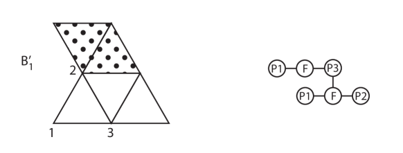
Figure 4. Compare with example B1 in Figure 2.

References

- [BDM] J. Behrstock, C. Druţu, and L. Mosher. Thick metric spaces, relative hyperbolicity, and quasi-isometric rigidity. Math. Ann. 344(2009), 543–595.
- [BN] J. Behrstock and W. Neumann. Quasi-isometric classification of graph manifold groups. Duke Math. J. 141(2008), 217–240.
- [BJN] Jason A. Behrstock, Tadeusz Januszkiewicz, and Walter D. Neumann. Commensurability and QI classification of free products of finitely generated abelian groups. Proc. Amer. Math. Soc. 137(2009), 811–813.
- [BKS] M. Bestvina, B. Kleiner, and M. Sageev. The asymptotic geometry of right-angled Artin groups. I. Geometry & Topology 12(2008), 1653–1699.
- [Cha] Ruth Charney. An introduction to right-angled Artin groups. Geom. Dedicata 125(2007), 141–158.
- [CD] Ruth Charney and Michael W. Davis. Finite s for Artin groups. In Prospects in topology (Princeton, NJ, 1994), volume 138 of Ann. of Math. Stud., pages 110–124. Princeton Univ. Press, Princeton, NJ, 1995.
- [Gro] M. Gromov. Groups of polynomial growth and expanding maps. IHES Sci. Publ. Math. 53(1981), 53–73.
- [HM] Susan Hermiller and John Meier. Artin groups, rewriting systems and three-manifolds. J. Pure Appl. Algebra. 136 (1999), 141–156.
- [KL1] M. Kapovich and B. Leeb. On asymptotic cones and quasi-isometry classes of fundamental groups of nonpositively curved manifolds. Geom. Funct. Anal. 5(1995), 582–603.
- [KL2] M. Kapovich and B. Leeb. Quasi-isometries preserve the geometric decomposition of Haken manifolds. Invent. Math. 128(1997), 393–416.
- [PW] P. Papasoglu and K. Whyte. Quasi-isometries between groups with infinitely many ends. Comment. Math. Helv. 77(2002), 133–144.