Exact solution for a quantum compass ladder

Abstract

We introduce a spin ladder with antiferromagnetic Ising ZZ interactions along the legs, and interactions on the rungs which interpolate between the Ising ladder and the quantum compass ladder. We show that the entire energy spectrum of the ladder may be determined exactly for finite number of spins $2N$ by mapping to the quantum Ising chain and using Jordan-Wigner transformation in invariant subspaces. We also demonstrate that subspaces with spin defects lead to excited states using finite size scaling, and the ground state corresponds to the quantum Ising model without defects. At the quantum phase transition to maximally frustrated interactions of the compass ladder, the ZZ spin correlation function on the rungs collapses to zero and the ground state degeneracy increases by 2. We formulate a systematic method to calculate the partition function for a mesoscopic system, and employ it to demonstrate that fragmentation of the compass ladder by kink defects increases with increasing temperature. The obtained heat capacity of a large compass ladder consisting of $2N=104$ spins reveals two relevant energy scales and has a broad maximum due to dense energy spectrum. The present exact results elucidate the nature of the quantum phase transition from ordered to disordered ground state found in the compass model in two dimensions.

Published in: Phys. Rev. B 80, 014405 (2009).

I Introduction

Spin ladders play an important role in quantum magnetism. Interest in them is motivated by their numerous experimental realizations in transition metal oxides Dag99 and has increased over the last two decades. One of recently investigated realizations of spin ladders are Sr_n-1Cu_n+1O_2n cuprates (with $n=3,5,7,\cdots$),Gop94 and the simplest of them, a spin ladder with two legs connected by rungs, is realized in Sr₂Cu₄O₆. Excitation spectra of such antiferromagnetic (AF) spin ladders are rich and were understood only in the last decade. They consist of triplet excitations, bound states and two-particle continuum,Tre00 and were calculated in unprecedented detail for quantum AF spin $S=1/2$ two-leg ladder employing optimally chosen unitary transformation.Kne01 In some of spin ladder systems charge degrees of freedom also play a role, as for instance in $\alpha^{\prime}$-NaV₂O₅, where AF order and charge order coexist in spin ladders with two legs,Hor98 or in the Cu–O planes of La_xSr_14-xCu₂₄O₄₁, where spin and charge order coexist for some values of $x$.Woh07 This advance in the theoretical understanding of the ground states and excitation spectra of spin ladders is accompanied by recent experimental investigations of triplon spectra by inelastic neutron scattering Not07 of almost perfect spin ladders in La₄Sr₁₀Cu₂₄O₄₁. Finally, in the theory spin ladders could serve as a testing ground for new (ordered or disordered) phases which might arise for various frustrated exchange interactions.Pen07

A particularly interesting situation arises when frustration of spin interactions may be tuned by varying strength of certain coupling constants, and could thus exhibit transitions between ordered and disordered phases. On the one hand, periodically distributed frustrated Ising interactions do not suffice to destroy magnetic long-range order in a two-dimensional (2D) system, but only reduce the temperature of the magnetic phase transition.Lon80 On the other hand, when the model is quantum, increasing frustration of exchange interactions may trigger a quantum phase transition (QPT), as for instance in the one-dimensional (1D) compass model.Brz07 Physical realizations of frustrated interactions occur in 2D and three-dimensional spin-orbital models derived for Mott insulators in transition metal oxides in the orbital part of the superexchange. In such models frustration is intrinsic and follows from the directional nature of orbital interactions.Fei97 Usually such frustration is removed either by Hund’s exchange $J_{H}$ or by Jahn-Teller orbital interactions, but when these terms are absent it leads to a disordered orbital liquid ground state. Perhaps the simplest realistic example of this behavior is the (Kugel-Khomskii) model for Cu²⁺ ions in $d^{9}$ electronic configuration at $J_{H}=0$, where a disordered ground state was found.Fei98 Examples of such disordered states are either various valence-bond phases with singlet spin configurations on selected bonds,Mat04 or orbital liquids established both in $t_{2g}$ systemsKha00 and in $e_{g}$ systems.Fei05 Characteristic features of spin-orbital models are enhanced quantum effects and entanglement, Ole06 so their ground states cannot be predicted using mean-field decoupling schemes. Also in doped systems some unexpected features emerge for frustrated orbital superexchange interactions, and the quasiparticle states are qualitatively different from those arising in the spin $t$–$J$ model. vdB00 Therefore, it is of great interest to investigate spin models with frustrated interactions which stand for the orbital part of the superexchange, particularly when such models could be solved exactly.

Although the orbital superexchange interactions are frequently Ising-like, they lead to quantum models with intrinsically frustrated exchange models as different orbital components interact depending on the bond orientation in real space.vdB04 A generic case of such frustrated interactions is the so-called 2D quantum compass model, Kho03 which was recently investigated numerically. Mil05 ; Wen08 Although orbital superexchange interactions in Mott insulators are typically AF,Fei97 ; Fei98 ; Mat04 ; Kha00 a similar frustration concerns also ferromagnetic (FM) interactions, and a QPT was also found in the compass model with FM interactions.Che07

The 1D variant of the compass model with alternating interactions of $z$-th and $x$-th spin components on even and odd bonds was solved exactly by an analytical method,Brz07 and entanglement in the ground state was analyzed recently.You08 We note that the 1D compass model (the model of Ref. Brz07, in the limit of equal and alternating interactions on the bonds) is equivalent to the 1D anisotropic XY model, solved in the seventies.Per75 An exact solution of the 1D compass model demonstrates that certain nearest-neighbor spin correlation functions change discontinuously at the point of a QPT when both types of interactions have the same strength. This somewhat exotic behavior follows because the QPT occurs at the multicritical point in the parameter space.Eri09 A similar discontinuous behavior of nearest-neighbor spin correlations was also found numerically for the 2D compass model.Kho03 While small anisotropy of interactions leads to particular short-range correlations dictated by the stronger interaction, in both 1D and 2D compass model one finds a QPT to a highly degenerate disordered ground state when the interactions are balanced.

The purpose of this paper is to present an exact solution of the compass model on a spin ladder, with ZZ Ising interactions between $z$-th spin components along the ladder legs, and interactions on the rungs which gradually evolve from ZZ Ising interactions to XX Ising ones. In this way the interactions interpolate between the classical Ising spin ladder and the quantum compass ladder with frustrated interactions. The latter case will be called compass ladder below — it stands for a generic competition between orbital interactions on different bonds and can serve to understand better the physical consequences of the frustrated orbital superexchange.

The paper is organized as follows. The model and its invariant dimer subspaces are introduced in Sec. II. Next the ground state and the lowest excited states of the model are found in Sec. III by solving the model in all nonequivalent subspaces. Thereby we discuss the role played by defects in spin configuration and show that the ground state is obtained by solving the 1D quantum Ising (pseudospin) model (QIM). Using an example of a finite system, we provide an example of the energy spectrum, and next extrapolate the ground state energy obtained for finite systems to the thermodynamic limit. We also present the changes of spin correlations at the QPT, and derive the long-range spin correlations. Next we construct canonical ensemble for the spin ladder in Sec. IV and present the details concerning the calculation of energies in the appendix. The constructed partition function is used to derive such thermodynamic properties of the compass ladder as the temperature variation of spin correlations, and the average length of fragmented chains separated by kinked areas in Sec. V. In Sec. VI we present the evolution of heat capacity $C_{V}$ when interactions change from the Ising to compass ladder for a small ladder of $N=8$ spins, and next analyze $C_{V}$ for a large (mesoscopic) compass ladder of $2N=104$ spins. While the characteristic excitation energies responsible for the maxima in heat capacities can be deduced from the energy spectrum for $N=8$ spins, generic features of excitations follow from the form of $C_{V}$ in case of the mesoscopic compass ladder. Final discussion and summary of the results are given in Sec. VII.

II Compass model on a ladder

We consider a spin ladder with $N$ rungs $\langle 2i-1,2i\rangle$ labelled by $i=1,2,\cdots,N$. The interactions along ladder legs are Ising-like with AF coupling $J$ between $z$-th spin components ($\sigma_{i}^{z}\sigma_{i+1}^{z}$), while AF interactions on the rungs interpolate between the Ising coupling of $z$-th ($2\sigma_{n-1}^{z}\sigma_{n+1}^{z}$) and $x$-th ($2\sigma_{n-1}^{x}\sigma_{n+1}^{x}$) spin components,

$${\cal H}(\alpha) = 2J\sum_{i=1}^{N}\left\{\alpha\sigma^{x}_{2i-1}\sigma^{x}_{2i}+(1-\alpha)\sigma^{z}_{2i-1}\sigma^{z}_{2i}\right\}$$ (1)

$$+ J\sum_{i=1}^{N}\left(\sigma^{z}_{2i-1}\sigma^{z}_{2i+1}+\sigma^{z}_{2i}\sigma^{z}_{2i+2}\right)\,,$$

by varying parameter $0\leq\alpha\leq 1$. We assume periodic boundary conditions along the ladder legs, i.e., $\sigma^{z}_{2N+1}\equiv\sigma^{z}_{1}$ and $\sigma^{z}_{2N+1}\equiv\sigma^{z}_{2}$. The factor of two for the interactions on the rungs $\propto 2J$ was chosen to guarantee the same strength of interactions on the rungs (with only one rung neighbor of each spin) as along the ladder legs (with two leg neighbors). Increasing $\alpha$ gradually modifies the interactions on the rungs and increases frustration. For $\alpha=0$ one finds the reference Ising ladder, while at $\alpha=1$ the interactions describe a competition between frustrated ZZ interactions along the ladder legs and 2XX interactions on the rungs, characteristic of the compass ladder. A representative compass ladder with $N=4$ rungs (i.e., $2N=8$ spins) is shown in Fig. 1.

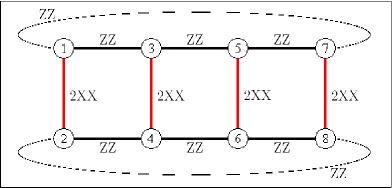
Figure 1: (Color online) Schematic view of the quantum compass ladder with $N=4$ rungs, described by Hamiltonian (1) with $\alpha=1$. Interactions along the ladder legs labeled as $ZZ$ (horizontal lines) are $\sigma^{z}_{2i-1}\sigma^{z}_{2i+1}$ (upper leg) and $\sigma^{z}_{2i}\sigma^{z}_{2i+2}$ (lower leg). The interactions along the rungs labeled as $2XX$ (vertical lines) are $2\sigma^{x}_{2i-1}\sigma^{x}_{2i}$ (the factor of 2 simulates the periodic boundary condition along the rungs). Dashed lines indicate periodic boundary conditions along the ladder legs.

To solve the spin ladder given by Eq. (1) in the range of $0\leq\alpha\leq 1$ we notice that $[{\cal H}(\alpha),\sigma_{2i-1}^{z}\sigma_{2i}^{z}]\equiv 0$. Therefore we have a set of $N$ symmetry operators,

$$R_{i}\equiv\sigma_{2i-1}^{z}\sigma_{2i}^{z}\,,$$ (2)

with respective eigenvalues $r_{i}=\pm 1$. Each state of the system can be thus written in a basis of $\sigma^{z}_{i}$ eigenvectors $\left|s_{1},s_{2},s_{3},\ldots,s_{2N}\right\rangle$ fixed by strings of quantum numbers $s_{i}=\pm 1$. These vectors can be parametrized differently by a new set of quantum numbers $\{t_{i}\}$ and $\{r_{i}\}$, with $i=1,2,\cdots,N$; they are related to the old ones by the formulae: $t_{i}\equiv s_{2i-1}$ and $r_{i}\equiv s_{2i-1}s_{2i}$. Now we introduce new notation for the basis states

$$\left|t_{1},t_{2},\ldots,t_{N}\right\rangle_{r_{1}r_{2}\cdots r_{N}}\equiv\left|t_{1},t_{1}r_{1},t_{2},t_{2}r_{2},\ldots,t_{N},t_{N}r_{N}\right\rangle\ ,$$ (3)

where the right-hand side of Eq. (3) is the state $\left|s_{1},s_{2},s_{3},\ldots,s_{2N}\right\rangle$ written in terms of variables $\{t_{i}\}$ and $\{r_{i}\}$, and the left-hand side defines new notation. This notation highlights the different role played by $r_{i}$’s, which are conserved quantities, and by $t_{i}$’s, being new pseudospin variables. For states like in Eq. (3), we define new pseudospin operators $\tau_{i}^{z}$ and $\tau_{i}^{x}$ acting on $\{t_{i}\}$ quantum numbers as Pauli matrices, e.g. for $i=1$:

$$\tau_{1}^{x}|t_{1},t_{2},\ldots,t_{N}\rangle_{r_{1}r_{2}\cdots r_{N}} = |-t_{1},t_{2},\ldots,t_{N}\rangle_{r_{1}r_{2}\cdots r_{N}}\ ,$$

$$\tau_{1}^{z}|t_{1},t_{2},\ldots,t_{N}\rangle_{r_{1}r_{2}\cdots r_{N}} = t_{1}|t_{1},t_{2},\ldots,t_{N}\rangle_{r_{1}r_{2}\cdots r_{N}}\ .$$

A similar transformation was introduced for a frustrated spin-$1/2$ chain by Emery and Noguera,Eme88 who showed that it can by mapped onto an Ising model in a transverse field. Recently this procedure was used to investigate quantum criticality in a two-leg strongly correlated ladder model at quarter filling.Laa08

The Hamiltonian can be now written in a common eigenbasis of $R_{i}$ (2) operators by means of $\{\tau_{i}^{x},\tau_{i}^{z}\}$ operators. In a subspace labelled by a string $r_{1},r_{2},\cdots,r_{N}$, the reduced form of the Hamiltonian is

$${\cal H}_{r_{1}r_{2}\cdots r_{N}}(\alpha) \equiv J\sum_{i=1}^{N}\left\{(1+r_{i}r_{i+1})\tau_{i}^{z}\tau_{i+1}^{z}+2\alpha\tau_{i}^{x}\right\}$$ (5)

$$+ 2JC_{\vec{r}}(\alpha)\ ,$$

with a constant

$$C_{\vec{r}}(\alpha)=(1-\alpha)\sum_{i=1}^{N}r_{i}\,,$$ (6)

and periodic boundary condition $\tau_{N+1}^{z}\equiv\tau_{1}^{z}$. This leads to the exactly solvable QIM with transverse field,Lie61 ; Dzi05 ; Mat06 if only $r_{i}\equiv 1$ or $r_{i}\equiv-1$. Otherwise there are always some $\tau^{z}_{i}\tau^{z}_{i+1}$ interactions missing (defects created in the chain) and we obtain a set of disconnected quantum Ising chains with loose ends and different lengths. The bonds with no pseudospin interactions may stand next to each other, so in an extreme case when $r_{i+1}=-r_{i}$ for all $i$, one finds no Ising bonds and no chains appear.

One may easily recognize that the ground state of the spin ladder described by Hamiltonian (1) lies in a subspace with $r_{i}\equiv-1$ for $\alpha<1$. First of all, $r_{i}\equiv-1$ minimizes $C_{\vec{r}}(\alpha)$, see Eq. (6). To understand a second reason which justifies the above statement let us examine a partial Hamiltonian (open chain) of the form

$${\cal H}(\alpha,L)=2J\sum_{i=1}^{L-1}\tau_{i}^{z}\tau_{i+1}^{z}+2J\alpha\sum_{i=1}^{L}\tau_{i}^{x}\ ,$$ (7)

with $2\leq L\leq N-1$. Note that it appears generically in Eq. (5) and consists of two terms containing pseudospin operators $\{\tau^{x}_{i}\}$ and $\{\tau^{z}_{i}\}$. Let us call them ${\cal H}^{x}$ and ${\cal H}^{z}$ and denote the ground state of ${\cal H}^{x}$ as $|x\rangle$ with energy $E_{x}$. The mean value of ${\cal H}(\alpha,L)$ in state $|x\rangle$ is also $E_{x}$ because every $\tau_{i}^{z}$ operator has zero expectation value in state $|x\rangle$, i.e., $\langle x|\tau_{i}^{z}|x\rangle=0$. However, we know that $|x\rangle$ is not an eigenvector of ${\cal H}(\alpha,L)$ which implies that ${\cal H}(\alpha,L)$ must have a lower energy than $E_{x}$ in the ground state. This shows that the presence of $\tau_{i}^{z}\tau_{i+1}^{z}$ bonds in the Hamiltonian ${\cal H}(\alpha,L)$ lowers the energy of bare ${\cal H}^{x}$. One may also expect that this energy decreases with increasing length $L$ of the chain, and is proportional to $L$ in the thermodynamic limit. The numerical evidence for this are plots of the ground state energy versus $L$ presented in section 3. Looking at Hamiltonian (5) we see that the longest chains of the type (7) appear in subspaces with $r_{i}\equiv-1$ and $r_{i}\equiv 1$, but the constant term $C_{\vec{r}}(\alpha)$ favors $r_{i}\equiv-1$ if only $\alpha<1$. For $\alpha=1$ the ground state can be in both subspaces, and its degeneracy follows, see below.

III Energy spectra in invariant subspaces

III.1 Quantum Ising model

To find the ground state of spin ladder (1) we need to solve the QIM that arises from Eq. (5) when $r_{i}\equiv-1$. Thus we need to diagonalize the Hamiltonian of the form

$${\cal H}_{\rm QIM}(\beta,\alpha)=2J\sum_{i=1}^{N}(\beta\tau_{i}^{z}\tau_{i+1}^{z}+\alpha\tau_{i}^{x})\ ,$$ (8)

which is related to our original problem by the formula

$${\cal H}_{-1-1\cdots-1}={\cal H}_{\rm QIM}(1,\alpha)-2NJ(1-\alpha)\ .$$ (9)

The formal parameter $\beta$ is introduced for convenience and will be used to determine the correlation functions along the ladder legs by differentiation, see below. The standard way of solving ${\cal H}_{\rm QIM}$ starts with Jordan–Wigner (JW) transformation. This non–linear mapping replacing spin operators by spinless fermions is of the form

$$\tau_{j}^{z} = (c_{j}+c_{j}^{\dagger}){\prod_{i<j}}(1-2c_{i}^{\dagger}c_{i})\ ,$$

$$\tau_{j}^{x} = (1-2c_{j}^{\dagger}c_{j})\ .$$ (10)

The boundary condition for fermion operators $\{c_{i}\}$ after inserting them into ${\cal H}_{\rm QIM}$ (8) is antiperiodic for even and periodic for odd number of JW quasiparticles in the chain. The operator ${\cal P}$ of the parity of fermions,

$${\cal P}=\prod_{i=1}^{N}\,(1-2c_{i}^{\dagger}c_{i})\ ,$$ (11)

corresponds to the operation of flipping all spins along the $z$-th axis and commutes with ${\cal H}_{\rm QIM}$. Therefore, the Hamiltonian can be split into two diagonal blocks, for even $(+)$ and odd $(-)$ number of JW fermions by means of projection operators $\frac{1}{2}(1\pm{\cal P})$. Therefore we write

$${\cal H}_{\rm QIM}=\frac{1}{2}(1+{\cal P}){\cal H}^{+}+\frac{1}{2}(1-{\cal P}){\cal H}^{-}\ ,$$ (12)

where

$${\cal H}^{\pm} = 2J\sum_{i=1}^{N}\left\{\beta(c_{i}^{\dagger}-c_{i})(c_{i+1}^{\dagger}+c_{i+1})-2\alpha c_{i}^{\dagger}c_{i}\right\}$$ (13)

$$+ 2JN\alpha\ ,$$

with two different boundary conditions: $c_{N+1}=\mp c_{1}$ for ($\pm$) subspaces. Let us point out that the only consequence of the nonlinearity of the JW transformation is the minus sign which appears in the first bracket multiplying $\beta$. This is thanks to one–dimensionality and only nearest-neighbor interactions in the reduced Hamiltonian (5), but is not the case for the original Hamiltonian (1).

Next step is the Fourier transformation,

$$c_{j}=\frac{1}{\sqrt{N}}\sum_{k}e^{ijk}c_{k}\,,$$ (14)

with quasimomenta $k=\pm(2l-1)\pi/N$ $[l=1,2,\cdots,N/2]$ in an even subspace $(+)$, and $k=0,\pi,\pm 2l\pi/N$ $[l=1,2,\cdots,(N/2-1)]$ in an odd one $(-)$. After transforming the operators in Eq. (13) we obtain ${\cal H}^{\pm}$ in a block diagonal form,

$${\cal H}^{\pm} = 4J{\sum_{k}}^{\pm}(\beta\cos k-\alpha)c^{\dagger}_{k}c_{k}$$ (15)

$$+ 2J{\sum_{k}}^{\pm}\beta(c^{\dagger}_{k}c^{\dagger}_{-k}e^{ik}+h.c.)+2JN\alpha\,.$$

Diagonalization is completed by a Bogoliubov transformation, defining new fermion operators ${\gamma}^{\dagger}_{k}\equiv\alpha_{k}c^{\dagger}_{k}+\beta_{k}c_{-k}$ (for $k\neq 0,\pi$, while the operators $c_{0}$ and $c_{\pi}$ have no partner and are left untransformed). Transformation coefficients $\alpha_{k}$ and $\beta_{k}$ are obtained from the condition

$$\left[{\cal H}_{\rm QIM},\gamma^{\dagger}_{k}\right]=\omega_{k}\gamma^{\dagger}_{k}\,,$$ (16)

which is an eigenproblem in linear space spanned by operators $c_{k}^{\dagger}$ and $c_{-k}$. We get two eigenvectors $(\alpha_{k},\beta_{k})$, corresponding to the quasiparticle operators ${\gamma}^{\dagger}_{k}$ and ${\gamma}_{-k}$, and two corresponding eigenvalues $\omega_{k}=\pm E_{k}$, with

$$E_{k}(\beta,\alpha)=4J\left\{\alpha^{2}+\beta^{2}-2\alpha\beta\cos k\right\}^{1/2}\,.$$ (17)

Therefore, the Hamiltonian is brought to the diagonal form in both subspaces

$${\cal H}^{+} = {\sum_{k}}^{+}E_{k}\left(\gamma^{\dagger}_{k}\gamma_{k}-\frac{1}{2}\right)\ ,$$ (18)

$${\cal H}^{-} = {\sum_{k}}^{-}E_{k}\left(\gamma^{\dagger}_{k}\gamma_{k}-\frac{1}{2}\right)+4J(\beta-\alpha)c^{\dagger}_{0}c_{0}$$ (19)

$$- 4J(\beta+\alpha)c^{\dagger}_{\pi}c_{\pi}+4J\alpha\ .$$

We still need to transform the parity operator ${\cal P}$. Luckily, the Fourier transformation does not change its form and to see that so does the Bogoliubov transformation, one can look at the vacuum state $|0\rangle$ for quasiparticle operators $\gamma_{k}$. From the condition $\gamma_{k}|0\rangle=0$ for all $k$ we get

$$|0\rangle=\prod_{k}\,\left(\bar{\alpha}_{k}+\bar{\beta}_{k}c_{-k}^{\dagger}c_{k}^{\dagger}\right)|vac\rangle\ ,$$ (20)

where $|vac\rangle$ is a true vacuum state for JW fermions or a state with all spins up. From the form of $|0\rangle$ we see that it contains a superposition of all even numbers of quasiparticles $c_{k}^{\dagger}$, and the total quasiparticle number is not fixed. Acting on the vacuum with a single creation operator $\gamma_{k}^{\dagger}$ we obtain a state with odd number of JW fermions, because $\gamma_{k}^{\dagger}$ is a linear combination of a creation $c_{k}^{\dagger}$ and annihilation $c_{-k}$ operator of a single fermion. In this way one may get convinced that the parity of quasiparticles $\gamma_{k}^{\dagger}$ and $c_{k}^{\dagger}$ is the same.

III.2 Ground state and the energy spectrum

Figure 2: Eigenenergies $E_{n}$ of the spin ladder (1) of Fig. 1 with $N=4$ rungs for increasing $\alpha$, obtained by exact diagonalization. Different panels show energies in invariant subspaces of the effective Hamiltonian (5), with $1$ and $\bar{1}$ standing for positive or negative values of $r_{i}$: (a) $\bar{1}\bar{1}\bar{1}\bar{1}$, (b) $1\bar{1}\bar{1}\bar{1}$, (c) $11\bar{1}\bar{1}$, (d) $1\bar{1}1\bar{1}$, (e) $111\bar{1}$ and (f) $1111$. While the subspaces (a) and (f) are unique, other subspaces are equivalent by symmetry to those shown in panels (b)–(e), resulting in total spectrum of 256 eigenstates. Quantum phase transition occurs at $\alpha=1$, where the lowest eigenenergies in the subspaces (a) and (f) become degenerate. In the thermodynamic limit $N\to\infty$ the spectrum changes qualitatively — the two lowest energies in the subspaces $\bar{1}\bar{1}\bar{1}\bar{1}$ and $1111$ are degenerate and the ground state from the subspace (b) ($1\bar{1}\bar{1}\bar{1}$) becomes the first excited state of the spin ladder.

From the diagonal form of the QIM Hamiltonian given by Eq. (18) we see that the ground state of spin ladder (1) is simply $|0\rangle$ in subspace $r_{i}\equiv-1$ (or $r_{i}\equiv 1$ when $\alpha=0$). For the ground state energy, one uses Eq. (9) to get

$$E_{-1-1\cdots-1}=E_{\rm QIM}(1,\alpha)-2NJ(1-\alpha)\ ,$$ (21)

with $E_{\rm QIM}(1,\alpha)$ given in the thermodynamic limit by an integral

$$E_{\rm QIM}(\beta,\alpha)=-\frac{N}{2\pi}\int_{0}^{\pi}dk\;E_{k}(\beta,\alpha)\,.$$ (22)

The ground state in the absence of transverse field (at $\alpha=0$) is doubly degenerate — it is given by two possible Néel states. At finite $\alpha>0$, this degeneracy is removed, and the sum of the two Néel states (symmetric state), $|0_{+}\rangle$, is the ground state, while their difference (antisymmetric state) becomes the first excited state. This first excited state, $|0_{-}\rangle=\gamma_{\pi}^{\dagger}|0_{+}\rangle$, stems from the same subspace and belongs to the spectrum of ${\cal H}^{-}$. The splitting of the states $|0_{+}\rangle$ and $|0_{-}\rangle$ increases with $\alpha$, see Fig. 2(a). For finite $N$ and $\alpha>0$ there is always finite energy difference between the energies of $|0_{+}\rangle$ and $|0_{-}\rangle=\gamma_{\pi}^{\dagger}|0_{+}\rangle$ states. However, in the thermodynamic limit $N\to\infty$, this energy gap vanishes for $\alpha\leq 1$ and starts to grow as $4J\alpha$ at $\alpha=1$.

The full spectrum for the ladder with $N=4$ rungs belongs to six classes of subspaces equivalent by symmetry — it is depicted in Fig. 2. With increasing $\alpha$ the spectrum changes qualitatively from discrete energy levels of the classical Ising ladder at $\alpha=0$, with the ground state energy per spin equal $-2J$, to a narrower and quasi–continuous spectrum when the quantum compass ladder at $\alpha=1$ is approached, with the ground state energy $-4J/\pi$ per spin. At the $\alpha=1$ point one finds an additional symmetry; subspaces indexed by $\vec{r}$ and $-\vec{r}$ are then equivalent which makes each energy level at least doubly degenerate.

III.3 Correlation functions

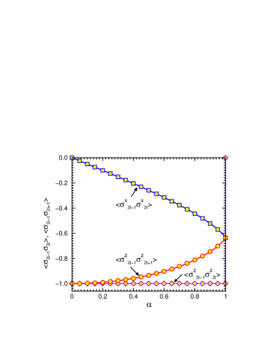
Figure 3: (Color online) Nearest neighbor correlation functions in the ground state for spin ladder (1) in the thermodynamic limit $N\to\infty$. For increasing $\alpha$ spin correlations $\langle\sigma_{2i-1}^{x}\sigma_{2i}^{x}\rangle$ on the rungs decrease from zero to $-2/\pi$. At the same time, AF correlations $\langle\sigma_{2i-1}^{z}\sigma_{2i+1}^{z}\rangle$ along the ladder legs gradually weaken (increase from the classical value $-1$ at $\alpha=0$ to $-2/\pi$ at $\alpha=1$), and become degenerate with the rung $\langle\sigma_{2i-1}^{x}\sigma_{2i}^{x}\rangle$ correlations at the quantum critical point $\alpha=1$. Correlation function $\langle\sigma_{2i-1}^{z}\sigma_{2i}^{z}\rangle$ on the rungs, directly related to the subspace indices $r_{i}$, remains constant $(\langle\sigma_{2i-1}^{z}\sigma_{2i}^{z}\rangle=-1)$ in the entire range of $\alpha<1$, and jumps to $0$ at $\alpha=1$.

All the nontrivial nearest neighbor spin correlation functions in the ground state can be determined by taking derivatives of the ground state energy $E_{\rm QIM}(\beta,\alpha)$ (22) with respect to $\alpha$ or $\beta$, while the others are evident from the construction of the subspaces. In this way one finds $\langle\sigma^{z}_{2i-1}\sigma^{z}_{2i+1}\rangle$ correlation along the legs and $\langle\sigma^{x}_{2i-1}\sigma^{x}_{2i}\rangle$ along the rungs, shown in Fig. 3. Spin correlations $\langle\sigma^{z}_{2i-1}\sigma^{z}_{2i+1}\rangle$ along the legs increase from the classical value $-1$ up to $-2/{\pi}$ for $\alpha=1$. By symmetry, both ladder legs are equivalent and $\langle\sigma^{\alpha}_{2i-1}\sigma^{\alpha}_{2i+1}\rangle=\langle\sigma^{\alpha}_{2i}\sigma^{\alpha}_{2i+2}\rangle$ for $\alpha=x,z$. At the same time spin correlations $\langle\sigma^{x}_{2i-1}\sigma^{x}_{2i}\rangle$ along the rungs gradually develop from $0$ in the classical limit to $-2/{\pi}$ at the quantum critical point $\alpha=1$. Both functions meet at $\alpha=1$ which indicates balanced interactions — ZZ along the legs and 2XX along the rungs in case of the quantum compass ladder (see Fig. 1).

For the remaining correlations one finds

$$\langle\sigma^{x}_{2i-1}\sigma^{x}_{2i+1}\rangle = 0\ ,$$ (23)

$$\langle\sigma^{z}_{2i-1}\sigma^{z}_{2i}\rangle = \langle R_{i}\rangle=r_{i}\ .$$ (24)

Eq. (23) follows from the fact that operators $\sigma^{x}_{2i-1}\sigma^{x}_{2i+1}$ do not commute with the symmetry operators $R_{i}$ (2). In turn, averages of the symmetry operators along the rungs (24) are constant and equal $-1$ for $\alpha<1$, but at $\alpha=1$ they change in a discontinuous way and become zero, because at this point the degeneracy of the ground state increases to $2\times 2=4$, and the spins on the rungs are disordered, so the ZZ correlations vanish.

Finally, one can calculate the long range correlation functions for $z$-th spin components,

$$\langle\sigma^{z}_{2i+a}\sigma^{z}_{2j+b}\rangle=r_{i}^{a+1}r_{j}^{b+1}\langle\tau^{z}_{i}\tau^{z}_{j}\rangle\ .$$ (25)

The right–hand side of Eq. (25) can be obtained from the QIM by the so–called Toeplitz determinant Mat06 and can be also found in Ref. Brz07, . All the long range XX correlation functions are zero in the ground state as they do not commute with $R_{i}$’s operators (2).

Note that correlations $\langle\tau^{z}_{i}\tau^{z}_{j}\rangle$ vanish in any subspace when $|i-j|$ exceeds the length of the longest Ising chain. This is due to the fact that, as already mentioned in section II, the effective Hamiltonian in a given subspace describes a set of completely independent quantum Ising chains. Thus, at finite temperature, one can expect that the compass ladder will be more disordered than a standard, 1D QIM. The problem of chain partition at finite temperature will be discussed in detail below.

III.4 Energies in the subspaces with open Ising chains

As already mentioned, the general Hamiltonian of the form (5) is exactly solvable only in cases when $r_{i}=r_{i+1}$ or $r_{i}=-r_{i+1}$ for all $i$. Therefore, one may find exactly the ground state of spin ladder (1), see below). Otherwise, in a general case (i.e., in arbitrary subspace) one needs to deal with a problem of the QIM on an open chain of length $L$ where $L<N$, described by Hamiltonian (7);

$${\cal H}(\alpha,L)=2J\sum_{i=1}^{L-1}\tau_{i}^{z}\tau_{i+1}^{z}+2J\alpha\sum_{i=1}^{L}\tau_{i}^{x}\,.$$ (26)

After applying the JW transformation (10), Eq. (26) takes the form

$${\cal H}(\alpha,L) = 2J\sum_{i=1}^{L}\{(c_{i}^{\dagger}-c_{i})(c_{i+1}^{\dagger}+c_{i+1})-2\alpha c_{i}^{\dagger}c_{i}\}$$ (27)

$$+ 2JL\alpha\ ,$$

with an open boundary condition $c^{\dagger}_{L+1}\equiv 0$. This condition prevents us from the plane waves expansion, but we can still use the Bogoliubov transformation. We remark that the broken chain considered here is sufficient to get a general solution, and the sum over all subspaces with open (broken) chains is included in the partition function ${\cal Z}(\alpha)$, see Sec. IV.1.

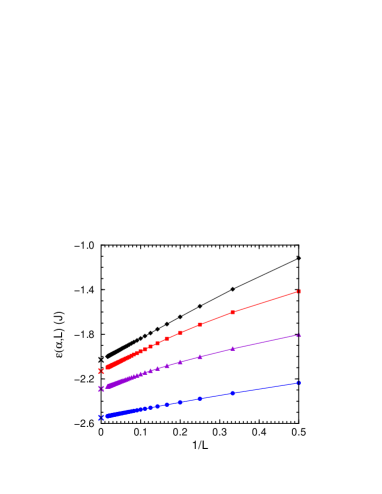
Figure 4: (Color online) Ground state energies per site $\varepsilon(\alpha,L)$ for the QIM on open chains (7) as functions of inverse chain’s length $1/L$ (for $2\leq L\leq 61$) plotted for $\alpha=1$, 3/4, 1/2 and $1/4$, from bottom to top. Linear fit gives the asymptotic values of energies for $L\to\infty$, indicated by crosses; these are: $\varepsilon(\alpha,L\to\infty)=-2.55$, $-2.29$, $-2.13$ and $-2.03$ for the respective values of $\alpha$.

We define new fermion operators $\gamma^{\dagger}_{i}$ as follows

$$\gamma^{\dagger}_{i}=\sum_{j=1}^{L}\left(\alpha_{ij}c^{\dagger}_{j}+\beta_{ij}c_{j}\right)\,,$$ (28)

for $i=1,2,\dots,L$. Coefficients $\alpha_{ij}$ and $\beta_{ij}$ can be chosen in such a way that the transformation is canonical and ${\cal H}(\alpha,L)$ takes the diagonal form:

$${\cal H}(\alpha,L)=\sum_{i=1}^{L}E_{i}(\alpha,L)\left(\gamma^{\dagger}_{i}\gamma_{i}-\frac{1}{2}\right)\,.$$ (29)

Both excitations energies $E_{i}$ and transformation coefficients $\{\alpha_{ij},\beta_{ij}\}$ can be determined from the condition

$$[{\cal H}(\alpha,L),\gamma^{\dagger}_{i}]=E_{i}\gamma^{\dagger}_{i}\,.$$ (30)

This leads to an eigenequation

$$\left(\begin{array}[]{cc}A&B\\ -B&-A\end{array}\right)\left(\begin{array}[]{c}\vec{\alpha}_{i}\\ \vec{\beta}_{i}\end{array}\right)=E_{i}\left(\begin{array}[]{c}\vec{\alpha}_{i}\\ \vec{\beta}_{i}\end{array}\right)\ ,$$ (31)

where $A$ and $B$ are matrices of size $L\times L$ ($A$ is a symmetric and $B$ is an antisymmetric matrix), and $\vec{\alpha}_{i}$, $\vec{\beta}_{i}$ are vectors of length $L$. The explicit form of $A$ and $B$ for $L=4$ is

$$A=2J\left(\begin{array}[]{cccc}-2\alpha&1&0&0\\ 1&-2\alpha&1&0\\ 0&1&-2\alpha&1\\ 0&0&1&-2\alpha\end{array}\right)$$ (32)

and

$$B=2J\left(\begin{array}[]{cccc}0&1&0&0\\ -1&0&1&0\\ 0&-1&0&1\\ 0&0&-1&0\end{array}\right)\ ,$$ (33)

which can be simply generalized to the case of any finite $L$. The spectrum of ${\cal H}(\alpha,L)$ can be now determined by a numerical diagonalization of the $2L\times 2L$ matrix from Eq. (31). For each $L$ one obtains a set of $2L$ eigenvalues symmetric around zero. Only the positive ones are the excitation energies $E_{i}$ appearing in Eq. (29). Therefore, the ground state energy $E_{0}(\alpha,L)$ is obtained in absence of any excited states, so the energy per site can be easily expressed as

$$\varepsilon(\alpha,L)=\frac{1}{L}E_{0}(\alpha,L)=-\frac{1}{2L}\;\sum_{i=1}^{L}E_{i}(\alpha,L)\ .$$ (34)

Fixing $\alpha$ and increasing $L$ we can trace the dependence of $\varepsilon(\alpha,L)$ on the system size and make an extrapolation to an infinite chain $L\to\infty$. Results for $\varepsilon(\alpha,L)$ (34) as a function of decreasing $1/L$, obtained for $\alpha=1,3/4,1/2,1/4$ and $L$ changing from $2$ to $61$, are shown in Fig. 4. The energies decrease with increasing $L$ which suggests that the ground state corresponds indeed to a closed chain without any defects, as presented in Sec. III.2.

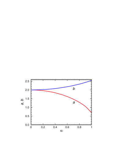
Figure 5: (Color online) Coefficients $a(\alpha)$ (lower line) and $b(\alpha)$ (upper line) of the linear fit (35) performed for the points $(1/60,\varepsilon(\alpha,60))$ and $(1/61,\varepsilon(\alpha,61))$ for different values of $\alpha$. At $\alpha=0$ one recovers the classical values of the Ising chain.

The dependence of $\varepsilon(\alpha,L)$ on $1/L$ seems to be almost linear in each case. This is almost exact for $\alpha=1$ and for $\alpha=1/4$, while it holds approximately for intermediate values of $\alpha$ for in the regime of sufficiently large $L$. This observation can be used to derive a simple, approximate formula for the energy $\varepsilon(\alpha,L)$. One can take the values of $\varepsilon(\alpha,L)$ obtained for two largest $L$ ($L=60,61$) with fixed $\alpha$ and perform a linear fit. Hence, we get

$$\varepsilon(\alpha,L)\cong a(\alpha)\,\frac{1}{L}-b(\alpha)\ ,$$ (35)

with coefficients $a$ and $b$ depending on $\alpha$. These new functions can be determined numerically for $\alpha$ changing between $0$ and $1$ with sufficiently small step. Results obtained by a numerical analysis are plotted in Fig. 5. Both $a$ and $b$ starts from a value $2$ at $\alpha=0$, then $a(\alpha)$ decreases monotonically to about $0.72$ while $b(\alpha)$ slightly increases to $2.55$ at $\alpha=1$. Eq. (35) is exact for $\alpha=0$ and any $L$, as well as for $L=60,61$ and any $\alpha$. Nevertheless, looking at Fig. 4, one can expect it to be a good approximation in case of sufficiently large $L$. From this formula one can read that for $L\to\infty$ one gets $E_{0}(\alpha,L)=-Lb(\alpha)+O(L^{0})$ which agrees with the classical intuition based on extensiveness of the internal energy.

III.5 Lowest energy excitations

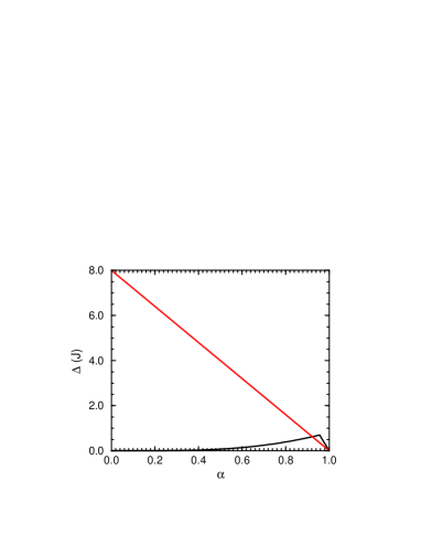
Figure 6: (Color online) Excitation energy $\Delta(J)$ as a function of $\alpha$ for: (i) a ladder with $N=4$ rungs (lower line) and (ii) an infinite ladder (upper line). In the first case, as long as the QPT is not approached, the excited state remains in the ground state subspace with $r_{i}\equiv-1$ and contains one Bogoliubov quasiparticle with $k=\pi$. Excitation energy is small, starts from zero and decreases quickly with growing $N$. The latter excited state collapses to the ground state for $N=\infty$, so the first excitation is here different than the one for infinite $N$. On the contrary, the excited state for $N=\infty$ contains two Bogoliubov quasiparticles with $k=0^{\pm}$. This leads to the linear gap following $\Delta(\alpha)=8J(1-\alpha)$.

As we pointed out in Sec. III.2, the lowest excited state in the case of a finite system, for $\alpha$ far enough from $\alpha=1$, is simply $\gamma_{\pi}^{\dagger}|0_{+}\rangle$ and belongs to the subspace $r_{i}\equiv-1$. This is a collective excitation creating a wave of spin–flips in the ground state. Close to $\alpha=1$ one finds that the lowest excited state is the ground state from the subspace $r_{i}\equiv 1$ which means that the spin order along the rungs changes from AF to FM one along the $z$–th axis.

The lowest energy excitation changes qualitatively in the thermodynamic limit $N\to\infty$, where $\gamma_{\pi}^{\dagger}|0_{+}\rangle$ and $|0_{+}\rangle$ states have the same energy and the dominating excitation is a pair of Bogoliubov quasiparticles with $k=0^{\pm}$ which corresponds to flipping one spin at $\alpha=0$. The first excited state remains in the $r_{i}\equiv-1$ subspace for all $\alpha$ and the gap follows linear law $\Delta(\alpha)=8J(1-\alpha)$, see Fig. 6. This shows that in the thermodynamic limit ($N\to\infty$) the low energy spectrum of the ladder is the same as for ordinary QIM. Note that such behavior is in sharp contrast with the case of finite ladder of $N=4$ rungs.

IV Canonical ensemble for the ladder

IV.1 Partition function

In order to construct the partition function of spin ladder (1), we shall analyze its quantum states in different subspaces. Every invariant subspace introduced in Sec. II is labelled by a string $r_{1}r_{2}\cdots r_{N}$. Let us consider an exemplary string of the form

$$1\ 1\ 1\ \bar{1}\ 1\ \bar{1}\ 1\ 1\ \bar{1}\ \bar{1}\ \bar{1}\ 1\ 1\ \bar{1}\ 1\ 1\ 1\ 1\ \bar{1}\ \bar{1}\ \bar{1}\ 1\ ,$$ (36)

where $\bar{1}=-1$, and either $r_{i}=r_{i+1}$ or $r_{i}\not=r_{i+1}$. Each time when $r_{i}=r_{i+1}$ the chain continues, and when $r_{i}\not=r_{i+1}$ we may say that a kink occurs at site $i$ in the chain. We introduce a periodic boundary condition, so the string is closed to a loop and $r_{N}$ stands next to $r_{1}$. From the point of view of the reduced Hamiltonian ${\cal H}_{r_{1}r_{2}\cdots r_{N}}$, given by Eq. (5), it is useful to split the string $\{r_{i}\}$ into chains and kinked areas. A chain is a maximal sequence of $r_{i}$’s without any kinks consisting at least of two sites. Kink areas are the intermediate areas separating neighboring chains. Using these definitions we can divide our exemplary string (36) as follows

$$1\ 1\ 1)\ \bar{1}\ 1\ \bar{1}\ (1\ 1)\ (\bar{1}\ \bar{1}\ \bar{1})\ (1\ 1)\ \bar{1}\ (1\ 1\ 1\ 1)\ (\bar{1}\ \bar{1}\ \bar{1})\ (1\ ,$$

(37)

where we adopt the convention to denote chains as $(r_{i}r_{i+1}\cdots r_{i+p})$, and kink areas as $)r_{i}r_{i+1}\cdots r_{i+q}($. For any string of $r_{i}$’s containing $m$ chains we can define chain configuration $\{L_{i}\}$ with $i=1,2,\dots,m$, where $L_{i}$’s are the lengths of these chains put in descending order. In case of our exemplary string its chain configuration is $\{4,4,3,3,2,2\}$. Variables $\{L_{i}\}$ must satisfy three conditions: (i) $L_{i}\geq 2$ for all $i$, (ii) $\sum_{i=1}^{m}L_{i}\leq N$, and (iii) $\prod_{i=1}^{m}(-1)^{L_{i}}\equiv(-1)^{m}$. The first two of them are obvious, while the last one is a consequence of the periodic boundary conditions. Using chain parameters the effective Hamiltonian ${\cal H}_{r_{1}r_{2}\cdots r_{N}}$ can be written as a sum of commuting operators

$${\cal H}_{r_{1}r_{2}\cdots r_{N}}(\alpha)=\sum_{i=1}^{m}{\cal H}(\alpha,L_{i})-2J\alpha\sum_{i=1}^{K}\tau_{i}^{x}+2JC_{\vec{r}}(\alpha)\ ,$$ (38)

where $K=N-\sum_{i=1}^{m}L_{i}$ stands for the total size of kinked areas. This formula refers to all subspaces excluding those with $r_{i+1}\equiv r_{i}$, where we have already obtained exact solutions. The evaluation of the constant $C_{\vec{r}}(\alpha)$ can be completed by considering chain and kink areas in each subspace, see appendix. Having the diagonal form of ${\cal H}(\alpha,L)$, given by Eq. (29), one can now calculate partition function for the ladder of $2N$ spins. It can be written as follows

$${\cal Z}(\alpha) = \sum_{\{L_{i}\}}\sum_{R_{\{L_{i}\}}}F_{\alpha}[\{L_{i}\},R_{\{L_{i}\}}]e^{-2JC_{\vec{r}}/T}Z(\alpha,\{L_{i}\})$$ (39)

$$+ Z_{0}(\alpha)\ ,$$

where the sum over all $\{\vec{r}\}$ subspaces is replaced by sums over all chain configurations $\{L_{i}\}$ and all $R=\sum_{i=1}^{N}r_{i}$ configurations possible for a given $\{L_{i}\}$. Factor $F_{\alpha}[\{L_{i}\},R_{\{L_{i}\}}]$ is a number of $\vec{r}$ subspaces for fixed chain configuration and fixed $R$ when $\alpha<1$, and for $\alpha=1$ it is a number of $\vec{r}$ subspaces when only $\{L_{i}\}$ is fixed. Partition function for any subspace containing open QIM chains or kinked areas is given by

$$Z(\alpha,\{L_{i}\}) = 2^{N}\cosh^{K}\left[\frac{2J}{T\alpha}\right]$$ (40)

$$\times \prod_{i=1}^{n}\prod_{j=1}^{l_{i}}\,\cosh^{N(l_{i})}\left[\frac{E_{j}(\alpha,l_{i})}{2T}\right]\ ,$$

where $\{l_{i}\}$ ($i=1,2,\dots,n$) are the different lengths of the chains appearing in the chain configuration $\{L_{i}\}$, $N(l_{i})$ stands for the number of chains of the length $l_{i}$, and $T$ is temperature in units of $k_{B}=1$. For example, the chain configuration $\{4,4,3,3,2,2\}$ of Eq. (37) has $n=3$, $\{l_{i}\}=\{4,3,2\}$ and $N(l_{i})\equiv 2$. The term $Z_{0}(\alpha)$ is a contribution from subspaces with $r_{i+1}\equiv r_{i}$. Using exact solutions (18), available in these subspaces, one finds that

$$\!\!Z_{0}(\alpha)\! = \cosh\left[\frac{2J}{T}N(1-\alpha)\right]$$ (41)

$$\times \!\!\sum_{S=\pm 1}\!\left(\prod_{q=0}^{N-1}\!\cosh\frac{E_{q}^{S}}{T}+S\prod_{q=0}^{N-1}\!\sinh\frac{E_{q}^{S}}{T}\right),$$

where the quasiparticle energies are:

$$E_{q}^{+}\! = 2J\left\{1+\alpha^{2}+2\alpha\cos\left(\frac{2q+1}{N}\pi\right)\right\}^{1/2},$$ (42)

$$E_{q}^{-}\! = 2J\left\{1+\alpha^{2}+2\alpha\cos\left(\frac{2q+2}{N}\pi\right)\right\}^{1/2}.$$ (43)

Appearance of both sine and cosine hyperbolic functions in $Z_{0}$ (41) is due to the projection operators ${\cal P}$ introduced in section III.1.

IV.2 Combinatorial factor

To obtain numerical values of the partition function one has to get the explicit form of the combinatorial factor $F_{\alpha}[\{L_{i}\},R_{\{L_{i}\}}]$. This can be done in a simple way only for $\alpha=1$ when $C_{\vec{r}}(\alpha)=0$, see Eq. (6). Then we have

$$F_{\alpha=1}[\{L_{i}\},R_{\{L_{i}\}}]\equiv F_{1}[\{L_{i}\}]\ ,$$ (44)

where $F_{1}[\{L_{i}\}]$ is the number of different $\vec{r}$ subspaces that can be obtained from a fixed chain configuration $\{L_{i}\}$. Now we can derive a formula for this combinatorial factor.

The chains can be put into the $r_{i}$ string in any order and these of equal length are indistinguishable. Apart from chains, there are also $r_{i}$’s belonging to the kinked areas which determine the actual string configuration. We have $K=N-\sum_{i=1}^{m}L_{i}$ of them, they are indistinguishable and can be distributed among $m$ kinked areas. These degrees of freedom lead to a combinatorial factor

$$\frac{m!}{N(l_{1})!\dots N(l_{n})!}\left(\begin{array}[]{c}K+m-1\\ K\end{array}\right),$$ (45)

where $l_{1},l_{2},\dots,l_{n}$ $(n\leq m)$ are the lengths of the chains without repetitions and $N(l_{i})$ is a number of chains of the length $l_{i}$. After determining the length of the first chain $L_{1}$ and the size of its kink area $A_{1}$, we still need to fix the position of $r_{1}$. We have exactly $L_{1}+A_{1}$ possibilities. Next, we have to sum up over all possible values of $L_{1}$ (which are $l_{1},l_{2},\dots,l_{n}$), all possible sizes of the kink area $A_{1}$ (which are $1,2,\dots,K$) and multiply by a combinatorial factor (45) calculated for the remaining part of the string. The result is

$$F_{1}[\{L_{i}\}] = 2\sum_{i=1}^{n}N(l_{i})\frac{(m-1)!}{N(l_{1})!\dots N(l_{n})!}$$ (48)

$$\times \!\sum_{a=0}^{K}\;(l_{i}+a)\left(\begin{array}[]{c}K-a+m-2\\ K-a\end{array}\right),$$

where the factor of $2$ in front comes from the fact that $r_{1}=\pm 1$. This number tells us how many times a given energy spectrum repeats itself among all subspaces when $\alpha=1$. The binomial factor appearing in formula (48) needs to be generalized with $\Gamma$ functions when $m=1$.

V COMPASS ladder at finite temperature

V.1 Correlation functions and chain fragmentation

Nearest-neighbor correlation functions can be easily derived at finite temperature from the partition function ${\cal Z}(\alpha,\beta,\gamma)$, if we substitute our initial Hamiltonian ${\cal H}(\alpha)$ given by Eq. (1) by

$${\cal H}(\alpha,\beta,\gamma) = 2J\sum_{i=1}^{N}\left\{\gamma\sigma^{x}_{2i-1}\sigma^{x}_{2i}+(1-\alpha)\sigma^{z}_{2i-1}\sigma^{z}_{2i}\right\}$$ (49)

$$+ J\beta\sum_{i=1}^{N}\left(\sigma^{z}_{2i-1}\sigma^{z}_{2i+1}+\sigma^{z}_{2i}\sigma^{z}_{2i+2}\right)\,.$$

Then, after calculating the partition function, we recover spin correlations by differentiating ${\cal Z}(\alpha,\beta,\gamma)$ with respect to $\beta$ and $\gamma$, and inserting $\gamma=\alpha$ and $\beta=1$ to the obtained correlations to derive the final results. Once again, this can be done in a simple way for small ladders. Correlation functions $\langle\sigma_{2i-1}^{x}\sigma_{2i}^{x}\rangle$ and $\langle\sigma_{2i-1}^{z}\sigma_{2i+1}^{z}\rangle$ for spin ladder (1) at $\alpha=1$ (quantum compass ladder) are shown in Fig. 7 for increasing temperature $T$. Other nearest neighbor correlations vanish at $\alpha=1$ for trivial reasons.

Fig. 7 shows the qualitative difference between correlation functions of spin ladder (1) and those of periodic QIM chain (8) of length $N$, that appears in the ground subspaces $r_{i}\equiv r_{i+1}$. When all the subspaces are considered, thermal fluctuations gradually destroy the spin order along the legs and the $\langle\sigma_{2i-1}^{z}\sigma_{2i+1}^{z}\rangle$ correlations weaken. On the contrary, the $\langle\sigma_{2i-1}^{x}\sigma_{2i}^{x}\rangle$ correlations on the rungs are robust in the entire range of physically interesting temperatures $0<T<2J$, as the ZZ interactions destroying them are gradually suppressed with increasing $T$ due to the increasing size of kinked areas.

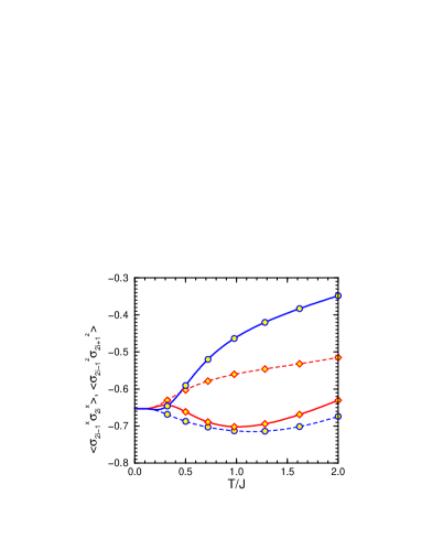
Figure 7: (Color online) Nearest neighbor correlation functions, $\langle\sigma_{2i-1}^{x}\sigma_{2i}^{x}\rangle$ on the rungs (diamonds and red lines) and $\langle\sigma_{2i-1}^{z}\sigma_{2i+1}^{z}\rangle$ along the ladder legs (circles and blue lines), calculated for the compass ladder ($\alpha=1$) of $2N=8$ spins for increasing temperature $T$, taking into account: ($i$) all subspaces (solid lines) for increasing temperature $T$, and ($ii$) only the subspace which contains the ground state $r_{i}\equiv-1$ (dashed lines).

The above result is qualitatively different from the QIM results shown by dashed lines in Fig. 7, where thermal fluctuations initially increase intersite correlations of $z$–th spin components along the ladder legs and reduce the influence of the transverse field acting on $\tau_{i}^{x}$ pseudospins due to spin interactions $2J\sigma_{2i-1}^{x}\sigma_{2i}^{x}$ on the rungs. In the latter case thermal fluctuation in certain interval of temperature can enhance local spin ZZ correlations along the ladder legs at the cost of disorder in the direction of external field. This is because pseudospin interaction involves $\tau^{z}_{i}$ operators, not $\tau^{x}_{i}$ ones. Remarkably, in the full space, see solid lines in Fig. 7, the spin correlations are initially the same (at low $T$) as those for the QIM, but this changes when temperature $T\simeq 0.3J$ is reached and the two curves cross — then the rung correlations start to dominate. The crossing is caused by the growth of the kinked areas, as shown in Fig. 8, which are free of quantum fluctuations and therefore favor rung correlations of $x$–th spin components.

Another interesting information on excitations in the quantum compass ladder is the evolution of the average chain configuration with increasing temperature. As we know from Sec. IV.1, every subspace can be characterized by the lengths of chains that appear in its $r_{i}$ label. Chain configurations can in turn be characterized by: ($i$) the number of chains which are separated by kinks $m$, and ($ii$) the total size of kinked areas $K$. Thermodynamic averages of both quantities, $\langle m\rangle$ and $\langle K\rangle$, can be easily determined at $\alpha=1$ even for a relatively large system using the combinatorial factor $F_{1}[\{L_{i}\}]$ (48) calculated in Sec. IV.2. In the limit of $T\to\infty$ one has:

$$\langle m\rangle_{\infty} = \frac{\sum_{\{L_{i}\}}F_{1}[\{L_{i}\}]\left(N-\sum_{j=1}^{m}L_{j}\right)}{\sum_{\{L_{i}\}}F_{1}[\{L_{i}\}]}\,,$$ (50)

$$\langle K\rangle_{\infty} = \frac{\sum_{\{L_{i}\}}F_{1}[\{L_{i}\}]m[\{L_{i}\}]}{\sum_{\{L_{i}\}}F_{1}[\{L_{i}\}]}\,,$$ (51)

where $m[\{L_{i}\}]$ is the number of $\{L_{i}\}$ in the chain configuration $L_{1},L_{2},\cdots,L_{m}$.

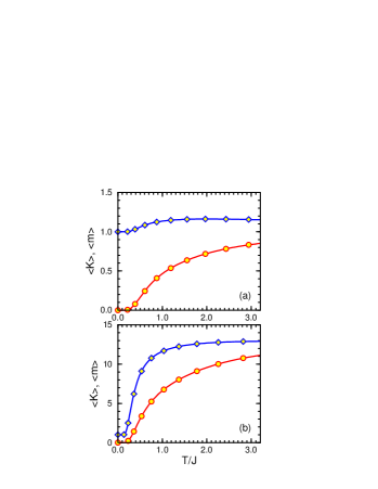
Figure 8: (Color online) Average size of the kinked areas $\langle K\rangle$ (51) (circles and red lines) and the average number of chains $\langle m\rangle$ (50) (diamonds and blue lines) for the quantum compass ladder (1) (at $\alpha=1$) consisting of: (a) $2N=8$, and (b) $2N=104$ spins. The mean size of kinked areas $\langle K\rangle$ increases monotonically with increasing temperature $T$ to the asymptotic value $N/4$, see Eq. (52). The average number of chains $\langle m\rangle$ behaves differently, growing quickly to a maximal value at intermediate $T$ and then decreasing slowly when $T\to\infty$ towards: (a) $1.125$, and (b) $13+12\times 10^{-15}$.

In Fig. 8 we show the average quantities $\langle m\rangle$ and $\langle K\rangle$ for ladders of $2N=8$ (left) and $2N=104$ spins (right). In both cases the average number of chains $\langle m\rangle$ starts from $1$ and the average size of the kinked areas $\langle K\rangle$ starts from $0$, corresponding to a single chain without kinks in the ground state at $T=0$. The number of chains $\langle m\rangle$ grows to a broad maximum in the intermediate temperature range and decreases asymptotically to a finite value. This non–monotonic behavior is due to the fact that the states with the highest energy, which become accessible when $T\to\infty$, do not belong to the subspaces with large number of chains. The mean value of kinks $\langle K\rangle$ follows $\langle m\rangle$ but increases monotonically in the entire range of $T$, and for finite $T$ one finds that $\langle K\rangle<\langle m\rangle$. By looking at the current results one may deduce that in case of $T\to\infty$ and for large $N\gg 1$ both quantities approach

$$\langle m\rangle_{\infty}=\langle K\rangle_{\infty}=\frac{N}{4}\,.$$ (52)

This is an interesting combinatorial feature of the chain configurations which is not obvious when we look at the explicit form of the combinatorial factor $F_{1}[\{L_{i}\}]$ (48). Note that Eq. (52) gives an integer due to our choice of system sizes $2N$ considered here, being multiplicities of 8, i.e., $N$ is a multiplicity of 4.

V.2 Spectrum of a large system

The combinatorial factor $F_{1}[\{L_{i}\}]$ given by Eq. (48) enables us to calculate the partition function ${\cal Z}(1)$ (39) for a large system when $\alpha=1$. As a representative example we consider a ladder consisting of $2N=104$ spins. Even though we can reduce Hamiltonian (1) to a diagonal form when $2N=104$, as shown in previous paragraphs, it is still impossible to generate the full energy spectrum for practical reasons — simply because the number of eigenstates is too large. Instead, we can obtain the density of states in case of $\alpha=1$ using the known form of the partition function (39) and of the combinatorial factor (48). Partition function for imaginary $1/T$ can be written as

$${\cal Z}(ix)=\sum_{p=0}^{4^{N}-1}e^{-ixE_{p}}=\int_{E_{0}-\varepsilon}^{-E_{0}+\varepsilon}dEe^{-ixE}\rho(E)\ ,$$ (53)

where

$$\rho(E)\equiv\sum_{p=0}^{4^{N}-1}\delta(E-E_{p})\ ,$$ (54)

and where sum is over all eigenenergies $E_{p}$ of the ladder. Parameter $E_{0}$ is the energy of the ground state. Small and positive $\varepsilon$ is introduced to formally include $\pm E_{0}$ into integration interval. Here we used the fact that ladder’s spectrum is symmetric around zero at the compass point $\alpha=1$ (see Fig. 2). Function $\rho(E)$ can be easily recognized as the density of states.

Using $x=2\pi n/w$ in Eq. (53), with $w=2(|E_{0}|+\varepsilon)$ standing for the length of the integration interval and $n$ being integer, we easily recover the density of states $\rho(E)$ (54) in a form of the Fourier cosine expansion

$$\rho(E)=\frac{2}{w}\sum_{n=1}^{\infty}{\cal Z}\left(2i\pi\frac{n}{w}\right)\cos\left(2\pi\frac{n}{w}E\right)+\frac{1}{w}{\cal Z}(0)\ ,$$ (55)

with amplitudes given by the partition function ${\cal Z}(ix)$.

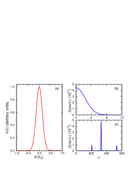
Figure 9: (Color online) Relative density of states $N(E)$ (a) as a function of energy ratio $E/E_{0}$ and Fourier coefficients ${\cal Z}\left(2i\pi\frac{n}{w}\right)$ as functions of $n$ for $0\leq n\leq 12$ (b) and for $13\leq n\leq 600$ (c) calculated for the ladder of $2N=104$ spins. Relative density of states reminds a gaussian centered in zero with the width being roughly $0.15$ of the spectrum width $w$. This follows from the gaussian behavior of ${\cal Z}\left(i2\pi\frac{n}{w}\right)$ coefficients for small $n$ (panel (b)). Plot (c) reveals peaks in ${\cal Z}\left(i2\pi\frac{n}{w}\right)$ for $n=208,330,533$, three order of magnitude weaker than for $n=0$, corresponding with periodic condensations of the energy levels every $\Delta E=1.28,0.81,0.50J$ (especially every $0.81J$).

In practice we cannot execute the sum above up to infinity. Therefore, it is convenient to define $\rho_{c}(E)$ which is given by the same Eq. (55) as $\rho(E)$ but where the sum has a cutoff for $n=c$. The heights of peaks in $\rho_{c}(E)$ are expected to grow in an unlimited way with increasing value of $c$, so it is convenient to define the normalized density of states $N(E)$ as

$$N(E)=\rho_{c}(E)/\rho_{c}(0)\ .$$ (56)

The results for the compass ladder ($\alpha=1$) of $2N=104$ spins are shown in Fig. 9. These are relative density of states $N(E)$ for cutoff $c=600$ and Fourier coefficients ${\cal Z}\left(2i\pi\frac{n}{w}\right)$ for two intervals of $n$. Results obtained for lower cutoffs show that the overall gaussian shape of $N(E)$, shown in Fig. 9(a), does not change visibly if only $c>8$. This allows us to conclude that the spectrum of the compass ladder becomes continuous when the size of the systems increases which is not the case for the Ising ladder ($\alpha=0$). Higher values of $n$ are investigated to search for more subtle effects than gaussian behavior of $N(E)$. These are found by looking at the amplitudes ${\cal Z}\left(2i\pi\frac{n}{w}\right)$ in high $n$ regime [Fig. 9(c)], as the low $n$ regime [Fig. 9(b)] encodes only the gaussian characteristic of the spectrum. One finds three sharp maxima of the amplitudes for $n=208,330,533$ out of which the one with $n=330$ is about five times more intense than the rest, but it is still $10^{3}$ times weaker than the peak in $n=0$. These values of $n$ correspond with some periodic condensations of the energy levels with periods $\Delta E=1.28,0.81,0.50J$ respectively which are visible in $N(E)$ only in vicinity of $E=\pm E_{0}$.

VI Heat capacity

VI.1 From Ising to compass model

In this Section we analyze heat capacity to identify characteristic excitation energies in the compass ladder. We begin with complete results for the ladder consisting of $2N=8$ spins shown in Fig. 1, where all chain configurations can be written explicitly. Using Eq. (39) for the partition function, one can next calculate all thermodynamic functions including average internal energy and the heat capacity.

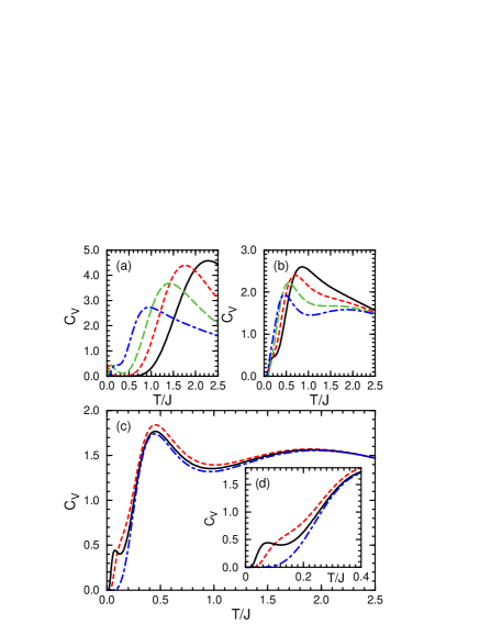
Figure 10: (Color online) Heat capacities $C_{V}$ for spin ladder (1) of $2N=8$ spins, shown in Fig. 1, with parameter $\alpha$ equal to: (a) $\alpha=0,0.49,0.69,0.85$, (b) $\alpha=0.87,0.90,0.94,0.97$, and (c) $\alpha=0.982,0.988,1$. In panels (a) and (b) lines from right to the left (solid, dashed, long-dashed, dashed-dotted) correspond with growing $\alpha$. In panels (c) and (d) the values of $C_{V}$ for $\alpha=0.982,0.988,1$ are shown by dashed, solid and dashed-dotted lines, respectively. Panel (d) shows the low temperature data of panel (c) (for $\alpha>0.98$), with a well developed small peak at low temperature originating from the critical excitations between subspaces $r_{i}\equiv 1$ and $r_{i}\equiv-1$ close to $\alpha=1$; it disappears at $\alpha=1$.

Results for the heat capacity $C_{V}$ for different values of $\alpha$ are shown in Fig. 10. These plots cover three characteristic intervals of $\alpha$ where the behavior of curves changes qualitatively by appearance or disappearance of certain maxima. The positions of these maxima correspond to possible excitation energy scales of the system that change at increasing $\alpha$ and their intensities reflect the number of possible excitations in a given energy interval. In case of $\alpha=0$ [Fig. 10(a)], we see a single maximum at $\sim 2.2J$ which corresponds to flipping spins in an Ising spin ladder. Switching on the XX interactions and weakening the ZZ interactions on the rungs has two effects: ($i$) decreasing energy and intensities of the high–energy maximum, and ($ii$) appearance of a low–energy mode in every subspace with QIM chains which manifests itself as a peak with low intensity at low temperature $T$, see Fig. 10(a). At $\alpha\simeq 0.85$ this mode overlaps with modes of higher energies and until $\alpha\simeq 0.94$ there is a single peak again with a shoulder at high values of $T$, shown in Fig. 10(b). Then the excitation energies separate again and a broad peak appears for high $T$ accompanied by a distinct maximum at $T\simeq 0.4J$.

In Fig. 10 we recognize the characteristic features for the QIM chains present in most of the subspaces which are influenced by the excitations mixing different subspaces. If we had only one subspace with $r_{i}\equiv-1$, i.e., the one containing the ground state, then we would have two maxima in $C_{V}$ for all $0\leq\alpha\leq 1$ — one of low intensity in the regime of low temperature $T$, and another one in high $T$, broad and intense. The small maximum corresponds with low–energy mode of QIM that disappears for certain $\alpha>1$. This is not the case for other subspaces where QIM chains are fragmented and kinked area are formed. In case of the $1\bar{1}\bar{1}\bar{1}$ subspace the low–energy peak in $C_{V}$ vanishes at $\alpha\simeq 0.65$ and the high-energy peak persists and moves to higher temperatures with the increase of $\alpha$. The situation is similar for the $11\bar{1}\bar{1}$ subspace but the peak disappears at $\alpha\simeq 0.75$ and in the classical subspace $1\bar{1}1\bar{1}$ we have only one maximum for any $\alpha$. One can deduce now that the general rule is that the separation of peaks in heat capacity is reduced primarily by the growth of kinked areas and secondarily by the fragmentation of chains. This separation of energy scales is also visible in Fig. 2 where the spectra in different subspaces are shown; below certain $\alpha$ in all cases but (d), which is the classical subspace, the energy gap between the ground state and first excited state is smaller than other energy gaps appearing in the subspace.

The mixing of different subspaces in the partition function makes the peaks in $C_{V}$ overlap which can result in reducing their number. This happens in Fig. 10(b); for solid ($\alpha=0.87$) and dashed ($\alpha=0.90$) curve we have only one maximum. For higher or lower $\alpha$ the energy scales remain separated which is due to fact that: ($i$) soft modes survive in most of subspaces for low $\alpha$, and ($ii$) for high $\alpha$ the high–energy modes become even tougher and do not overlap with soft modes still present in subspaces with small kinked areas. The last phenomenon characteristic for the ladder are excitations between $r_{i}\equiv-1$ and $r_{i}\equiv 1$ subspace in the vicinity of the QPT. This yields to the appearance of the new energy scale $\Delta(\alpha)=4NJ(1-\alpha)$ at $\alpha\simeq 0.987$ which manifests itself as a small peak in heat capacity in low temperature. This maximum vanishes at $\alpha=1$, as shown in Fig. 10(d).

VI.2 Generic features at large N

After understanding the heat capacity in a small system of $N=8$ spin (Sec. VI.1), we analyze a large system using the statistical analysis of Sec. VI. Obtaining combinatorial factor $F_{\alpha}[\{L_{i}\},R_{\{L_{i}\}}]$ in case of $\alpha<1$ is difficult and likely even impossible in a general way without fixing $N$. Hence we focus on the compass ladder ($\alpha=1$) For the compass ladder of $2N=104$ spins considered in Sec. V.2, one finds $2^{52}$ invariant subspaces. Although the eigenvalues can be found in each subspace, it is not possible to sum up over all subspaces for practical reasons and a statistical analysis is necessary. Therefore, the knowledge of the combinatorial factor $F_{1}[\{L_{i}\}]$, see Eq. (48), is crucial to calculate partition function ${\cal Z}(1)$ (39). Fortunately, knowing it we only need to consider different chain configurations which are not very numerous — there are only $140854$ of them. This means that on average each energy spectrum of the effective Hamiltonian repeats itself almost $32\times 10^{9}$ times throughout all subspaces.

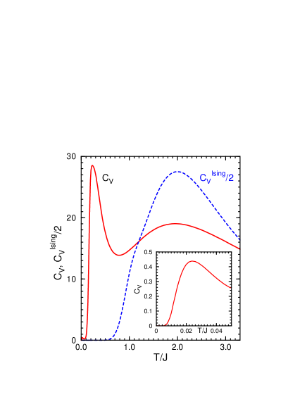
Figure 11: (Color online) Heat capacity $C_{V}$ for the compass ladder of $2N=104$ spins (spin ladder (1) at $\alpha=1$, solid line) as a function of temperature $T$ . The main difference with the case of $2N=8$ spins [see Fig. 10(c)] is a small maximum appearing at very low $T\simeq 0.02J$, see inset. This peak originates from the low–energy modes in subspaces $r_{i}\equiv r_{i+1}$ which exist in sufficiently long chains described by the QIM. Dashed line show heat capacity of the Ising ladder ($\alpha=0$) of the same size.

The statistical analysis of the compass ladder consisting of $2N=104$ spins in terms of: ($i$) mean values of kinked areas $\langle K\rangle$ (51), and ($ii$) the number of chains $\langle m\rangle$ (50), was already presented in Fig. 8(b), while the energy spectrum was discussed in Sec. V.2. Here we present the heat capacity $C_{V}$ for the compass ladder of this size in Fig. 11. At high temperature one finds a broad maximum centered at $T\simeq 2J$ which originates from dense excitation spectrum at the compass point ($\alpha=1$), cf. the spectrum of the compass ladder with $2N=8$ spins shown in Fig. 2. We remark that the broad maximum of Fig. 11 has some similarity to broad maxima found in the specific heat (heat capacity) of spin glasses.Geo01 However, here the broad maximum in the heat capacity does not originate from disorder but solely indicates frustration, similar as in some other models with frustrated spin interactions.Bec03 We emphasize that the present results could be obtained only by developing a combinatorial analysis of a very large number of possible configurations of spin ladder, and due to the vanishing constant $C_{\vec{r}}(\alpha=1)=0$ (6) in the energy spectrum for the compass ladder. Unfortunately, the present problem is rather complex due to the quantum nature of spin interactions, but in case of the binomial 2D Ising spin glass an exact algorithm to compute the degeneracies of the excited states could be developed recently.Ati08

The heat capacity $C_{V}$ of Fig. 11 at low temperature is qualitatively similar to the one obtained for $2N=8$ spins, see Fig. 10(c), but the steep maximum at low $T$ is here moved to lower temperature $T\simeq 0.2J$. We also identified an additional (third) peak in the regime of rather low temperature $T\simeq 0.02J$ (shown in the inset). This maximum originates from the QIM (8) where the energies of the ground state and of the first excited state approach each other for increasing $N$, if only $\alpha\leq 1$. Thus, this lowest peak in the heat capacity obtained for the compass ladder of $2N=104$ spins has to be considered as a finite size effect — for increasing system size it is shifted to to still lower temperature $T$, and would disappear in the thermodynamic limit $N\to\infty$, in agreement with the qualitative change of low energy spectrum of the QIM.

VII Summary and conclusions

We have investigated an intriguing case of increasing frustration in a spin ladder (1) which interpolates between the (classical) Ising ladder and the frustrated compass ladder when the parameter $\alpha$ increases from $\alpha=0$ to $\alpha=1$. The ground state of the ladder was solved exactly in the entire parameter range by mapping to the QIM, and we verified that frustrated interactions on a spin ladder generate a QPT at $\alpha=1$, when conflicting interactions ZZ along the ladder legs compete with 2XX ones along the rungs. At this point the spin correlations on the rungs $\langle\sigma^{z}_{2i-1}\sigma^{z}_{2i}\rangle=-1$ collapses to zero and the ground state becomes disordered. We have shown that the ground state of a finite ladder has then degeneracy 2, while the analysis of the energy spectra for increasing size suggests that the degeneracy increases to 4 in the thermodynamic limit. We note that this result agrees with degeneracy $2\times 2^{L}$ found for the 2D compass model,Mil05 where $L$ is a linear dimension (the number of bonds along one lattice direction) of an $L\times L$ cluster in the 2D system. In our case of a $2\times N$ ladder, $L=1$ for ladder rungs, so indeed the degeneracy is $2\times 2=4$.

The present method of solving the energy spectrum in different subspaces separately elucidates the origin of the QPT found in the present spin ladder (1) at the point $\alpha=1$, corresponding to the frustrated interactions in the compass ladder. We argue that this approach could help to find exact solutions in a class of quasi-1D models with frustrated spin interactions, but in some cases only the ground state and not the full spectrum can be rigorously determined. For instance, this applies to a spin ladder with frustrated spin interactions between different triplet components on the rungs,Brz08 where a different type of a QPT was found recently.

By performing a statistical analysis of different possible configurations of spin ladder (1) with periodic boundary conditions we derived a partition function ${\cal Z}(\alpha)$ for a mesoscopic system of 104 spins. The calculation involves the classification of ladder subspaces into classes of chain configurations $\{L_{i}\}$ equivalent by symmetry operations and the determination of the combinatorial factor $F_{\alpha}[\{L_{i}\},R_{\{L_{i}\}}]$. We have shown that this factor can be easily determined at the compass point ($\alpha=1$), so the heat capacity of such a mesoscopic compass ladder could be found.

Summarizing, we demonstrated that spin ladder studied in this paper exhibits a QPT from a classical ordered to a quantum disordered ground state which occurs due to the level crossing, and is therefore of first order. It leads to a discontinuous change of spin correlations on the rungs when the interactions along the ladder legs and on the rungs become frustrated. Fortunately, the subspaces which are relevant for the QPT in the compass ladder considered here can be analyzed rigorously, which gives both the energy spectra and spin correlation functions by mapping the ladder on the quantum Ising model. The partition function derived in this work made it possible to identify the characteristic scales of excitation energies by evaluating the heat capacity for a mesoscopic system.

Note added in proof. After this paper was accepted, we learned about a powerful algebraic method to analyze exactly solvable spin Hamiltonians.Nus09 The present quantum compass laddeed could be also analyzed using this approach.

Appendix A Evaluation of the energy origin $C_{\vec{r}}(\alpha)$ in invariant subspaces

We need to express $\sum_{i=1}^{N}r_{i}$, which appears in $C_{\vec{r}}(\alpha)$, see Eq. (6), in terms of chain configurations $\{L_{i}\}$. This task may be accomplished by the following construction. Let us imagine certain string of $r_{i}$’s written in terms of chains $\{L_{i}\}$ and kink areas $\{A_{i}\}$:

$$A_{1}(L_{1})A_{2}(L_{2})A_{3}(L_{3})\cdots A_{k}(L_{k})\ .$$

First, we want to calculate the sum of $r_{i}$’s included in chains. We choose any $r_{i}$ from the chain $L_{1}$ and fix its sign as $r_{\rm in}$. Now this chain gives $r_{\rm in}L_{1}$ contribution to the total sum of $r_{i}$’s. To get to the second chain we have to pass through the first kink area $A_{1}$. If the number of kinks in $A_{1}$ is even, then the next chain will give the contribution $r_{\rm in}L_{2}$, and if not, then it will give the opposite number. Therefore, after passing through the whole system we will get the term

$$r_{\rm in}(L_{1}+p_{2}L_{2}+p_{2}p_{3}L_{3}+\dots+p_{2}p_{3}\dots p_{k}L_{k})\ ,$$ (57)

where $p_{i}=(-1)^{K_{i}}$, and $K_{i}$ is a number of kinks in kink area $i$. It is clear that the parameters $\{p_{i}\}$ satisfy $\prod_{i=1}^{k}p_{i}\equiv 1$. Now we need to calculate the sum of $r_{i}$’s placed in kink areas. The sign of the first chain is already chosen as $r_{\rm in}$ so we pass to $A_{2}$. For even number of kinks in $A_{2}$ the contribution is zero. If the number is odd, then we get the sum equal $-r_{\rm in}$. Passing to the next kink area we follow the same rules but we have to change $r_{\rm in}$ into $p_{2}r_{\rm in}$. The total contribution from the kink areas is then equal to

$$-p_{1}r_{\rm in}\left\{\frac{1+p_{1}}{2}+\sum_{i=2}^{k}p_{1}p_{2}\dots p_{i-1}\frac{1+p_{i}}{2}\right\}\ .$$ (58)

Using the results given in Eqs. (57) and (58) we obtain finally

$$\sum_{i=1}^{N}r_{i}=r_{\rm in}\left\{L_{1}-1+\sum_{i=2}^{k}p_{2}p_{3}\dots p_{i}(L_{i}-1)\right\}\ .$$ (59)

Thanks to this result, we can write the energy given by Eq. (38) in terms of new variables $\{L_{i},p_{i}\}$ instead of $\{r_{i}\}$ which are definitely more natural for the present problem.

References

- (1) E. Dagotto, Rep. Prog. Phys. 62, 1525 (1999).
- (2) S. Gopalan, T. M. Rice, and M. Sigrist, Phys. Rev. B49, 8901 (1994).
- (3) S. Trebst, H. Monien, C. J. Hamer, Z. Weihong, and R. P. Singh, Phys. Rev. Lett. 85, 4373 (2000).
- (4) C. Knetter, K. P. Schmidt, M. Grüninger, and G. S. Uhrig, Phys. Rev. Lett. 87, 167204 (2001).
- (5) P. Horsch and F. Mack, Eur. Phys. J. B 5, 367 (1998).
- (6) T. Vuletić, B. Korin-Hamzić, S. Tomić, B. Gorshunov, P. Haas, T. Room, M. Dressel, J. Akimitsu, T. Sasaki, and T. Nagata, Phys. Rev. Lett. 90, 257002 (2003); A. Rusydi, M. Berciu, P. Abbamonte, S. Smadici, H. Eisaki, Y. Fujimaki, S. Uchida, M. Rübhausen, and G. A. Sawatzky, Phys. Rev. B75, 104510 (2007); K. Wohlfeld, A. M. Oleś, and G. A. Sawatzky, ibid. 75, 180501(R) (2007).
- (7) S. Notbohm, P. Ribeiro, B. Lake, B. A. Tennant, K. P. Schmidt, G. S. Uhrig, C. Hess, R. Klingeler, G. Behr, B. Büchner, M. Reehuis, R. I. Bewley, C. D. Frost, P. Manuel, and R. S. Eccleston, Phys. Rev. Lett. 98, 027403 (2007).
- (8) K. Penc, J.-B. Fouet, S. Miyahara, O. Tchernyshyov, and F. Mila, Phys. Rev. Lett. 99, 117201 (2007).
- (9) L. Longa and A. M. Oleś, J. Phys. A: Math. Gen. 13, 1031 (1980).
- (10) W. Brzezicki, J. Dziarmaga, and A. M. Oleś, Phys. Rev. B75, 134415 (2007).
- (11) L. F. Feiner, A. M. Oleś, and J. Zaanen, Phys. Rev. Lett. 78, 2799 (1997).
- (12) G. Khaliullin and V. Oudovenko, Phys. Rev. B56, R14243 (1997); L. F. Feiner, A. M. Oleś, and J. Zaanen, J. Phys.: Condens. Matter 10, L555 (1998).
- (13) S. Di Matteo, G. Jackeli, C. Lacroix, and N. B. Perkins, Phys. Rev. Lett. 93, 077208 (2004); S. Di Matteo, G. Jackeli, and N. B. Perkins, Phys. Rev. B72, 024431 (2005); F. Vernay, K. Penc, P. Fazekas, and F. Mila, ibid. 70, 014428 (2004); F. Vernay, A. Ralko, F. Becca, and F. Mila, ibid. 74, 054402 (2006); G. Jackeli and D. I. Khomskii, Phys. Rev. Lett. 100, 147203 (2008).
- (14) G. Khaliullin and S. Maekawa, Phys. Rev. Lett. 85, 3950 (2000); G. Khaliullin, Prog. Theor. Phys. Suppl. 160, 155 (2005).
- (15) S. Ishihara, M. Yamanaka, and N. Nagaosa, Phys. Rev. B56, 686 (1997); L. F. Feiner and A. M. Oleś, ibid. 71, 144422 (2005).
- (16) A. M. Oleś, P. Horsch, L. F. Feiner, and G. Khaliullin, Phys. Rev. Lett. 96, 147205 (2006).
- (17) J. Zaanen, A. M. Oleś, and P. Horsch, Phys. Rev. B46, 5798 (1992); J. Zaanen and A. M. Oleś, ibid. 48, 7197 (1993); J. van den Brink, P. Horsch, and A. M. Oleś, Phys. Rev. Lett. 85, 5174 (2000); M. Daghofer, K. Wohlfeld, A. M. Oleś, E. Arrigoni, and P. Horsch, ibid. 100, 066403 (2008); K. Wohlfeld, M. Daghofer, A. M. Oleś, and P. Horsch, Phys. Rev. B78, 214423 (2008).
- (18) J. van den Brink, New J. Phys. 6, 201 (2004).
- (19) D. I. Khomskii and M. V. Mostovoy, J. Phys. A: Math. Gen. 36, 9197 (2003).
- (20) J. Dorier, F. Becca, and F. Mila, Phys. Rev. B72, 024448 (2005).
- (21) S. Wenzel and W. Janke, Phys. Rev. B78, 064402 (2008); R. Orús, A. C. Doherty, and G. Vidal, Phys. Rev. Lett. 102, 077203 (2009).
- (22) H.-D. Chen, C. Fang, J. Hu, and H. Yao, Phys. Rev. B75, 144401 (2007); Z. Nussinov and R. Ortiz, Europhys. Lett. 84, 36005 (2008).
- (23) W.-L. You and G.-S. Tian, Phys. Rev. B78, 184406 (2008).
- (24) J. H. H. Perk, H. W. Capel, M. J. Zuilhof, and T. J. Siskens, Physica A 81, 319 (1975).
- (25) E. Eriksson and H. Johannesson, Phys. Rev. B79, 224424 (2009).
- (26) V. J. Emery and C. Noguera, Phys. Rev. Lett. 60, 631 (1988).
- (27) S. Lal and M. S. Laad, J. Phys.: Condens. Matter 20, 235213 (2008).
- (28) E. Lieb, T. Schultz, and D. Mattis, Ann. Phys. 16, 407 (1961); S. Katsura, Phys. Rev. Lett. 127, 1508 (1962).
- (29) J. Dziarmaga, Phys. Rev. Lett. 95, 245701 (2005).
- (30) D. C. Mattis, The Theory of Magnetism Made Simple (World Scientific, Singapore, 2006).
- (31) A. Georges, O. Parcollet, and S. Sachdev, Phys. Rev. B63, 134406 (2001); F. Wang and D. P. Landau, Phys. Rev. E64, 056101 (2001); T. Jörg, J. Lukic, E. Marinari, and O. C. Martin, Phys. Rev. Lett. 96, 237205 (2006).
- (32) M. Ferrero, F. Becca, and F. Mila, Phys. Rev. B68, 214431 (2003).
- (33) W. Atisattapong and J. Poulter, New J. Phys. 10, 093012 (2008).
- (34) W. Brzezicki and A. M. Oleś, Eur. Phys. J. B 66, 361 (2008).
- (35) Z. Nussinov and R. Ortiz, Phys. Rev. B79, 214440 (2009).