On the dissolution of star clusters in the Galactic centre. I. Circular orbits.

Abstract

We present $N$-body simulations of dissolving star clusters close to galactic centres. For this purpose, we developed a new $N$-body program called nbody6gc based on Aarseth’s series of $N$-body codes. We describe the algorithm in detail. We report about the density wave phenomenon in the tidal arms which has been recently explained by Küpper et al. (2008). Standing waves develop in the tidal arms. The wave knots or clumps develop at the position, where the emerging tidal arm hits the potential wall of the effective potential and is reflected. The escaping stars move through the wave knots further into the tidal arms. We show the consistency of the positions of the wave knots with the theory in Just et al. (2009). We also demonstrate a simple method to study the properties of tidal arms. By solving many eigenvalue problems along the tidal arms, we construct numerically a 1D coordinate system whose direction is always along a principal axis of the local tensor of inertia. Along this coordinate system, physical quantities can be evaluated. The half-mass or dissolution times of our models are almost independent of the particle number which indicates that two-body relaxation is not the dominant mechanism leading to the dissolution. This may be a typical situation for many young star clusters. We propose a classification scheme which sheds light on the dissolution mechanism.

1 Introduction

The centres of the Milky Way and other galaxies are currently a field of very intensive research. In our Galaxy, observations have to be carried out in other wavelengths than visual due to the huge extinction. Directly in the centre of our Galaxy resides the strong radio source Sgr A* at the location of the Galactic super-massive black hole ($M_{\bullet}\approx(3-4)\times 10^{6}\ M_{\odot}$, e.g. Genzel et al. 2000, Ghez et al. 2000, Schödel et al. 2002, Ghez et al. 2003, Eckart et al. 2005, Ghez et al. 2005, Beloborodov et al. 2006). The Galactic centre region spans roughly nine orders of magnitude in galactocentric radii ranging from a rough outer radius of the central molecular zone ($R_{\rm CMZ}\approx 200$ pc, Morris & Serabyn 1996) down to the Schwarzschild radius of the Galactic super-massive black hole ($R_{\bullet}\approx 4\times 10^{-7}$ pc). This large range in radial scales already suggests that the physics in the Galactic centre region is extremely rich in content.

Two young star-burst clusters named Quintuplet (Nagata et al. 1990, Okuda et al. 1990) and Arches (Nagata et al. 1995) have been discovered at projected distances less than $35$ pc away from the Galactic centre. They have quite extraordinary properties and stellar contents. Their formation still requires clarification. However, both clusters are located (at least, in projection) near the Galactic centre “Radio Arc” (Yusef-Zadeh, Morris & Chance 1984, Timmermann et al. 1996), which is a region rich in molecular clouds and gaseous filaments (Morris & Serabyn 1996, Lang et al. 2005).

The tidal field is extremely strong in the Galactic centre. It was therefore highly desirable for us to study the effect of the tidal field on the dynamics of star clusters which orbit around galactic centres at small galactocentric distances. A few similar simulations as those presented in this paper can be found in the works by Fujii et al. (2007, 2009). Other previous works on the dissolution of star clusters in the Galactic centre have been published by Portegies Zwart, McMillan & Gerhard (2003), Kim & Morris (2003) and Guerkan & Rasio (2005).

We do not attempt to solve the paradox of youth (Ghez et al. 2003) in this study with the star cluster in-spiral scenario (Gerhard 2001). Gerhard used $\ln\Lambda=10$ for the Coulomb logarithm of dynamical friction. This value is, from our point of view, much too large. We will use in this study a more realistic and variable Coulomb logarithm according to Just & Peñarrubia (2005) which leads to in-spiral time scales which are considerably larger.

This paper is organised as follows: In Section 2, we describe in detail the algorithm of our $N$-body program nbody6gc which has been especially developed to study the dynamics of star clusters in galactic centres. Section 3 describes the theoretical models which we use for the central region of the Galactic bulge and the star clusters. In addition, we discuss the effective potential which is essential in order to understand the dynamics in the tidal field, and Poincaré surfaces of section. Section 4 contains the results of our direct $N$-body simulations. Our main focus is on the properties of the tidal arms and the dissolution time. In Appendix A, we show the Taylor expansion of the effective potential. In Appendix B, we describe the algorithm of an eigensolver which is used to construct a 1D coordinate system along the tidal arms. It can be used to evaluate physical quantities along the tidal arms in order to study their properties.

2 Numerical method

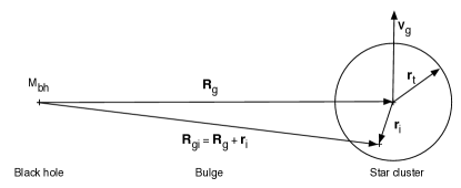
Figure 1: Sketch of the geometry of the problem as seen from the galactocentric reference frame. The vector $\mathbf{r}_{g}$ points from the Galactic centre to the star cluster centre. The vector $\mathbf{r}_{i}$ points from the star cluster centre to the position of the $i$th star. The orbital velocity of the star cluster has been denoted as $\mathbf{V}_{g}$.

The computer program nbody6gc which is used in this study is a variant of the $N$-body program nbody6++ (Aarseth 1999, 2003, Spurzem 1999) suited for massively parallel computers. The code nbody6++ is a variant of the direct $N$-body code nbody6 (Aarseth 1999, 2003) for single-processor machines. A fourth-order Hermite scheme, applied first by Makino & Aarseth (1992), is used for the direct integration of the $3N$ Newtonian equations of motion of the $N$-body system. It uses adaptive and individual time steps, which are organised in hierarchical block time steps, the Ahmad-Cohen neighbour scheme (Ahmad & Cohen 1973), Kustaanheimo-Stiefel (KS) regularisation of close encounters (Kustaanheimo & Stiefel 1965) and Chain regularisation (Mikkola & Aarseth 1990, 1993, 1996,1998).

2.1 Cluster orbit

We denote the radii, velocities and accelerations related to the Galactic centre with capital letters and those related to the star cluster with lower case letters. Figure 1 shows the geometry of the problem: A star cluster is orbiting around the Galactic centre. The potential in which the star cluster moves is the sum of the Kepler potential of a super-massive black hole and a scale free potential of the central region of the Galactic bulge (cf. Section 3.1). The two first-order equations of motion for the star cluster orbit read

$$\mathbf{V}_{g}(t) = \dot{\mathbf{R}}_{g},$$ (1)

$$\dot{\mathbf{V}}_{g}(t) = -\nabla\Phi_{g}(|\mathbf{R}_{g}|)+\mathbf{A}_{\rm df},$$ (2)

where $\mathbf{R}_{g},\mathbf{V}_{g},\Phi_{g}$ and $\mathbf{a}_{\rm df}$ are the position vector, velocity vector, gravitational potential of the Galactic centre region and deceleration due to dynamical friction and the dot denotes the derivative with respect to time. The equations of motion (1) and (2) for the star cluster orbit with respect to the Galactic centre are solved using an $8$th-order composition scheme (McLachlan 1995; for the idea see Yoshida 1990) with implicit midpoint method (e.g. Mikkola & Aarseth 2002), thereby including a realistic dynamical friction force. Although the symplectic composition schemes are by construction suited for Hamiltonian systems, they can be used for dissipative systems as well if the dissipative force is not too large. In our case, four iterations turned out to be sufficient to guarantee an excellent accuracy of the scheme.

We use a cluster membership criterion such that the dynamical friction force is based only on the total mass of the cluster members. We define a membership radius $r_{m}$ by the condition

$$\overline{\rho}_{cl}=\frac{3M_{cl}(r_{m})}{4\pi r_{m}^{3}}=\rho_{g}(R_{g})$$ (3)

as the radius where the mean density $\overline{\rho}_{cl}$ in the star cluster is equal to the local bulge density at the cluster centre which is located at radius $R_{g}$. This radius differs from the tidal radius (King 1962) only by a factor of order unity. Stars within twice the membership radius are defined as cluster members.

2.2 Stellar orbits

On the other hand, the equations of motion for the orbits of stars in the star cluster are solved by the standard nbody6/nbody6++ routines using the $4$th-order Hermite scheme (Makino & Aarseth 1992), KS or chain regularisation including the full 3D tidal forces from the super-massive black hole and the Galactic bulge. The tidal force is added as a perturbation to the KS regularisation. The following quantities are involved:

1. The specific force on the $i$th particle due to all other stars (cluster members and non-members) is given by

   $$\mathbf{a}_{i}=G\sum_{\begin{subarray}{c}j=1\\ j\not=i\end{subarray}}^{N}m_{j}\frac{\mathbf{r}_{ji}}{|\mathbf{r}_{ji}|^{3}},$$ (4)

   where $N$, $G$, $\mathbf{r}_{ji}=\mathbf{r}_{j}-\mathbf{r}_{i}$, $m_{j}$ are the particle number, the gravitational constant, the relative position vector between the $i$th and $j$th particles and the mass of the $j$th particle, respectively.

2. The specific force due to the Galactic centre at the position of the cluster centre is

   $$\mathbf{A}_{g}=-\left(\frac{GC}{R_{g}^{2-\alpha}}+\frac{GM_{bh}}{R_{g}^{2}}\right)\frac{\mathbf{R}_{g}}{R_{g}},$$ (5)

   where $C$, $M_{bh}$ and $\alpha$ are the normalisation of the scale free bulge mass profile (see Section 3.1), the mass of the super-massive black hole and the cumulative mass profile power law index.

3. The specific force exerted on particle $i$ due to the Galactic centre is given by

   $$\mathbf{A}_{gi}=-\left(\frac{GC}{R_{gi}^{2-\alpha}}+\frac{GM_{bh}}{R_{gi}^{2}}\right)\frac{\mathbf{R}_{gi}}{R_{gi}},$$ (6)

4. The deceleration due to dynamical friction is given by

   $$\mathbf{A}_{df}=-\frac{4\pi G^{2}\rho_{g}M_{cl}}{V_{g}^{2}}\ln\Lambda\,\chi(V_{g})\,\frac{\mathbf{V}_{g}}{V_{g}}$$ (7)

   where $\rho_{g}$, $M_{cl}$, $\mathbf{V}_{g}$ and $V_{g}$ are the local bulge density at the position of the star cluster centre, the star cluster mass and the velocity vector and modulus of the Galactic centre, respectively. Furthermore, $\ln\Lambda$ is the Coulomb logarithm which results from the integral over impact parameters and $\chi(v_{g})=\int_{0}^{V_{g}}f(v)d^{3}v$ is the result of the integration of the distribution function $f(v)$ of light particles over velocity space. For the Coulomb logarithm $\ln\Lambda$, we use according to Just & Peñarrubia (2005)

   $$\ln\Lambda = \ln\left(\frac{b_{1}}{b_{0}}\right),$$ (8)

   $$b_{1}^{2} = b_{0}^{2}+L^{2},\ \ \ \ \ b_{0}=r_{V},\ \ \ \ \ L=\frac{\rho_{g}}{\nabla\rho_{g}}$$ (9)

   where $b_{1}$, $b_{0}$, $L$ are the maximum and minimum impact parameters and the local scale length of the bulge density profile, respectively, and $r_{V}=GM_{cl}^{2}/(4|E_{cl}|)\approx r_{h}$ is the virial radius of the star cluster (where $E_{cl}$ is the internal energy of the star cluster and $r_{h}$ is the half-mass radius).

In the galactocentric reference frame, the total force on the $i$th particle would be given by

$$\mathbf{A}_{tot,i,gc} = \mathbf{a}_{i,gc}+\mathbf{A}_{gi,gc}+\mathbf{A}_{df,gc}\ \ \ \ \ \mathrm{memb.}$$ (10)

$$\mathbf{A}_{tot,i,gc} = \mathbf{a}_{i,gc}+\mathbf{A}_{gi,gc}\ \ \ \ \ \ \ \ \ \ \ \ \ \ \ \ \,\mathrm{non-memb.}$$ (11)

where the subscript “gc” denotes “galactocentric”. However, we choose the cluster rest frame as reference frame for our simulations. This is necessary, because Aarseth’s family of $N$-body programs is adapted to this reference frame and assumes that the cluster centre is close to the origin of coordinates. This guarantees a sufficient accuracy of the Hermite scheme which is used for the orbit integration. On the other hand, this choice of the reference frame implies that the Galactic centre is modelled as a pseudo-particle which orbits around the cluster centre. We keep in mind that a transformation from the galactocentric frame to the cluster rest frame implies that $\mathbf{r}_{i}$, $\mathbf{R}_{g}$, $\mathbf{V}_{g}$ and $\mathbf{R}_{gi}$ in (4) - (7) change their sign. This implies that

$$\mathbf{a}_{i,cl} = -\mathbf{a}_{i,gc},\ \ \ \ \ \mathbf{A}_{g,cl}=-\mathbf{A}_{g,gc},$$ (12)

$$\mathbf{A}_{gi,cl} = -\mathbf{A}_{gi,gc},\ \ \ \ \ \mathbf{A}_{df,cl}=-\mathbf{A}_{df,gc}$$ (13)

where the subscript “cl” denotes the cluster frame. It is then convenient for the force computations to transform to a reference frame in which the initial cluster centre is force-free. Since this frame is accelerated, an apparent force

$$\mathbf{A}_{app} = -\mathbf{A}_{g,cl}-\mathbf{A}_{df,cl}\ \ \ \ \ \mathrm{memb.}$$ (14)

$$\mathbf{A}_{app} = -\mathbf{A}_{g,cl}\ \ \ \ \ \ \ \ \ \ \ \ \ \ \ \ \mathrm{non-memb.}$$ (15)

appears. In the accelerated cluster frame the total force on the $i$th particle is therefore given by

$$\mathbf{A}_{tot,i,acl}=-\mathbf{A}_{tot,i,gc}+\mathbf{A}_{app}$$ (16)

where the subscript “acl” denotes the accelerated cluster frame. Thus the second-order equations of motion for the orbits of the cluster stars read

$$\mathbf{a}_{tot,i,acl} = \mathbf{a}_{i,cl}+\mathbf{A}_{gi,cl}-\mathbf{A}_{g,cl}\ \ \ \ \ \ \ \ \ \ \ \ \ \ \ \mathrm{memb.}$$ (17)

$$\mathbf{a}_{tot,i,acl} = \mathbf{a}_{i,cl}+\mathbf{A}_{gi,cl}-\mathbf{A}_{g,cl}-\mathbf{A}_{df,cl}\ \ \ \,\mathrm{n.-m.}$$ (18)

It can be seen that in the accelerated cluster frame an individual star experiences only the differential tidal force between its own location and the cluster centre.

We applied a density centre correction in certain intervals to correct for the displacement of the density centre. This was done in order to retain a consistent treatment of dynamical friction since the dynamical friction force is determined from the approximation that the star cluster mass is concentrated in the origin of coordinates.

2.3 Energy check

The specific energy $e_{i}$ of a particle is calculated in the galactocentric reference frame:

$$e_{i}=\frac{1}{2}(\mathbf{v}_{i}+\mathbf{V}_{g})^{2}+\Phi_{i,int}+\Phi_{i,ext}+\int_{t_{0}}^{t_{1}}\mathbf{a}_{df}\cdot\mathbf{V}_{gi}\,dt$$ (19)

where $\Phi_{i,int}=-G\sum_{j=1(\not=i)}^{N}m_{j}/{(|\mathbf{r}_{i}-\mathbf{r}_{j}}|)$ is the full internal potential of the $N$-body system, $\Phi_{i,ext}$ is the external potential of the Galactic centre and the last term is the energy loss due to dynamical friction. Using these terms, we calculate a total energy $E_{1}$. A factor $1/2$ has to be included in the summation of the potential energy of the $N$-body system. Note that the individual terms in (19) have quite different orders of magnitude. On the other hand, the orbital energy $E_{2}$ of the star cluster in the galactocentric reference frame is given by

$$E_{2} = \frac{1}{2}M_{cl}\mathbf{V}_{g}^{\,2}+M_{cl}\Phi_{ext}\left(|\mathbf{R}_{g}\right|)$$ (20)

$$+\int_{0}^{t}M_{cl}\,\mathbf{a}_{df}\cdot\mathbf{V}_{g}\,dt+\int_{0}^{t}\frac{\dot{M_{cl}}}{M_{cl}}E_{2}\,dt$$

where the last two terms on the right-hand side are corrections due to dynamical friction and tidal mass loss of the star cluster, respectively. Both energies $E_{1}$ and $E_{2}$ are checked at regular intervals for conservation. We note that the problem of a star cluster orbiting in a galactic tidal field has two energy scales related to the internal energy of the star cluster and the external energy of the tidal field. Tidal heating can transfer external energy from the larger scale into internal energy. The program nbody6gc conserves the energy within the cluster to a sufficient degree such that two-body relaxation is not suppressed (cf. Ernst 2009 for more details).

3 Theory

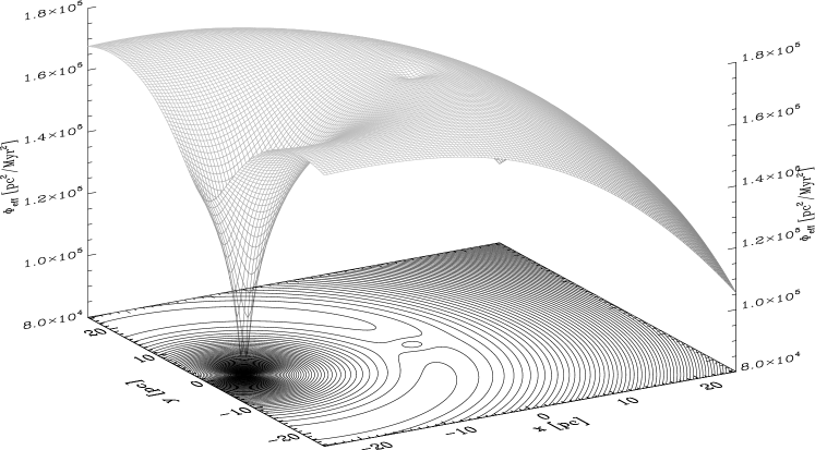
Figure 2: Effective potential for a star cluster in the centre of a galaxy ($z=0$ plane). The large potential well is due to the Galactic centre and the small one is due to the star cluster.

3.1 Galactic centre model

In the following Sections, we will use parameter values close to those of the centre of the Milky Way, since these parameters are better known than those of any other centre of a galaxy.

For the very central region of the Galactic bulge, we use a spherically symmetric scale free model (i.e. a model which is self-similar under scaling of lengths). The potential $\Phi$, cumulative mass $M$ and density $\rho$ are given by

$$\Phi(u) = \left\{\begin{array}[]{l}\Phi_{0}\,u^{\alpha-1}\ \ \ \ \ \alpha\not=1,\\ \Phi_{0}^{\prime}\,\ln u\ \ \ \ \ \ \alpha=1\end{array}\right.$$ (23)

$$M(u) = M_{0}\,u^{\alpha}$$ (24)

$$\rho(u) = \rho_{0}\,u^{\alpha-3}$$ (25)

where

$$u = R/R_{0},\ \ \ \ \ \rho_{0}=\frac{\alpha}{4\pi}\frac{M_{0}}{R_{0}^{3}},$$ (26)

$$\Phi_{0} = \frac{1}{\alpha-1}\frac{GM_{0}}{R_{0}}=\frac{4\pi G}{\alpha(\alpha-1)}\rho_{0}R_{0}^{2},$$ (27)

$\alpha$ is the power law exponent of the cumulative mass profile, $G$ is the gravitational constant and $R_{0}$ is a length unit (which is not inherent in nature but simply a human convention).

The circular frequency $\omega$ is given by

$$\omega(u)=\omega_{0}u^{(\alpha-3)/2},\ \ \ \ \ \omega_{0}=\sqrt{\frac{4\pi G\rho_{0}}{\alpha}}$$ (28)

The ratio of the epicyclic frequency $\kappa$ to the circular frequency $\omega$ is given by

$$\beta=\frac{\kappa}{\omega}=\sqrt{2\left[\frac{d\ln\omega}{d\ln u}+2\right]}=\sqrt{\alpha+1}$$ (29)

The angular momentum of the circular orbit is given by

$$L(u)=L_{0}u^{(\alpha+1)/2},\ \ \ \ \ L_{0}=\omega_{0}R_{0}^{2}.$$ (30)

Parameter	Value	Parameter	Value
$\alpha$	1.2	$E_{J}(L_{1})$ [pc2Myr-2]	1.67546e5
$R_{0}$ [pc]	20	$E_{J}(L_{2})$ [pc2Myr-2]	1.67592e5
$M_{0}$ [$M_{\odot}$]	1.67459e8	$E_{J}(L_{3})$ [pc2Myr-2]	1.65965e5
$\rho_{0}$ [$M_{\odot}$pc-3]	1998.90	$\Phi_{\rm eff,tid}(R_{0})$ [pc2Myr-2]	1.69502e5
$\Phi_{0}$ [pc2 Myr-2]	1.88335e5	$x(L_{1})$ [pc]	-2.66618
$\omega_{0}$ [Myr-1]	9.704	$x(L_{2})$ [pc]	2.78522
$M_{1}$ [$M_{\odot}$]	$10^{6}$
$r_{1}$ [pc]	$1.20213$	$G$ [pc3 $M_{\odot}^{-1}$ Myr-2]	$(222.3)^{-1}$

Table 1: Parameters used for the model of the Galactic centre region (Section 3.1) and the Plummer models (Section 3.2) which are used in Sections 3.3 and 3.4. $C(L_{i})$ and $x(L_{i})$ the value of the effective potential at the Lagrange point $L_{i}$ and its location, respectively and $G$ is the gravitational constant.

The parameters of our models are given in Table 1. The value of $M_{0}$ corresponds to $M_{0}(R_{0}=1\ \mathrm{pc})=4.6\times 10^{6}M_{\odot}$. The stellar mass within the central parsec is not easy to determine (see Schödel et al. 2007, Genzel et al. 2003 and also the review by Mezger, Duschl & Zylka 1996).

The simple numerical calculations in Sections 3.3 and 3.4 have been done without a black hole at the Galactic centre. Nevertheless, in our $N$-body calculations, we added the contribution of a super-massive black hole of mass $M_{\bullet}=3.6\times 10^{6}M_{\odot}$ (Eisenhauer et al. 2005). However, the influence radius (Frank & Rees 1976) of the Galactic super-massive black hole is only $1-2$ pc which is small compared to the galactocentric radii used in this study.

3.2 Star cluster model

For the star clusters, we use Plummer models for the simple numerical calculations in Sections 3.3 and 3.4 and King models (King 1966) for all $N$-body models in Section 4.

The Plummer model is given by

$$\Phi(v) = -\Phi_{1}\frac{1}{\sqrt{1+v^{2}}}$$ (31)

$$M(v) = M_{1}\frac{v^{3}}{\left[1+v^{2}\right]^{3/2}}$$ (32)

$$\rho(v) = \rho_{1}\frac{1}{\left[1+v^{2}\right]^{5/2}}$$ (33)

with the dimensionless radius $v=r/r_{1}\geq 0$ and the Plummer radius

$$r_{1}=\frac{GM_{1}}{\Phi_{1}}=\left(\frac{3M_{1}}{4\pi\rho_{1}}\right)^{1/3}$$ (34)

where $M_{1}$ is the total cluster mass, $-\Phi_{1}$ is the central potential and $\rho_{1}$ the central density, all of them being finite. The parameters of the Plummer models are given in Table 1. The parameters of the King models which we use for the $N$-body simulations are given in Table 2.

King models ($W_{0}=6$):
In general: $M_{\rm cl}=10^{6}M_{\odot},r_{h}=1.64\ {\rm pc},r_{t}=11.2\ {\rm pc}$;
K1 ($N=10^{3}$), K2 ($N=2\times 10^{3}$), K3 ($N=5\times 10^{3}$),
K4 ($N=10^{4}$), K5 ($N=2\times 10^{4}$), K6 ($N=3\times 10^{4}$),
K7 ($N=5\times 10^{4}$), K8 ($N=7\times 10^{4}$), K9 ($N=10^{5}$)

Table 2: Parameters of the $N$-body runs with King models. $W_{0},c$ and $r_{h}$ are the dimensionless central potential, the concentration and the half-mass radius of the King model, respectively, $N$ is the particle number and $M_{\rm cl}$ is the total cluster mass (which is only needed to calculate a dynamical friction force).

3.3 Effective potential

Figure 3: Zoom into the star cluster region of Figure 2.

Figure 4: Zoom into the star cluster region of Figure 2 along the $x$ axis with $y=0$. The Galactic centre lies in negative $x$ direction. It can be seen that the Lagrangian points $L_{1}$ and $L_{2}$ lie at different energies and at different distances from the cluster centre due to the asymmetry of the effective potential with respect to $x=0$. The dashed line marks the effective tidal potential. The solid line is the full potential with the added contribution of a Plummer potential.

In this and the following Section, we use the parameters given in Table 1. The length unit $R_{0}$ corresponds to the radius $R_{C}$ of the circular orbit, i.e. we have $R_{0}=R_{C}$.

Since we are considering a circular orbit, it is convenient to study the physics in a reference frame which is co-rotating with the frequency $\omega_{C}=\omega_{0}$ of the circular orbit. The star cluster centre is taken as the origin of coordinates. We choose a right-handed coordinate system where the $x$-axis points away from the Galactic centre and the $y$-axis points in the orbital direction of the star cluster orbit around the Galactic centre. In this reference frame, centrifugal and Coriolis forces naturally appear according to classical mechanics. The potential in which a particle moves is the superposition of the effective tidal potential and the star cluster potential. For short we will call this the effective potential.

The effective potential is shown in Figure 2. It is given by the expression

$$\Phi_{\rm eff}\left(x,y,z\right) = \Phi_{0}\left(\frac{\sqrt{(x+R_{0})^{2}+y^{2}+z^{2}}}{R_{0}}\right)^{\alpha-1}$$ (35)

$$- \frac{1}{2}\omega_{0}^{2}\left[\left(x+R_{0}\right)^{2}+y^{2}+z^{2}\right]$$

$$- \frac{GM_{1}}{\sqrt{R_{1}^{2}+x^{2}+y^{2}+z^{2}}}$$

Note that $\Phi_{0},\omega_{0}$ and $R_{0}$ are related by $\Phi_{0}=\omega_{0}^{2}R_{0}^{2}/(\alpha-1)$. In Equation (35), the first term is the gravitational potential of the central region of the Galactic bulge, the second term is the centrifugal potential and the last term is the Plummer potential of a star cluster. Note that the bulge potential is not well behaved in the limit $R_{0}\rightarrow 0$ if there is no black hole. However, the physics considered in this work happens close to the radii of the circular orbits. We note that the Jacobi energy per unit mass $E_{J}=\left(\dot{x}^{2}+\dot{y}^{2}+\dot{z}^{2}\right)/2+\Phi_{\rm eff}(x,y,z)$ is a conserved quantity in the co-rotating reference frame.

The tidal terms (i.e. the first two terms on the right-hand side) of Equation (35) can be expanded in a Taylor series around the star cluster centre $(x,y,z)=(0,0,0)$. Up to the $5$th order, the solution is given in Appendix A. The expansion up to the second order coincides with the tidal approximation which is a linear approximation of tidal forces. This approximation can be used to study the dynamics in star clusters on circular orbits which are far away from the Galactic centre. We stress, however, that we used the exact expressions for all computations in this study.

Figure 3 shows a zoom into the equipotential lines around the star cluster region of Figure 2. Figure 3 also shows the location of the Lagrange points $L_{1}$ and $L_{2}$. As usual, $L_{1}$ lies on the negative $x$-axis (between the cluster centre and the Galactic centre) while $L_{2}$ lies on the positive $x$-axis. $L_{1}$ and $L_{2}$ are saddle points of the effective potential. It can be seen that at the locations of $L_{1}$ and $L_{2}$, the surface in Figure 2 is curved differently along the $x-$ and $y-$axes.

Figure 4 shows the effective potential in the star cluster region along the line connecting the Galactic centre with the star cluster centre. The dashed line shows only the effective tidal potential $\Phi_{\rm eff,tid}$. The corresponding 1D Taylor series of $\Phi_{\rm eff,tid}$ along the $x$-axis around $x=0$ ($y=z=0$) is given by the power series

$$\Phi_{\rm eff,tid} \approx \frac{1}{2}\left(\frac{3-\alpha}{\alpha-1}\right)\omega_{0}^{2}R_{0}^{2}+\frac{1}{2}(\alpha-3)\omega_{0}^{2}x^{2}$$ (36)

$$+\sum_{k=3}^{\infty}\left\{\left[\prod_{l=2}^{k}(\alpha-l)\right]\frac{\omega_{0}^{2}}{R_{0}^{k-2}}\frac{x^{k}}{k!}\right\}$$

Higher-order terms lead to an asymmetry with respect to $x=0$ which becomes important in the vicinity of the Galactic centre. A non-linearity in the tidal forces is related to this asymmetry. Such non-linear effects can be seen in Poincaré surfaces of section. The solid line in Figure 4 shows the full effective potential. It is the superposition of the effective tidal potential and the star cluster potential. The Lagrange points $L_{1}$ and $L_{2}$ lie at slightly different energies and at slightly different distances from the star cluster centre whose position we denoted as as $L_{3}$. The energies and locations of the Lagrange points are given in Table 1.

We stress that this picture is only valid for a star cluster orbit which is exactly circular. The region above the tidal effective potential (dashed line in Figure 4) is energetically forbidden for the cluster orbit. As soon as it becomes eccentric, the cluster centre no longer remains at the position of the extremum of the effective tidal potential but oscillates around $x=0$ and is reflected either at the centrifugal or the gravitational barrier. This oscillation leads to oscillations of the Jacobi energies of the Lagrangian points $L_{1}$ and $L_{2}$ on the orbital time scale of the star cluster orbit and can change the dynamics dramatically.

3.4 Poincaré surfaces of section

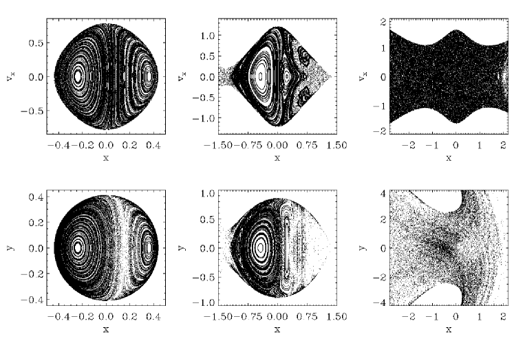
Figure 5: Poincaré surfaces of section. Left column: Deep in the potential well of the star cluster at $C=1.66638e5$ pc²/Myr². Middle column: At $E_{J}=E_{J}(L_{2})$. Right column: Above the Jacobi energies of $L_{1}$ and $L_{2}$ at $E_{J}=1.68845e5$ pc²/Myr².

Figure 5 shows a few Poincaré surfaces of section for the orbit with Parameters given in Table 1 which is exactly circular.

The left column of Figure 5 shows two Poincaré surfaces of section at a Jacobi energy deep in the potential well of the star cluster. The equipotential line corresponding to this Jacobi energy (which corresponds to the envelope of the lower surface of section in the left column of Figure 5) almost has a circular shape. The Poincaré surfaces of section at this Jacobi energy show that all orbits are regular and confined to invariant curves by a third integral. Such a third integral can usually be represented by a power series expansion where the lowest order is the angular momentum which would be exactly conserved if the system were spherical. Since the system is in fact not exactly spherical, the angular momentum slightly oscillates around some value (see e.g. Figure 3-5 in Binney & Tremaine 1987).

The middle column of Figure 5 shows two Poincaré surfaces of section at the Jacobi energy $E_{J}=E_{J}(L_{2})$ which corresponds to the Lagrange point $L_{2}$. The equipotential lines are open around $L_{1}$ and particles can escape towards the Galactic centre. The phase space is divided between regular and chaotic regions.

The right column of Figure 5 shows two Poincaré surfaces of section at a Jacobi energy which is higher than the value of the effective potential at both Lagrange points $L_{1}$ and $L_{2}$. The equipotential lines are wide open around $L_{1}$ and $L_{2}$ and particles can escape in both directions either into the leading or the trailing tidal arm. All orbits are chaotic.

4 Results

4.1 Tidal arm properties

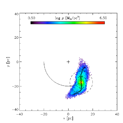
Figure 6: The model K9 at $t=0.22$ Myr. The Galactic centre is marked with a cross. The star cluster orbit is shown as a solid line. The dashed lines mark once and twice the membership radius. We look in the direction of the Galactic north pole. The short and long marks of the tidal arm coordinate system correspond to multiples of $1$ and $5$ pc, respectively.

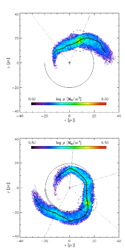
Figure 7: Further evolution of the model K9. Top panel: At $t=0.43$ Myr. Bottom panel: At $t=0.87$ Myr. The dotted lines from the Galactic centre show the angles between density maxima in the leading and trailing arm, respectively, with respect to the star cluster centre.

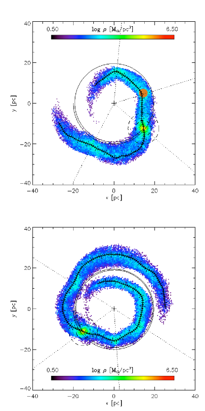
Figure 8: A standing density wave has developed in the model K9. Top panel: At $t=0.87$ Myr. A spherical cloud of tracer particles has been placed into the first clump (brown colored). Bottom panel: At $t=1.30$ Myr (without the tracer particles).

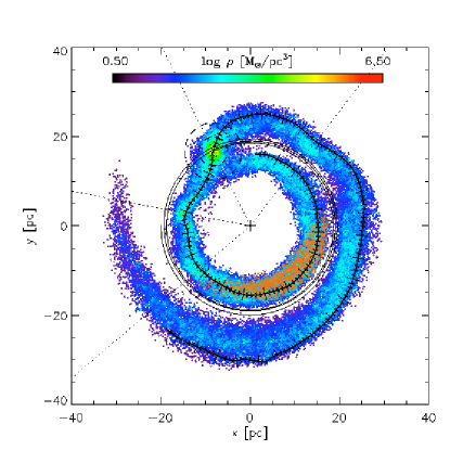
Figure 9: The model K9 at $t=1.74$ Myr. The tracer particles have travelled further while the wave maximum still persists. The leading and trailing arms have wound up. They are separated by the potential wall of the effective potential. The tip of the leading arm has hit the remnant of the star cluster again. We applied a weighting exponent to the particle mass in the expression (50).

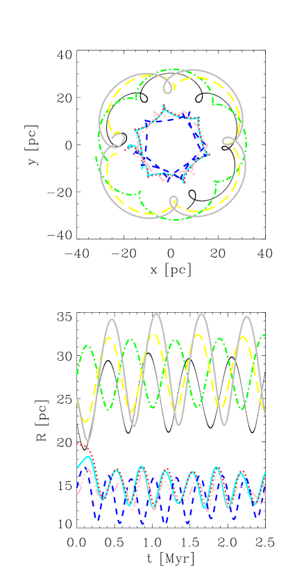
Figure 10: Top panel: Motion on cycloids within the tidal arms for a few particles in the model K9. The particles escape from locations near the cluster centre at (-20,0) either into the leading or the trailing arm. Bottom panel: Amplitude as a function of time for the same orbits. Small deviations from the harmonic motion can be seen which may be apparent deviations due to a slight change of the orbital frequency by dynamical friction or a deflection by 2-body encounters.

Figure 11: Histograms for the leading and trailing arms. All particles within twice (top panel) or once (middle panel) the initial tidal radius or outside of $25$ degrees around the density maximum in the first clump have been excluded from the statistics. We neglected deviations from the harmonic motion for the top and middle panel. Top panel: Epicentre radius distribution. Middle panel: Epicyclic period distribution. We set the bin frequency equal to the data output frequency of our code in order to avoid an unphysical higher harmonic in the histogram. Bottom panel: Distribution of dimensionless angular momentum differences.

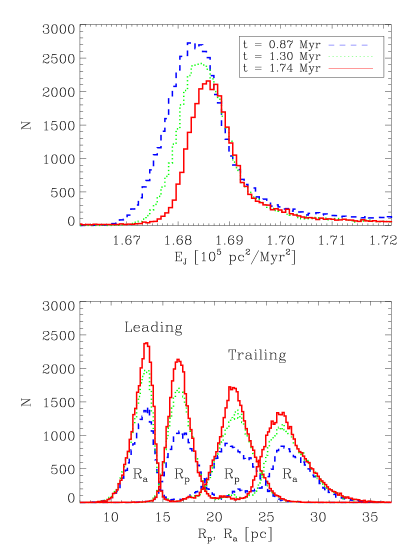
Figure 12: Top panel: Distribution of Jacobi energies. Bottom panel: Histogram of peri- and apocentre radii of the cycloid orbits in the tidal arms.

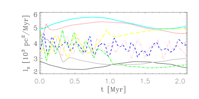
Figure 13: The $z$-component of angular momentum with respect to the Galactic centre for a few orbits. In the cluster the angular momentum is not conserved since the cluster potential breaks the axisymmetry of the effective potential. In the tidal arms the angular momentum is only approximately conserved.

Figures 6 - 9 show the formation of the tidal arms for model K9. The initial $90$% Lagrangian radius has been taken to be equal to the membership radius $r_{m}$ in Equation (3). The star cluster dissolves in a spiral-like structure. The leading tidal arm consists of particles which pass the inner Lagrange point $L_{1}$, while the trailing arm is formed by particles which pass the outer Lagrange point $L_{2}$. The galactocentric radius $R_{C}$ of the circular orbit is shown as a solid line. It decays very slowly due to dynamical friction with the Coulomb logarithm which was modified according to Equations (8) and (9). The initial value for the model K9 is $\ln\Lambda\approx 1.7$. Most particles of the leading arm have galactocentric radii less than $R_{C}$ while most particles of the trailing arm have radii larger than $R_{C}$. The dashed lines mark once and twice the membership radius $r_{m}$.

We have introduced a local coordinate system according to the description in Appendix B. We denote the coordinate along the tidal arms as $w$, where negative values refer to the leading arm and positive values to the trailing arm. The short and long marks correspond to multiples of $1$ and $5$ pc, respectively.

The color coding is according to the logarithm of the stellar density. The density clearly peaks in the cluster centre. However, one can observe clumps in the tidal arms where the density has local maxima. An indication for the presence of such clumps in tidal arms can already be found in the observations of Palomar 5 (Odenkirchen et al. 2001, 2003). The clumps have been first noticed in simulations by Capuzzo Dolcetta, di Matteo and Miocchi (2005) and were investigated further by di Matteo, Capuzzo Dolcetta & Miocchi (2005). They noted already the wave-like nature of this phenomenon.

The top panel of Figure 8 shows a spherical cloud of tracer particles (coloured brown). Figure 9 shows how the tracer particles have travelled further into the tidal arm while the position of the density maximum in the clump stayed (approximately) constant. Thus the clumps can be interpreted as wave knots of a density wave.

A theoretical explanation for such clumps was published in Küpper, Macleod & Heggie (2008). The top panel of Figure 10 shows for a few particles that they move on cycloids. The clumps appear at the position where many of the loops or turning points of the cycloids overlap. For a more detailed theory, see Just et al. (2009). The bottom panel of Figure 10 shows the radius as a function of time. We find approximate harmonic motion in the tidal arms.

The dotted lines from the Galactic centre in Figures 7, 8 and 9 show the angles $\varphi_{0}$ between density maxima in the leading and trailing arm. In order to plot these angles we determined the $w$ coordinate of the maxima in the mean density (cf. the top panel of Figure 15 below) and obtained the corresponding Cartesian coordinates from our data files.

Figure 11 shows the histogram of the epicentre radii $R_{E0}$ of the cycloid orbits, the epicyclic periods $T_{\kappa 0}$, and the dimensionless angular momentum differences $\Delta L/L_{C}=(L-L_{C})/L_{C}$ for different times, where $L_{C}$ is the angular momentum of the circular orbit. For the epicentre radii (and the epicyclic periods), stars within twice (and once) the membership radius were not included in the statistics. The epicentre radii are given by the arithmetic mean of the last maximum and minimum in the epicyclic amplitude. The epicyclic period is given by the time between the last two minima in the epicyclic amplitude. Note that at $t=0.87$ Myr not all particles have completed one epicyclic period. For the dimensionless angular momentum differences we included only stars within 25 degrees around the density maximum in the clump. Thus one can see two side lobes in all panels corresponding to the leading and trailing arms. Figure 12 shows the distribution of Jacobi energies $E_{J,i}$ and the histogram of peri- and apocentre radii of the cycloid orbits in the tidal arms.

The angle $\varphi_{0}$ can be expressed as

$$\varphi_{L} = \frac{2\pi}{\beta}\left[1-\frac{\omega_{C}}{\omega}\right]$$ (37)

$$= \frac{2\pi}{\sqrt{\alpha+1}}\left[1-\left(1+\frac{\Delta L}{L_{C}}\right)^{\frac{3-\alpha}{\alpha+1}}\right]$$ (38)

where $\omega_{C}$ and $\omega$ are the circular frequencies at the radius $R_{C}$ of the circular orbit and in the vicinity of $R_{C}$, $\beta$ is given by Equation (29) and $\Delta L/L_{C}$ is the most frequent dimensionless angular momentum difference.

The subscript “L” refers in the following discussion to quantities which are expressed as a function of $\Delta L/L_{C}$, while the subscript “0” refers to quantities which are directly measured from the simulation.

The epicentre radius of the cycloids is given by

$$R_{EL}=R_{C}\left(1+\frac{\Delta L}{L_{C}}\right)^{\frac{2}{\alpha+1}}.$$ (39)

According to Just et al. (2009), the epicyclic amplitude can be expressed as

$$\Delta r_{L}=\sqrt{\frac{2}{\alpha+1}\left[\frac{3-\alpha}{2\alpha+2}R_{C}^{2}\frac{\Delta L^{2}}{L_{C}^{2}}+\frac{\Delta E_{J}}{\omega_{C}^{2}}\right]}$$ (40)

to second order in the dimensionless angular momentum difference, where $\Delta E_{J}=E_{J}-\Phi_{\rm eff,tid}(R_{C})$ is the Jacobi energy difference with respect to the effective tidal potential at $R_{C}$.

Table 3 shows a comparison of the measured angles, epicentre radii, epicyclic amplitudes, peri- and apocentres and the theoretical estimates from the dimensionless angular momentum difference. We give the measured angle $\varphi_{0}$, the estimate $\varphi_{L}$ according to Equation (38), the error $\Delta\varphi/\varphi_{0}=(\varphi_{0}-\varphi_{L})/\varphi_{0}$ in percent, the most frequent epicentre radius $R_{E0}$ in Figure 11, the epicentre radius $R_{EL}$ according to Equation (39), the most frequent epicyclic period $T_{\kappa 0}$ in Figure 11 and the theoretical epicyclic period $T_{\kappa}(R_{EL})$ using Equation (28) with the epicentre radius $R_{EL}$. Furthermore, we give the tidal radius $r_{t}=\left\{GM_{cl}/\left[(4-\beta^{2})\omega_{C}^{2}\right]\right\}^{1/3}$ (King 1962), the arc length $y_{0}=R_{C}\varphi_{0}$, the A factors (Just et al. 2009),

$$A_{y0}=\frac{1}{\pi}\frac{\sqrt{\alpha+1}}{3-\alpha}\frac{y_{0}}{r_{t}},\ \ \ \ \ A_{L}=\frac{|R_{E,L}-R_{C}|}{r_{t}}$$ (41)

where $A_{y0}$ is a first-order approximation and the error $\Delta A/A_{y0}=(A_{y0}-A_{L})/A_{y0}$ is in percent. We also give the most frequent peri- and apocentre radii $R_{P0}$ and $R_{A0}$ from Figure 12, the most frequent scaled Jacobi energy difference $\Delta E_{J}/\omega_{E}^{2}$ from Figure 12, the epicyclic amplitude $\Delta r_{L}$ from Equation (40) and the obtained peri- and apocentre radii $R_{PL}$ and $R_{AL}$, where $|R_{PL}-R_{EL}|=|R_{AL}-R_{EL}|=\Delta r_{L}$.

There are systematic errors in both $\Phi_{L}$ and $A_{L}$ and also in $R_{PL}$ and $R_{AL}$. The reason is shown in Figure 13. In the tidal arms the angular momentum is only approximately conserved. The reason is the influence of the cluster potential which breaks the axisymmetry of the effective potential. However, in the cluster the angular momentum changes in a much shorter time scale. An estimate for the cumulative perturbation $\Delta L$ of $L$ is given by

$$\Delta L=\Big{|}\int(\mathbf{R}\times\mathbf{a})\,dt\Big{|}\approx\frac{R\,\Phi_{\rm cl}}{V_{\rm drift}}.$$ (42)

where $\mathbf{a}$, $R=|\mathbf{R}|$, $\Phi_{\rm cl}$ and $V_{\rm drift}$ are the acceleration, galactocentric radius, potential energy of the cluster and the drift velocity, respectively. Thus a slow drift velocity increases the change in $L$. Here a more detailed theory is desirable.

#	$t$ [Myr]	Arm	Clump	$\Delta L/L_{C}$	$|\varphi_{0}|$ [deg.]	$|\varphi_{L}|$ [deg.]	$\Delta\varphi/\varphi_{0}$ [%]	$R_{C}(t)$ [pc]
1	0.87	lead.	1	-0.232	57.5	47.1	18.1	19.0
2	”	lead.	2	-0.273	67.6	55.7	17.6	”
3	”	trail.	1	0.320	68.6	61.9	9.8	”
4	1.30	lead.	1	-0.215	57.5	43.6	24.2	18.8
5	”	lead.	2	-0.227	53.3	46.1	13.5	”
6	”	trail.	1	0.276	68.4	53.6	21.6	”
7	1.74	lead.	1	-0.209	52.6	42.4	19.4	18.6
8	”	lead.	2	-0.205	51.5	41.5	19.4	”
9	”	trail.	1	0.273	64.2	53.0	17.4	”
#	$R_{E0}$ [pc]	$R_{EL}$ [pc]	$T_{\kappa 0}$ [Myr]	$T_{\kappa}(R_{EL})$ [Myr]	$r_{t}(t-T_{\kappa 0})$ [pc]	$y_{0}$ [pc]	$A_{y_{0}}$	$A_{L}$
1	14.9	14.9	0.32	0.35	2.67	19.1	1.88	1.54
2	”	14.2	”	0.34	”	22.4	2.20	1.80
3	24.2	24.5	0.55	0.55	2.87	22.7	2.07	1.92
4	14.7	15.1	0.33	0.36	2.40	18.9	2.07	1.54
5	”	14.9	”	0.35	”	17.5	1.91	1.63
6	24.7	23.5	0.51	0.53	2.63	22.4	2.23	1.79
7	14.7	15.0	0.32	0.36	2.21	17.1	2.03	1.63
8	”	15.1	”	0.36	”	16.7	1.98	1.58
9	24.0	23.2	0.51	0.53	2.29	20.8	2.38	2.01
#	$A_{R_{E0}}$	$\Delta A/A_{y0}$ [%]	$R_{P0}$ [pc]	$R_{A0}$ [pc]	$\Delta E_{J}/\omega_{E}^{2}$ [pc2]	$\Delta r_{L}$ [pc]	$R_{PL}$ [pc]	$R_{AL}$ [pc]
1	1.54	18.1	16.6	13.6	3.80	2.8	17.7	12.1
2	”	18.1	”	”	3.46	2.9	17.1	11.3
3	1.81	7.2	21.3	26.2	9.25	5.3	19.2	29.8
4	1.71	25.6	16.5	13.3	6.50	3.1	18.2	12.0
5	”	14.7	”	”	6.39	3.1	18.0	11.8
6	2.24	19.7	22.1	26.2	14.4	5.1	18.4	28.6
7	1.76	19.7	16.5	13.3	11.5	3.7	18.7	11.3
8	”	20.2	”	”	11.6	3.7	18.8	11.4
9	2.36	15.5	21.4	26.0	25.2	6.0	17.2	29.2

Table 3: Comparison of measurement and theory for the angles of the density maxima and the A factors. For explanations see the text.

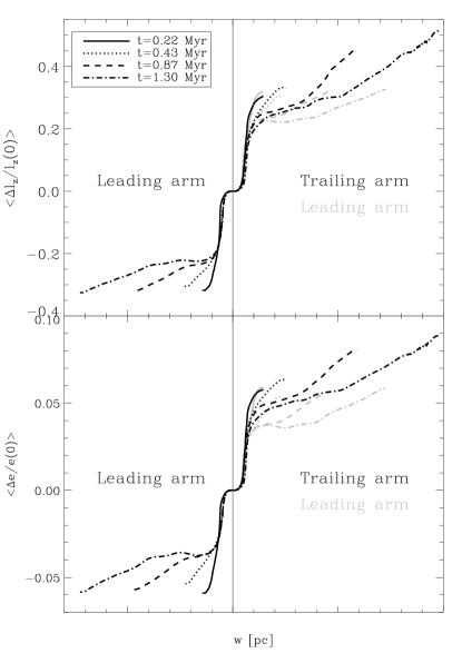
Figure 14: Top panel: Time evolution of the angular momentum difference between the cluster center and the position in the tidal arm for the model K9. The angular momentum difference is normalized by the angular momentum of the cluster center. In order to show the asymmetry between the leading and trailing arms, the lines for the leading arm have been rotated by 180 degrees about the origin and replotted in grey. Bottom panel: As in the top panel, but for the energy (internal and external) difference between the cluster center and the position in the tidal arm for the model K9. The energy difference is normalized by the energy of the cluster center.

Figure 15: Top panel: Time evolution of the mean density of stars along the tidal arms for the model K9. One can see that several density wave maxima develop with time. Bottom panel: Time evolution of the 1D velocity dispersion along the tidal arms for the model K9. The characteristic features in the mean density (top panel) can also be seen in the velocity dispersion.

Figure 16: Time evolution of the mean star cluster potential along the tidal arms for the model K9. One can see that the potential well is deeper in the beginning but gets shallower as the cluster loses mass.

For Figures 14 - 16, we averaged over spheres with a radius which was approximately equal to the width of the tidal arms in the $xy$ plane (see Appendix B for the details). Since the Figures were still noisy, we have used a median smoothing in addition. The width of the smoothing kernel has been taken to be twice the membership radius $r_{m}$ defined in Equation (3).

For four different times, the top panel of Figure 14 shows the $z$-component of the dimensionless mean angular momentum difference $\left[l_{z}(w)-l_{z}(0)\right]/l_{z}(0)$ along the tidal arms. The specific angular momentum was calculated with respect to the Galactic center. In order to show the asymmetry between the leading and trailing arms, the lines for the leading arm have been rotated by 180 degrees about the origin and replotted in grey. This kind of asymmetries arise from the geometry of the effective potential.

The bottom panel of Figure 14 shows the same for the mean energy difference $\left[e(w)-e(0)\right]/e(0)$. The specific energy was calculated with respect to the Galactic center. For the definition of the energy, see Section 2.3. A positive energy difference corresponds to the trailing arm while a negative energy difference corresponds to the leading arm. This is in accordance with the positive normalization in Equation (27) for the scale free potential in Equation (23). This Figure also shows an asymmetry between leading and trailing arm. What can be seen in this plot is that with the time more and more particles with a low energy difference with respect to the cluster center stream into the tidal arms. Thus the modulus of the mean energy difference falls off with time. In this connection it is worthwhile to mention that the particles with a low Jacobi energy stream into the tips of the tidal arms. This can be seen in Figure 9: The stars in the tips of the tidal arms are far away from the potential wall of the effective tidal potential which lies below the solid line of the orbit of the star cluster center.

The top panel of Figure 15 shows the density profile along the tidal arm coordinate $w$. At $t=0.43$ Myr, one clump can be seen in the leading arm. At $t=0.87$ Myr, two clumps can be seen in the leading arm and one in the trailing arm. At $t=1.30$ Myr, three clumps can be seen in the leading arm and two in the trailing arm.

The bottom panel of Figure 15 shows the profile of the 1D velocity dispersion along the tidal arm coordinate $w$. The averaging for the calculation of the velocity dispersion has been done in small spheres around the tidal arm coordinate system whose radius was approximately 1/5 of the width of the tidal arms in the $xy$ plane (see Appendix B for more details). The velocity dispersion profile also exhibits local maxima at the positions of the density maxima. This is in accordance with the notion that the clumps in the tidal arms occur at the positions where many of the loops or turning points of the cycloid orbits overlap. At these positions, the random velocities should exhibit maxima as well. Note that the first maximum in the leading arm at $t=0.43$ Myr cannot yet be seen clearly in the bottom panel of Figure 15. Figure 7 shows that this density maximum is still in the process of building up.

Figure 16 shows the profile of the cluster gravitational potential along the tidal arm coordinate $w$ at four different times. One can see that the potential well of the star cluster is deeper in the beginning but gets shallower as the cluster loses mass.

Figure 17: Evolution of the cluster mass within the tidal radius and the mass in the tidal arms for the model K9. It can be seen that more particles escape into the trailing arm than into the leading arm. The ratio of leading arm mass to trailing arm mass is always roughly 85%. The thin vertical dotted lines correspond to $t=0.22,0.43,0.87,1.30$ and $1.74$ Myr.

Figure 17 shows the evolution of the cluster mass contained within the tidal radius for the model K9. In addition, the mass in the tidal arms is shown as a function of time. It can be seen that more particles escape into the trailing arm than into the leading arm. In the relaxation-driven dissolution scenario this would be paradoxical since the inner Lagrange point $L_{1}$ is at a lower energy than the outer Lagrange point $L_{2}$ according to Figure 4. However, most stars are in the high-energy region of the star cluster. For these particles the phase space for escape into the trailing arm is larger than that for escape into the leading arm.

4.2 Lifetime scaling and RE classification

Figure 18: Scaling of the ratio of half-mass time $t_{half}$ to crossing time $t_{cr}$ as a function of the particle number $N$ for the models K1 - K9. The errors correspond to $1$ crossing time $t_{cr}$. We have $t_{cr}=0.123$ Myr in all models. The “third-” and “fifth-mass” times are also shown.

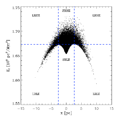
Figure 19: Projection of initial Jacobi energies of stars onto the $x-\Phi_{\rm eff}$ plane of Figure 4 for the model K9. The dashed lines mark the different regions of the Radius-Energy (RE) classification.

Figure 18 shows the scaling of the half-mass time as a function of the particle number. The half-mass time is the time after which the star cluster has lost half of its initial mass due to escaping stars. It also shows as dots the times, when the cluster has one third or one fifth, respectively, of its initial mass. The particle number in Figure 18 ranges from $N=10^{3}$ up to $N=10^{5}$. The $\chi^{2}$ fit of a power law shows that the half-mass time depends only slightly on the particle number $N$.

This is in contrast to the relaxation-driven dissolution of star clusters. If the dissolution is relaxation-driven, the stars are scattered above the escape energy (or the critical Jacobi energy) by two-body relaxation before they can escape through exits in the equipotential surfaces around the Lagrangian points $L_{1}$ and $L_{2}$. In this case the half-mass or dissolution time should depend more strongly on the particle number than in Figure 18. Baumgardt (2001) developed a detailed theory for the relaxation-driven dissolution of star clusters on circular orbits in a steady tidal field with back-scattering of potential escapers in which the half-mass time scales as $t_{half}\propto t_{rh}^{3/4}$.

Fukushige & Heggie (2000) give a hint for the understanding of the scaling of the half-mass time in our models. In Figure 19 one can see that the cluster fills the energetic region above the total effective potential of Figure 4. Many stars are initially outside of the tidal radius $\overline{r}_{L}=\left[x(L_{1})+x(L_{2})\right]/2$ and most particles have Jacobi energies $E_{J}$ per unit mass which are higher than the mean effective potential $\overline{E}_{J,L}=\left[E_{J}(L_{1})+E_{J}(L_{2})\right]/2$ of both Lagrange points $L_{1}$ and $L_{2}$. We initially have for the model K9 the following ratio of particle numbers:

$$\frac{N_{\rm r>\overline{r}_{L}}}{N_{\rm r<\overline{r}_{L}}}\approx 0.37\ \ \ \mathrm{and}\ \ \ \frac{N_{\rm E_{J}>\overline{E}_{J,L}}}{N_{\rm E_{J}<\overline{E}_{J,L}}}\approx 1.80.$$ (43)

The stars which are outside of $\overline{r}_{L}$ and the high-energy particles with respect to the critical Jacobi energy $\overline{E}_{J,L}$ can leave the cluster relatively fast as compared with the relaxation time, provided they are not bound by a non-classical integral of motion which would hinder their escape. Figure 5 shows that above a certain Jacobi energy threshold in the high-energy regions all orbits are chaotic and not subject to a non-classical integral of motion.

It is possible to classify the particles initially according to their membership to one of four regions:

1. Large Radius High Energy (LRHE) region

2. Small Radius High Energy (SRHE) region

3. Large Radius Low Energy (LRLE) region

4. Small Radius Low Energy (SRLE) region

The distinction between these regions is shown with dashed lines in Figure 19. We call this the Radius-Energy (RE) classification. The classification arises due to the existence of the Lagrange points $L_{1}$ and $L_{2}$ at proximate (or equal) Jacobi energies. For the model K9 with $N=10^{5}$, we initially have the following occupation numbers of the four regions,

$$N_{\rm LRHE}=24370,\ \ \ N_{\rm SRHE}=39854,$$

$$N_{\rm LRLE}=2831,\ \ \ N_{\rm SRLE}=32945.$$ (44)

In an exact treatment the critical equipotential line should be taken as the dividing line between small and large radii in the RE classification. However, in real $N$-body simulations it is more convenient to adopt the tidal radius for this purpose as has been done in the counting for Equations (44). Particles in the LRLE region are immediately lost due to the energy barrier if they are not bound to the cluster by a non-classical integral of motion. Particles in the LRHE and SRHE regions can mix dependent on their individual position and velocity. Particles in the SRLE region are bound to the cluster until they are lifted to the SRHE region by secular evolution or 2-body relaxation.

Particularly the ratio

$$\alpha_{M}=\frac{M_{\rm LRLE}+M_{\rm LRHE}+M_{\rm SRHE}}{M_{\rm SRLE}}$$ (45)

determines the physics of the dissolution process, where $M_{\rm LRLE}$, $M_{\rm LRHE}$, $M_{\rm SRHE}$ and $M_{\rm SRLE}$ are the occupation masses of the four regions. If $\alpha_{M}$ is close to zero the main process which leads to the dissolution of the cluster is two-body relaxation, which scatters stars from the SRLE region into the two high-energy regions. The larger the particle number $N$ is, the slower is this process. We speculate that $\alpha_{M}$ was very small for the old globular clusters in the halo of the Milky Way and that their dissolution is relaxation-driven, but that many young star clusters (open clusters or associations) with larger values of $\alpha_{M}$ may form at all times in the Milky Way and dissolve fast as compared with the Hubble time. If $\alpha_{M}$ is sufficiently large, mass loss from the SRLE region seems to be dominated by a self-regulating process of increasing Jacobi energy due to the weakening of the potential well of the star cluster, which is induced by the mass loss itself (Just et al. 2009). A simple estimation shows that the critical Jacobi energy $\overline{E}_{J,L}$ increases more slowly with time as compared with the Jacobi energy $E_{J}$ of a star in the non-stationary gravitational potential of the star cluster. While the particles in the LRLE, LRHE and SRHE regions of the star cluster move away from the cluster along the tidal arms, particles are continually shifted from the SRLE region into the two high-energy regions as the potential well of the star cluster gets shallower (cf. Figure 16). In addition, a fraction of particles is scattered from the SRLE region into the high-energy regions by two-body relaxation. The two-body relaxation leads to the small slope $0.127\pm 0.030$ in Figure 18. It is small since $\alpha_{M}$ is very large for the models K1 - K9. From the values in Equation (44) we obtain $\alpha_{M}\approx 2$ for the model K9 with the valid assumption that the particles of different mass are initially uniformly mixed in radius and Jacobi energy per unit mass.

If the physical tidal radius is equal to the radius where the density of the star cluster (King) model vanishes, we have $N_{\rm LRLE}=N_{\rm LRHE}=0$ and only two of the four regions are occupied with particles. This is the standard case used in $N$-body simulations of star clusters in a tidal field so far (e.g. Baumgardt & Makino 2003, Trenti, Heggie & Hut 2007, Ernst et al. 2007). In this case, $\alpha_{M}$ is small (typically a few percent) and the dissolution times are considerably $N$-dependent as we checked with a few models ($N=10^{3},2\times 10^{3},5\times 10^{3},10^{4},3\times 10^{4}$) using nbody6gc. Furthermore, in this case our preliminary models suggest that the dissolution time directly scales with a power of the relaxation time. However, a more detailed study seems to be essential. On the other hand, Tanikawa & Fukushige (2005) adopted initial models where the King cutoff radius was smaller or larger than the physical tidal radius. By decreasing the size of the initial star cluster further $\alpha_{M}$ can be forced to vanish.

We argue that the situation that the cluster is divided into the four regions of the RE classification (with certain occupation numbers and masses) is the typical situation for newly formed star clusters. A first crucial question is whether stars can form in all regions. The answer is yes, if the condition for star formation is fulfilled. According to the modern picture of gravo-turbulent star formation (e.g. Mac Low & Klessen 2004, Ballesteros-Paredes et al. 2007), supersonic turbulence and shocks create initial density enhancements in a molecular cloud. The formed molecular cloud core contracts gravitationally and fragments eventually. Finally, protostellar seeds form, accrete in-falling material and become main sequence stars. The condition for star formation is independent of the distinction between high- and low-energy regions of the effective potential. Thus one would expect that stars form initially in the high-energy regions and the SRLE region slowly builds up as more material moves towards the center of the new star cluster. Due to the turbulent structure within the molecular cloud it is also possible that a small fraction of stars forms in the LRLE region.

In the Galactic center, the supersonic shock and turbulent velocities must be high enough to form mean densities which withstand the tidal shear forces. According to Morris (1993), the critical mean number density for gravitationally bound clouds in the Galactic center region is given by

$$n_{crit}=10^{7}\ \mathrm{cm}^{-3}\left(\frac{1.6\ \mathrm{pc}}{R_{g}}\right)^{1.8},$$ (46)

where $R_{g}$ is the galactocentric radius.

The picture sketched above would be similar if the star cluster formation in the Galactic center is triggered by the collision of two clouds. For typical parameters (e.g. for the formation of clusters like Arches and Quintuplet) the rate of such cloud collisions in the Galactic center is low as compared with the reciprocal of the lifetime of OB stars and can be crudely estimated to be

$$\nu_{col} = 5\times 10^{-8}\ \mathrm{yr}^{-1}\left(\frac{M_{cloud}}{10^{6}\ M_{\odot}}\right)^{-1}$$ (47)

$$\times\left(\frac{N_{H_{2}}}{10^{23}\ \mathrm{cm}^{-2}}\right)^{-1}\left(\frac{\sigma_{v}}{20\ \mathrm{km\ s}^{-1}}\right)$$

where $M_{cloud}$, $N_{H_{2}}$ and $\sigma_{v}$ are the mass, the column density and the velocity dispersion of a cloud (Hasegawa et al. 1994, Stolte et al. 2008).

Finally, we note that the Jeans time scale is of the same order as the dissolution times of our models in the Galactic center. According to Hartmann (2002), who explored an earlier idea by Larson (1985), the Jeans (or fragmentation) time scale of a gaseous filament can be written as

$$\tau\approx 3.7\ \left(\frac{T}{10\ \mathrm{K}}\right)^{1/2}A_{V}^{-1}\ \mathrm{Myr}$$ (48)

where $T$ is the temperature and $A_{V}\approx 5$ is the visual extinction through the center of the filament (see also Klessen et al. 2004).

5 Discussion

We have studied the dissolution of star clusters in an analytic background potential of the Galactic centre by means of direct $N$-body simulations. We described in detail the algorithm of our parallel $N$-body program nbody6gc which is based on Aarseth’s series of $N$-body codes (Aarseth 1999, 2003, Spurzem 1999). It includes a realistic dynamical friction force with a variable Coulomb logarithm based on the paper by Just & Peñarrubia (2005). The initial value for the circular orbit of the model K9 is $\ln\Lambda\approx 1.7$. It turns out that, even for a $10^{6}\ M_{\odot}$ cluster, the dynamical friction force is too weak to let a cluster on a circular orbit at $R_{C}=20$ pc spiral into the Galactic centre within the lifetime of its most massive stars. Thus we did not resolve the “paradox of youth” (Ghez et al. 2003).

However, we have studied in detail the dynamics of dissolving star clusters on circular orbits in the Galactic centre. The key to the understanding of this dynamical problem is the gravitational potential which is the sum of the effective tidal potential and the star cluster potential. Along the orbit of the star cluster, the effective tidal potential resembles a parabolic wall. However, in the close vicinity of the Galactic centre there are deviations from the parabolic shape due to higher-order terms in the Taylor expansion of the effective tidal potential. Due to this asymmetry, the Lagrange points $L_{1}$ and $L_{2}$ lie at different energies.

We have studied in detail the properties of the tidal arms of a dissolving star cluster in a galactic centre. The density wave phenomenon found by Capuzzo Dolzetta, di Matteo & Miocchi (2005) and di Matteo, Capuzzo Dolcetta & Miocchi (2005) appears in our model K9. The angles of the clumps can be calculated with the theory from Just et al. (2009).

We have presented a method to study the structure of tidal arms by using an eigensolver. The eigensolver calculates numerically a 1D coordinate system along the tidal arms and calculates characteristic dynamical quantities along this coordinate system.

It may be of interest to note that more particles escape into the trailing tidal arm than into the leading tidal arm. For the high-energy particles the phase space for escape into the trailing arm is larger than that for escape into the leading arm. The fractions of initial conditions in the phase space for escape into the leading and trailing arm, respectively, have to be calculated numerically for several Jacobi energies. The result would be called the ‘basins of escape’ of the star cluster (e.g. Aguirre et al. 2001, Contopoulos 2002, Ernst et al. 2008). This kind of asymmetry between the arms does not depend on the particle number.

The half-mass times of our models K1 - K9 depend only weakly on the particle number which indicates that two-body relaxation is not the dominant mechanism leading to the dissolution. The reason is that the initial models are divided into four different regions in radius and specific Jacobi energy space. This division has been termed the Radius-Energy (RE) classification. The division of a newly formed star cluster into the four regions of the RE classification is probably a typical situation which is consistent with the modern picture of gravoturbulent star formation (e.g. Mac Low & Klessen 2004, Ballesteros-Paredes et al. 2007). If the ratio $\alpha_{M}$ (which has been defined in Section 4.2) is large enough, the dissolution is no longer relaxation-driven but the mass loss from the SRLE region is governed by a self-regulating process of increasing Jacobi energy due to the weakening of the potential well of the star cluster, which is induced by the mass loss itself (Just et al. 2009). Predictions about the fractions of stars which belong to the four different regions (i.e., the occupation numbers and masses) may be an important result of the emerging theory of star cluster formation. What are typical ratios of occupation numbers and masses in regions with efficient star formation? How do the occupation numbers, masses and their ratios differ between open and globular clusters? From the side of stellar dynamics the scaling problem of the dissolution times (Baumgardt 2001) needs to be solved for the new dissolution mechanism due to a non-stationary gravitational potential combined with the effect of two-body relaxation. In this paper, we also conjecture that the ratio $\alpha_{M}$ can be used to draw a distinction between associations, open and globular clusters, i.e. that the old globular clusters obey $\alpha_{M}\ll 1$ and that their dissolution is relaxation-driven, while the open clusters and associations obey $\alpha_{M}\gg 0$.

6 Acknowledgements

We thank Prof. Ortwin Gerhard and Dr. Kap-Soo Oh for many discussions related to an earlier version of the program nbody6gc and Dr. Godehard Sutmann for making us aware of the composition schemes. Also, we thank Prof. Douglas Heggie and an anonymous referee for two comments which, together with a plot of Dr. Peter Berczik, finally led to the RE classification.

AE gratefully acknowledges support by the International Max Planck Research School (IMPRS) for Astronomy and Cosmic Physics at the University of Heidelberg.

We thank the DEISA Consortium (www.deisa.eu), co-funded through EU FP6 projects RI-508830 and RI-031513, for support within the DEISA Extreme Computing Initiative.

Appendix A Taylor expansion of the effective tidal potential

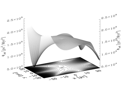
Figure 20: Taylor expansion of the effective tidal potential for the scale free model up to the $5$th order.

Usually a Cartesian Taylor expansion of the effective tidal potential is used. Up to $5$th order, the 3D Cartesian Taylor expansion of the effective tidal potential for the scale free model is given by

$$\Phi_{\rm eff,tid} \approx \frac{1}{2}\left(\frac{3-\alpha}{\alpha-1}\right)\omega_{0}^{2}R_{0}^{2}+\frac{1}{2}(\alpha-3)\omega_{0}^{2}x^{2}$$ (49)

$$+ (\alpha-3)(\alpha-2)\frac{\omega_{0}^{2}}{6R_{0}}x^{3}$$

$$+ (\alpha-3)\frac{\omega_{0}^{2}}{2R_{0}}x(y^{2}+z^{2})$$

$$+ (\alpha-4)(\alpha-3)(\alpha-2)\frac{\omega_{0}^{2}}{24R_{0}^{2}}x^{4}$$

$$+ (\alpha-4)(\alpha-3)\frac{\omega_{0}^{2}}{4R_{0}^{2}}x^{2}(y^{2}+z^{2})$$

$$+ (\alpha-3)\frac{\omega_{0}^{2}}{4R_{0}^{2}}y^{2}z^{2}$$

$$+ (\alpha-5)(\alpha-4)(\alpha-3)(\alpha-2)\frac{\omega_{0}^{2}}{120R_{0}^{3}}x^{5}$$

$$+ (\alpha-5)(\alpha-4)(\alpha-3)\frac{\omega_{0}^{2}}{12R_{0}^{3}}x^{3}(y^{2}+z^{2})$$

$$+ (\alpha-5)(\alpha-3)\frac{\omega_{0}^{2}}{8R_{0}^{3}}x(y^{4}+z^{4})$$

$$+ (\alpha-5)(\alpha-3)\frac{\omega_{0}^{2}}{4R_{0}^{3}}xy^{2}z^{2}$$

where $R_{0}$ and $\omega_{0}$ are the radius and the frequency of the circular orbit. This solution is shown in Figure 20 (which may be compared with Figure 2). It can be seen that this Taylor expansion cannot be used to study the properties of tidal arms in the Galactic centre. For extended tidal tails cylindrical coordinates should be used and for the radial asymmetry the exact potential.

The expansion up to the second order coincides with the tidal approximation. We have for the scale free model $(\alpha-3)\omega_{0}^{2}/2=(\kappa_{0}^{2}-4\omega_{0}^{2})/2$ which is the coefficient of the second-order term in the tidal approximation, where $\kappa_{0}$ is the epicyclic frequency.

Appendix B Tidal arm coordinate system

Based on routines from Numerical recipes (NR, Press et al. 2001), we developed the eigensolver eigentid which calculates numerically a 1D coordinate system along the tidal arms and evaluates characteristic dynamical quantities along this coordinate system. We denote the coordinate along the tidal arms as $w$, where negative values refer to the leading arm and positive values to the trailing arm. The NR routine tred2 uses the Householder reduction of a real symmetric $n\times n$ matrix to convert it to a tridiagonal form. The NR routine tqli uses the QL algorithm to determine the eigenvalues and eigenvectors of the matrix which has been brought into tridiagonal form before (see NR, Chapters 11.2 and 11.3). We use the tensor of inertia and denote the eigenvectors corresponding to the minimum eigenvalue $c$, the medium eigenvalue $b$ and the maximum eigenvalue $a$ as the minimum, medium and maximum eigenvectors, respectively. Then the algorithm proceeds as follows:

1. Read snapshot with particle masses, positions and velocities in the cluster rest frame.

2. Calculate optionally gravitational potential and density (using the method by Casertano & Hut 1985) for this snapshot.

3. Start calculation in the origin of coordinates $(0,0,0)$.

4. Obtain a neighbour sphere with radius $R_{\rm cut}$ and calculate its centre of mass $(x_{cm},y_{cm},z_{cm})$.

5. Calculate physical quantities averaged over the neighbour sphere: Mean specific angular momentum, mean specific energy, mean density, velocity dispersion, mean potential. Write all quantities to a data file.

6. Calculate the tensor of inertia of the neighbour sphere with respect to the centre of mass of the neighbour sphere. It is given by

   $$\Theta_{jk}=\sum_{i=1}^{N_{nb}}m_{i}\left(\begin{array}[]{lll}\Delta y_{i}^{2}+\Delta z_{i}^{2}&\Delta x_{i}\Delta y_{i}&\Delta x_{i}\Delta z_{i}\\ \Delta x_{i}\Delta y_{i}&\Delta x_{i}^{2}+\Delta z_{i}^{2}&\Delta y_{i}\Delta z_{i}\\ \Delta x_{i}\Delta z_{i}&\Delta y_{i}\Delta z_{i}&\Delta x_{i}^{2}+\Delta y_{i}^{2}\\ \end{array}\right)$$ (50)

   where $\Delta x_{i}=x_{i}-x_{cm},\Delta y_{i}=y_{i}-y_{cm}$ and $\Delta z_{i}=z_{i}-z_{cm}$ are the relative positions of the $i$th particle in the neighbour sphere with respect to its centre of mass and $m_{i}$ is the mass of the $i$th particle.

7. Calculate the eigenvalues and eigenvectors of $\Theta_{jk}$.

8. Go along the direction of the maximum/medium eigenvector until a critical density is reached to find the new $R_{\rm cut}$.

9. Check for acute angle between previous and current minimum eigenvector. If the angle is acute, change the sign of the eigenvector.

10. Go one step along the direction of the minimum eigenvector.

11. Repeat from 4. until the particle number within the neighbour sphere drops below a certain threshold as the first tidal arm ends.

12. Start from 3. for the second tidal arm.

We remark that the inertia ellipsoids of the neighbour spheres have an oblate shape, i.e. the three eigenvalues $a,b,c$ of $\Theta_{jk}$ satisfy $a\approx b>c$. Also, a weighting exponent can be assigned to the particle mass in the expression (50). In this case, the eigensolver follows the mass distribution within the tidal arms in a different way. This method has been applied for Figure 9.

References

- (1) Aarseth S. J., 1999, Publ. Astron. Soc. Pacific, 111, 1333
- (2) Aarseth S. J., 2003, Gravitational -body simulations – Tools and Algorithms, Cambridge Univ. Press
- (3) Aguirre J., Vallejo J. C., Sanjuán M. A. F., 2001, Phys. Rev. E, 67, 056201
- (4) Ahmad A., Cohen L., 1973, J. Comp. Phys., 12, 389
- (5) Baumgardt H., 2001, MNRAS 325, 1323
- (6) Baumgardt H., Makino J., 2003, MNRAS 340, 227
- (7) Ballesteros-Paredes J., Klessen R. S., Mac Low M.-M., Vasquez-Semadeni, 2007 in: Protostars and Planets V, eds. Reipurth B., Jewitt D., Keil K., Univ. Arizona Press, Tucson
- (8) Beloborodov et al., 2006, Ap. J., 648, 405
- (9) Binney J., Tremaine S., 1987, Galactic Dynamics, Princeton Univ. Press
- (10) Capuzzo Dolcetta R., di Matteo P., Miocchi P., 2005, AJ, 129, 1906
- (11) Contopoulos G., 2002, Order and Chaos in Dynamical Astronomy, Springer-Verlag, Berlin
- (12) Eckart et al., in The evolution of Starbursts, Vol. 783 of American Institute of Physics Conference Series, ed. H ttemeister S., Manthey E., Bomans D., Weis K.
- (13) Eisenhauer, F., Genzel, R., Alexander, T., et al. 2005, Ap. J., 628, 246
- (14) Ernst A., Just A., Spurzem R., Porth O., 2008, MNRAS 383, 897
- (15) Ernst A., Glaschke P., Fiestas J., Just A., Spurzem R., 2007, MNRAS 377, 465
- (16) Ernst A., 2009, PhD thesis, University of Heidelberg, http://www.ub.uni-heidelberg.de/archiv/9375
- (17) di Matteo P., Capuzzo Dolcetta R., Miocchi P., 2005, Cel. Mech. Dyn. Astron., 91, 59
- (18) Frank J., Rees M. J., 1976, MNRAS, 176, 633
- (19) Fujii M., Iwasawa M., Funato Y., Makino J., in: Dynamical Evolution of Dense Stellar Systems, Proceedings of the International Astronomical Union, IAU Symposium, Vol. 246, p. 467
- (20) Fujii M., Iwasawa M., Funato Y., Makino J., 2009, Ap. J. 695, 1421
- (21) Fukushige T., Heggie D. C., 2000, MNRAS 318, 753
- (22) Genzel et al., 2000, MNRAS, 317, 348
- (23) Genzel et al., 2003, Ap. J., 594, 812
- (24) Gerhard O., 2001, Ap. J., 546, L39
- (25) Ghez et al., 2000, Nature, 407, 349
- (26) Ghez A. M. et al., 2003, Ap. J. Lett., 586, L127
- (27) Ghez A. M. et al., 2005, Ap. J., 620, 744
- (28) Guerkan M. A., Rasio F. A., 2005, Ap. J. 628, 236
- (29) Hartmann L, 2002, Ap. J. 578, 914
- (30) Hasegawa T., Sato F., Whiteoak J. B., Miyawaki R., 1994, Ap. J. 429, L77
- (31) Hénon M., Heiles C., 1964, Ap. J. 69, 73
- (32) Just A., Peñarrubia J., 2005, A&A, 431, 861
- (33) Just A., Berczik P. Petrov M., Ernst A., 2009, MNRAS 392, 969
- (34) Kim S. S., Morris M., 2003, Ap. J. 597, 312
- (35) King I. R., 1966, AJ, 71, 64
- (36) Klessen R. S., Ballesteros-Paredes J., Li Y., Mac Low M.-M., 2004, in: The Formation and Evolution of Massive Young Star Clusters, ASP Conference Series, Vol. 322, eds. Lamers H. J. G. L. M., Smith L. J., Nota A., Astronomical Society of the Pacific, San Francisco
- (37) Küpper A. H. W., Macleod A., Heggie D. C., arXiv:0804.2476
- (38) Kustaanheimo P., Stiefel E. L., 1965, J. für reine angewandte Mathematik 218, 204
- (39) Lang C. C., Johnson K. E., Goss W. M., Rodriguez L. F., 2005, AJ, 130, 2185
- (40) Larson R. B., 1985, MNRAS 214, 379
- (41) Mac Low, M.-M., Klessen, R. S., 2004, Rev. Mod. Phys., 76, 125
- (42) Makino J., Aarseth S. J., 1992, PASJ, 44, 141
- (43) Mac Low M.-M., Klessen R. S., 2004, Rev. Mod. Phys. 76, 125
- (44) McLachlan R., 1995, SIAM J. Sci. Comp., 16, 151
- (45) Mezger P. G., Duschl W. J., Zylka R., 1996, The Astron. Astrophys. Rev., 7, 289
- (46) Mikkola S., Aarseth S. J., 1990, Cel. Mech. Dyn. Astron., 47, 375
- (47) Mikkola S., Aarseth S. J., 1993, Cel. Mech. Dyn. Astron., 57, 439
- (48) Mikkola S., Aarseth S. J., 1996, Cel. Mech. Dyn. Astron., 64, 197
- (49) Mikkola S., Aarseth, S. J., 1998, New Astronomy, 3, 309
- (50) Mikkola S., Aarseth, S. J., 2002, Cel. Mech. Dyn. Astron., 84, 343
- (51) Morris M., 1993, Ap. J. 408, 496
- (52) Morris M., Serabyn E., 1996, Annu. Rev. Astron. Astrophys., 34, 645
- (53) Nagata T. et al., 1990, Ap. J., 351, 83
- (54) Nagata T. et al., 1995, AJ, 109, 1676
- (55) Odenkirchen et al., 2001, Ap. J. Lett. 548, L165
- (56) Odenkirchen et al., 2003, AJ 126, 2385
- (57) Okuda H. et al., 1990, Ap. J., 351, 89
- (58) Portegies Zwart S. F., McMillan S. L. W., Gerhard O., Ap. J. 593, 352
- (59) Press W. H., Teukolsky S. A., Vetterling W. T., Flannery B. P., 2001, Numerical Recipes in Fortran 77, Second Edition, Cambridge Univ. Press
- (60) Schödel R. et al., 2002, Nature, 419, 694
- (61) Schödel R. et al., 2007, A&A, 469, 125
- (62) Spurzem R., 1999, J. Comp. Applied Maths., 109, 407
- (63) Stolte A. et al., 2008, Ap. J. 675, 1278
- (64) Tanikawa A., Fukushige T., 2005, PASJ 57, 155
- (65) Timmermann et al., 1996, Ap. J., 466, 242
- (66) Trenti M., Heggie D. C., Hut P., 2007, MNRAS 374, 344
- (67) Yoshida H., 1990, Phys. Lett. A, 150, 262
- (68) Yusef-Zadeh F., Morris M., Chance D., 1984, Nature, 310, 557