Topological Quantum Computing with $p$-Wave Superfluid Vortices

Abstract

It is shown that Majorana fermions trapped in three vortices in a $p$-wave superfluid form a qubit in a topological quantum computing (TQC). Several similar ideas have already been proposed: Ivanov [Phys. Rev. Lett. 86, 268 (2001)] and Zhang et al. [Phys. Rev. Lett. 99, 220502 (2007)] have proposed schemes in which a qubit is implemented with two and four Majorana fermions, respectively, where a qubit operation is performed by exchanging the positions of Majorana fermions. The set of gates thus obtained is a discrete subset of the relevant unitary group. We propose, in this paper, a new scheme, where three Majorana fermions form a qubit. We show that continuous 1-qubit gate operations are possible by exchanging the positions of Majorana fermions complemented with dynamical phase change. 2-qubit gates are realized through the use of the coupling between Majorana fermions of different qubits.

I Introduction

Ivanov first pointed out that a pair of Majorana fermions can be used to implement a qubit and proposed gate operations on it I01 . He has also demonstrated that a braiding of Majorana fermions leads to entanglement of two qubits. Later, Zhang et al. proposed to use four Majorana fermions to implement a qubit ZTD07 . They further proposed to use a flying qubit to entangle two qubits thus implemented. It should be noted, however, that a braiding is a discrete operation and it is impossible to implement an arbitrary one-qubit gate with a braiding. Moreover, it should be also pointed out that entangling operation using a flying qubit does not work in practice, since the Majorana fermion does not couple with density fluctuation as shown in Chung . It is the purpose of this paper to show that continuous gate operations are possible if a qubit is implemented with three Majorana fermions. We use two Majorana fermions, similarly to Ivanov’s proposal, to implement a qubit and an additional Majorana fermion for continuous control of the qubit state. Similarly continuous 2-qubit gates can be implemented by making use of the coupling between Majorana fermions which belong to different qubits.

Let us consider a $p$-wave superfluid with the order parameter $p_{x}+ip_{y}$. A vortex in the superfluid supports a bound state in the quasiparticle spectrum, whose bound state energy is exactly at the center of the band gap. The bound state is invariant under charge conjugation and called the Majorana mode, which will be called the Majorana fermion hereafter GR07 . It has been shown by Mizushima, Ichioka and Machida that this zero-energy state is energetically well separated from the other bound states (Caroli-de Gennes-Matericon states) in the strong coupling limit, in which the energy gap $\Delta$ is on the same order as the Fermi energy $E_{\rm F}$ MIM08 . Topological quantum computing employs Majorana fermions in such strongly coupled systems RMP08 .

Let us consider a two-Majorana fermion system, first. The Hamiltonian of this system is given by

$$H=iJ_{12}\gamma_{1}\gamma_{2},$$ (1)

where $J_{12}$ is the coupling constant between two Majorana fermions and $\gamma_{i}$ stands for the Majorana operator associated with the $i$th vortex. They satisfy the anticommutation relation

$$\{\gamma_{i},\gamma_{j}\}=2\delta_{ij}.$$ (2)

We now introduce another set of operators $\alpha$ and $\alpha^{\dagger}$

$$\alpha=\frac{1}{2}(\gamma_{1}+i\gamma_{2}),\ \alpha^{\dagger}=\frac{1}{2}(\gamma_{1}-i\gamma_{2}),$$ (3)

which satisfy the fermion anticommutation relation

$$\{\alpha,\alpha\}=\{\alpha^{\dagger},\alpha^{\dagger}\}=0,\quad\{\alpha,\alpha^{\dagger}\}=1.$$ (4)

The Hamiltonian is then rewritten, in terms of the new operatos, as

$$H=\omega\left(2\alpha^{\dagger}\alpha-1\right),\quad\omega=J_{12}.$$ (5)

It is shown that the Bogoliubov wave functions $u(\bm{r})$ and $v(\bm{r})$ satisfy the relation $u(\bm{r})=v^{*}(\bm{r})$ for a zero-energy mode and hence the Majorana operator is expressed as $\gamma_{i}=c_{i}+c_{i}^{\dagger}$, where $c_{i}=\int d^{2}\bm{r}u_{i}(\bm{r})^{*}\psi(\bm{r})$. Here $\psi(\bm{r})$ is the field operator of the particles in $p$-wave superfluid state and $u_{i}(\bm{r})$ is the Bogoliubov wave function of the zero-energy state trapped in the $i$th vortex. Let $|0)_{i}$, defined by $c_{i}|0)_{i}=0$, denote the state in which the $i$th vortex has no zero-energy particle, while $c^{\dagger}_{i}|0)_{i}=|1)_{i}$ denote the state with a zero-energy particle at the $i$th vortex.

The ground state energy of this Hamiltonian (5) is $-\omega$, which has two eigenvectors

$$\alpha|0)_{1}|0)_{2},\quad\alpha\alpha^{\dagger}|0)_{1}|0)_{2},$$ (6)

where the first eigenvector has odd fermion number while the second one has even fermion number. The excited state energy is $+\omega$, which is doubly degenerate with the energy eigenstates

$$\alpha^{\dagger}|0)_{1}|0)_{2},\quad\alpha^{\dagger}\alpha|0)_{1}|0)_{2},$$ (7)

where the first eigenvector again has odd fermion number while the second one has even fermion number.

We note that application of $\alpha^{\dagger}$ on the ground states changes the parity of the fermion number as

$$\begin{array}[]{c}\alpha|0)_{1}|0)_{2}\to\alpha^{\dagger}\alpha|0)_{1}|0)_{2}\\ \\ \alpha\alpha^{\dagger}|0)_{1}|0)_{2}\to\alpha^{\dagger}|0)_{1}|0)_{2}.\end{array}$$ (8)

II Three-Majorana Fermion Model

Suppose there are three vortices, each of which supports a Majorana fermion in the limit of infinite separations among the vortices. The Hamiltonian describing the coupled Majorana fermions is given by

$$H=iJ_{12}\gamma_{1}\gamma_{2}+iJ_{23}\gamma_{2}\gamma_{3}+iJ_{31}\gamma_{3}\gamma_{1},$$ (9)

where $J_{ij}\in\mathbb{R}$ is the coupling strength between the $i$th and the $j$th Majorana fermions. It turns out to be convenient to parametrize three coupling constants by the polar angles $\theta$ and $\phi$ as

$$(J_{23},J_{31},J_{12})=J(\sin\theta\cos\phi,\sin\theta\sin\phi,\cos\theta).$$ (10)

The Hamiltonian is diagonalized by introducing the creation and the destruction operators

$$\begin{array}[]{l}\alpha^{\dagger}=\frac{1}{2}\left[(\cos\theta\cos\phi+i\sin\phi)\gamma_{1}\right.\vspace{.2cm}\\ \qquad\qquad\left.+(\cos\theta\sin\phi-i\cos\phi)\gamma_{2}-\sin\theta\gamma_{3}\right]\vspace{.2cm}\\ \alpha=\frac{1}{2}\left[(\cos\theta\cos\phi-i\sin\phi)\gamma_{1}\right.\\ \qquad\qquad\left.+(\cos\theta\sin\phi+i\cos\phi)\gamma_{2}-\sin\theta\gamma_{3}\right]\end{array}$$ (11)

as

$$H=\omega\left(2\alpha^{\dagger}\alpha-1\right),$$ (12)

where $\omega=J$. It should be noted that there exists a Majorana fermion operator

$$\beta=\sin\theta\cos\phi\gamma_{1}+\sin\theta\sin\phi\gamma_{2}+\cos\theta\gamma_{3},$$ (13)

which is orthogonal to $\alpha$ and $\alpha^{\dagger}$. It is easy to verify these fermionic operators satisfy the anticommutation relations

$$\{\alpha,\alpha^{\dagger}\}=1,\ \{\alpha,\beta\}=\{\alpha^{\dagger},\beta\}=0.$$ (14)

It follows from the above anticommutation relations that $\beta$ commutes with $H$ and, hence, $\beta$ represents the zero-energy Majorana fermion. Mizushima and Machida analyzed the lowest energy eigenvalues by solving the Bogoliubov-de Gennes equation numerically and obtained the same results MM09 .

The operators $\alpha,\alpha^{\dagger}$ and $\beta$ take the simpler forms

$$\alpha=\frac{e^{-i\phi}}{2}(\gamma_{1}+i\gamma_{2}),\alpha^{\dagger}=\frac{e^{i\phi}}{2}(\gamma_{1}-i\gamma_{2}),\beta=\gamma_{3}$$ (15)

in the limit $J_{12}\gg J_{23},J_{31}$, which corresponds to the case in which vortex 3 is isolated from vortices 1 and 2. We also have

$$\tan\phi=\frac{J_{31}}{J_{23}}.$$ (16)

Now let us analyze the energy eigenstates of the Hamiltonian (9) in the above limit. The ground state with the energy $-\omega$ is four-fold degenerate. Ground states with odd number of Majorana fermions are two-fold degenerate,

$$\alpha|0)_{1}|0)_{2}|0)_{3} = \frac{e^{-i\phi}}{2}(\gamma_{1}+i\gamma_{2})|0)_{1}|0)_{2}|0)_{3}$$

$$= \frac{e^{-i\phi}}{2}\left(|1)_{1}|0)_{2}|0)_{3}+i|0)_{1}|1)_{2}|0)_{3}\right)$$

$$\alpha\alpha^{\dagger}\beta|0)_{1}|0)_{2}|0)_{3} = \frac{1}{2}(\gamma_{3}-i\gamma_{1}\gamma_{2}\gamma_{3})|0)_{1}|0)_{2}|0)_{3}$$

$$= \frac{1}{2}\left(|0)_{1}|0)_{2}|1)_{3}-i|1)_{1}|1)_{2}|1)_{3}\right).$$

Similarly, ground states with even number of Majorana fermions are two-fold degenerate with the eigenstates

$$\alpha\alpha^{\dagger}|0)_{1}|0)_{2}|0)_{3} = \frac{1}{2}(1-i\gamma_{1}\gamma_{2})|0)_{1}|0)_{2}|0)_{3}$$

$$= \frac{1}{2}\left(|0)_{1}|0)_{2}|0)_{3}-i|1)_{1}|1)_{2}|0)_{3}\right)$$

$$\alpha\beta|0)_{1}|0)_{2}|0)_{3} = \frac{e^{-i\phi}}{2}(\gamma_{1}+i\gamma_{2})\gamma_{3}|0)_{1}|0)_{2}|0)_{3}$$

$$= \frac{e^{-i\phi}}{2}\left(|1)_{1}|0)_{2}|1)_{3}+i|0)_{1}|1)_{2}|1)_{3}\right).$$

The excited state with the energy $\omega$ is also four-fold degenerate; states with odd fermion number are

$$\alpha^{\dagger}|0)_{1}|0)_{2}|0)_{3} = \frac{e^{i\phi}}{2}(\gamma_{1}-i\gamma_{2})|0)_{1}|0)_{2}|0)_{3}$$

$$= \frac{e^{i\phi}}{2}\left(|1)_{1}|0)_{2}|0)_{3}-i|0)_{1}|1)_{2}|0)_{3}\right)$$

$$\alpha^{\dagger}\alpha\beta|0)_{1}|0)_{2}|0)_{3} = \frac{1}{2}(\gamma_{3}+i\gamma_{1}\gamma_{2}\gamma_{3})|0)_{1}|0)_{2}|0)_{3}$$

$$= \frac{1}{2}\left(|0)_{1}|0)_{2}|1)_{3}+i|1)_{1}|1)_{2}|1)_{3}\right),$$

while those with even fermion numbers are

$$\alpha^{\dagger}\alpha|0)_{1}|0)_{2}|0)_{3} = \frac{1}{2}(1+i\gamma_{1}\gamma_{2})|0)_{1}|0)_{2}|0)_{3}$$

$$= \frac{1}{2}\left(|0)_{1}|0)_{2}|0)_{3}+i|1)_{1}|1)_{2}|0)_{3}\right)$$

$$\alpha^{\dagger}\beta|0)_{1}|0)_{2}|0)_{3} = \frac{e^{i\phi}}{2}(\gamma_{1}-i\gamma_{2})\gamma_{3}|0)_{1}|0)_{2}|0)_{3}$$

$$= \frac{e^{i\phi}}{2}\left(|1)_{1}|0)_{2}|1)_{3}-i|0)_{1}|1)_{2}|1)_{3}\right).$$

Transitions among the ground states and the excited states could be performed by Rabi oscillation through modulation in $J_{23}$ or $J_{31}$. Suppose the interactions

$$\begin{array}[]{c}i\delta J_{23}\gamma_{2}\gamma_{3}\cos 2\omega t=-\delta J_{23}(\alpha^{\dagger}e^{-i\phi}-\alpha e^{i\phi})\beta\cos 2\omega t\vspace{0.2cm}\\ i\delta J_{31}\gamma_{3}\gamma_{1}\cos 2\omega t=-i\delta J_{31}(\alpha^{\dagger}e^{-i\phi}+\alpha e^{i\phi})\beta\cos 2\omega t\end{array}$$ (25)

are introduced in the Hamiltonian. Then the following Rabi oscillations take place between the four sets of states;

$$\begin{array}[]{ccc}\mbox{ground state}&&\mbox{excited state}\vspace{.2cm}\\ \alpha|0)_{1}|0)_{2}|0)_{3}&\leftrightarrow&\alpha^{\dagger}\alpha\beta|0)_{1}|0)_{2}|0)_{3}\vspace{.2cm}\\ \alpha\alpha^{\dagger}\beta|0)_{1}|0)_{2}|0)_{3}&\leftrightarrow&\alpha^{\dagger}|0)_{1}|0)_{2}|0)_{3}\vspace{.2cm}\\ \alpha\alpha^{\dagger}|0)_{1}|0)_{2}|0)_{3}&\leftrightarrow&\alpha^{\dagger}\beta|0)_{1}|0)_{2}|0)_{3}\vspace{.2cm}\\ \alpha\beta|0)_{1}|0)_{2}|0)_{3}&\leftrightarrow&\alpha^{\dagger}\alpha|0)_{1}|0)_{2}|0)_{3}.\vspace{.2cm}\\ \end{array}$$ (26)

Note that the Rabi oscillations preserve the parity of the fermion number. It is possible to implement a continuous series of quantum gate operations by making use of the above Rabi oscillations. However, this may cause qubit operation error since the system is under external field, which possibly contains noise. It is certainly desirable to perform qubit operations without errors by exchanging the vortex positions as was proposed by Ivanov I01 and Zhang et al. ZTD07 .

Now we turn to our main result, in which continuous qubit operations are implemented by introducing dynamical phases in TQC.

III One-Qubit Gates

Let us first consider the odd fermion number sector with the initial state

$$\alpha|0)_{1}|0)_{2}|0)_{3} = \frac{e^{-i\phi}}{2}(\gamma_{1}+i\gamma_{2})|0)_{1}|0)_{2}|0)_{3}$$

$$= \frac{e^{-i\phi}}{2}(|1)_{1}|0)_{2}|0)_{3}+i|0)_{1}|1)_{2}|0)_{3}).$$

We assume the vortices at 1 and 2 are also remotely separated initially so that all the coupling strengths are small. We still impose the condition $J_{12}\gg J_{23},J_{31}$ even in this case. Then the dynamical phase changes for the ground states and the excited states are almost identical since $\omega=J$ is negligibly small. Now we outline how to implement a unitary gate with continuous parameters in several steps as shown in Fig. 1.

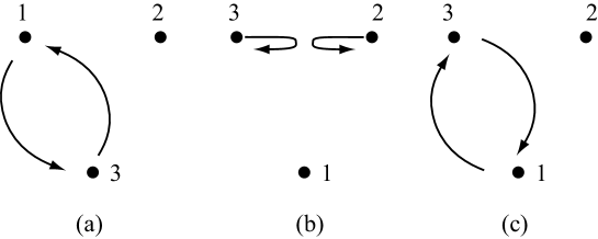
Figure 1: Implementation of a one-qubit gate. Numbers 1, 2 and 3 show the positions of vortices. (a) Vortices at positions 1 and 3 are exchanged (STEP 1). (b) Vortices at 1 and 2 are put close to each other so that they acquire the dynamical phase (STEP 2). (c) Vortices at 1 and 3 are exchanged again so that the vortices take their initial configuration (STEP 3).

1. Suppose vortices at positions 3 and 1 are exchanged in the counterclockwise sense, as shown in Fig. 1 (a), so that the Majorana operators are transformed as $\gamma_{3}\to\gamma_{1}$ and $\gamma_{1}\to-\gamma_{3}$. Under this transformation, the operator $\alpha$ transforms as

   $$\alpha=\frac{e^{-i\phi}}{2}(\gamma_{1}+i\gamma_{2}) \to \frac{e^{-i\phi}}{2}(-\gamma_{3}+i\gamma_{2})$$

   $$= -\frac{e^{-i\phi}}{2}(\alpha\alpha^{\dagger}\beta+\alpha^{\dagger}\alpha\beta)$$

   $$+\frac{e^{-i\phi}}{2}(\alpha e^{i\phi}-\alpha^{\dagger}e^{-i\phi})$$

   Transformations of the operators $\alpha^{\dagger},\alpha\alpha^{\dagger}\beta$ and $\alpha^{\dagger}\alpha\beta$ under this exchange are also obtained and summarized as

   $$\left(\begin{array}[]{c}\alpha\\ \alpha^{\dagger}\alpha\beta\\ \alpha\alpha^{\dagger}\beta\\ \alpha^{\dagger}\end{array}\right)\to m_{31}\left(\begin{array}[]{c}\alpha\\ \alpha^{\dagger}\alpha\beta\\ \alpha\alpha^{\dagger}\beta\\ \alpha^{\dagger}\end{array}\right)$$ (27)

   where

   $$m_{31}=\frac{1}{2}\left(\begin{array}[]{cccc}1&-e^{-i\phi}&-e^{-i\phi}&-e^{-2i\phi}\\ e^{i\phi}&1&-1&e^{-i\phi}\\ e^{i\phi}&-1&1&e^{-i\phi}\\ -e^{2i\phi}&-e^{i\phi}&-e^{i\phi}&1\end{array}\right)$$ (28)

2. Vortices at 1 and 2 are put close to each other, as shown in Fig. 1 (b), so that $J_{12}$ is appreciably large. Now both the ground state and the excited states acquire nontrivial phases. The transformation matrix is

   $$m_{z}=\left(\begin{array}[]{cccc}e^{-i\eta}&0&0&0\\ 0&e^{i\eta}&0&0\\ 0&0&e^{-i\eta}&0\\ 0&0&0&e^{i\eta}\end{array}\right).$$ (29)

3. Subsequently, vortices at 3 and 1 are exchanged in clockwise sense as shown in Fig. 1 (c), which introduces $m_{31}^{-1}$.

The above three steps result in a transformation matrix

$$m_{31}^{-1}m_{z}m_{31}$$ (34)

$$= \left(\begin{array}[]{cccc}\cos\eta&-ie^{-i\phi}\sin\eta&0&0\\ -ie^{i\phi}\sin\eta&\cos\eta&0&0\\ 0&0&\cos\eta&ie^{-i\phi}\sin\eta\\ 0&0&ie^{i\phi}\sin\eta&\cos\eta\end{array}\right).$$

This result shows that the qubit basis vectors $|0\rangle=\alpha|0)_{1}|0)_{2}|0)_{3}$ and $|1\rangle=\alpha^{\dagger}\alpha\beta|0)_{1}|0)_{2}|0)_{3}$ are continuously transformed. This statement remains true if another set of the qubit basis vectors, $|0\rangle=\alpha\alpha^{\dagger}\beta|0)_{1}|0)_{2}|0)_{3}$ and $|1\rangle=\alpha^{\dagger}|0)_{1}|0)_{2}|0)_{3}$, are chosen.

It is instructive to implement the Hadamard gate

$$U_{\rm H}=\frac{1}{\sqrt{2}}\left(\begin{array}[]{cc}1&1\\ 1&-1\end{array}\right)$$

with our scheme. We use $|0\rangle=\alpha|0)_{1}|0)_{2}|0)_{3}$ and $|1\rangle=\alpha^{\dagger}\alpha\beta|0)_{1}|0)_{2}|0)_{3}$ as the qubit basis. Then the upper-left block of the matrix (LABEL:eq:gate) has relevance. Let us write

$$M(\eta,\phi)=\left(\begin{array}[]{cc}\cos\eta&-ie^{-i\phi}\sin\eta\\ -ie^{i\phi}\sin\eta&\cos\eta\end{array}\right).$$ (36)

Then we easily verify the product $M(\frac{\pi}{4},-\frac{\pi}{2})M(\frac{\pi}{2},0)$ implements the Hadamard gate up to an overall phase.

Qubit operations are also possible by exchanging vortices at 2 and 3, instead of vortices at 1 and 2. It is also easy to verify that a similar qubit construction and qubit operations are possible if the qubit basis states are made of even fermion number states. The sequence of operations given in Fig. 1, in this case, results in the matrix (LABEL:eq:gate), although $m_{31}$ takes a different form from the odd fermion case (28).

It has been shown so far that a continuous family of 1-qubit operations can be implemented by adding a third Majorana fermion to a pair of Majorana fermions.

IV Two-Qubit Gates

Finally, we show that our qubits satisfy the universality criterion by demonstrating that two-qubit gates can be implemented within the current proposal. We first note that the third Majorana fermion is required only to implement single-qubit gates and plays no role if it is far remote from the first and the second Majorana fermions. Let us first consider the braiding proposed in I01 . Let $\gamma_{1}$ and $\gamma_{2}$ ($\gamma^{\prime}_{1}$ and $\gamma^{\prime}_{2}$) be the Majorana fermion operators associated with qubit 1 (2), where an index associated with the second qubit is denoted with a prime. Let the initial state of qubits 1 and 2 be $\alpha\alpha^{\prime}|0\rangle$, where

$$\alpha=\frac{1}{2}(\gamma_{1}+i\gamma_{2}),\ \alpha^{\prime}=\frac{1}{2}(\gamma^{\prime}_{1}+i\gamma^{\prime}_{2})$$

and we write $|0)_{1}|0)_{2}|0)_{1^{\prime}},|0)_{2^{\prime}}$ as $|0)$ to simplify the notation. Ivanov [I01 ] attempted to create an entangled state $\frac{1}{\sqrt{2}}(|0\rangle|0\rangle+|1\rangle|1\rangle)$ by braiding of Majorana fermions. Let us exchange Majorana fermions 1 and 1’ in the counterclockwise sense. The state then transforms as

$$\alpha\alpha^{\prime}|0)\to\frac{1}{2}(\alpha\alpha^{\prime}+\alpha^{\dagger}\alpha^{\prime\dagger}-\alpha\alpha^{\dagger}\alpha^{\prime}\alpha^{\prime\dagger}+\alpha^{\dagger}\alpha\alpha^{\prime\dagger}\alpha^{\prime})|0),$$

which is certainly an entangled state. However, this state is different from the state

$$\frac{1}{\sqrt{2}}(|0\rangle|0\rangle+|1\rangle|1\rangle)=\frac{1}{\sqrt{2}}(\alpha\alpha^{\prime}+\alpha^{\dagger}\alpha\alpha^{\prime\dagger}\alpha^{\prime})|0),$$ (37)

for example, to be implemented

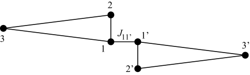
Figure 2: Two-qubit system. Physical quantities associated with the second qubit are denoted with a prime. The coupling strength between Majorana fermions 1 and 1’ is denoted as $J_{11^{\prime}}$, for example.

Now we would like to propose an alternative operation to implement the state (37). We first let Majorana fermion $\gamma_{1}$ of qubit 1 and Majorana fermion $\gamma^{\prime}_{1}$ of qubit 2 come closer so that they interact with each other. The relevant interaction Hamiltonian is

$$iJ_{11^{\prime}}\gamma_{1}\gamma_{1^{\prime}}=iJ_{11^{\prime}}(\alpha+\alpha^{\dagger})(\alpha^{\prime}+\alpha^{\prime\dagger}).$$ (38)

The interaction strengths are arranged to satisfy

$$|J_{12}|,|J_{1^{\prime}2^{\prime}}|\gg|J_{11^{\prime}}|$$ (39)

and

$$|J_{11^{\prime}}|\gg|J_{12}-J_{1^{\prime}2^{\prime}}|.$$ (40)

It follows from the condition (39) that the state $\alpha\alpha^{\prime}|0)$ has no time evolution since $J_{11^{\prime}}$ is negligible compared to $J_{12}+J_{1^{\prime}2^{\prime}}$. In contrast, there is an oscillation between two states $\alpha\alpha^{\prime\dagger}\alpha^{\prime}|0)$ and $\alpha^{\dagger}\alpha\alpha^{\prime}|0)$ since it follows from the condition (40) that $|J_{12}-J_{1^{\prime}2^{\prime}}|$ is negligible compared to $J_{11^{\prime}}$. Now we are ready to outline how to generate a state like (38).

1. We first prepare the state $\alpha\alpha^{\prime}|0)$.

2. Apply $M(\pi/2,\pi/2)$ of Eq. (36) on the second qubit to generate a state $\alpha\alpha^{\prime\dagger}\alpha^{\prime}|0)$.

3. Introduce $J_{11^{\prime}}$ coupling to transform the state into

   $$\frac{1}{\sqrt{2}}(\alpha\alpha^{\prime\dagger}\alpha^{\prime}+\alpha^{\dagger}\alpha\alpha^{\prime})|0).$$

4. Apply $M(\pi/2,\pi/2)$ again on the second qubit to obtain the entangled state

   $$\frac{1}{\sqrt{2}}(-\alpha\alpha^{\prime}+\alpha^{\dagger}\alpha\alpha^{\prime\dagger}\alpha^{\prime})|0)$$ (41)

   as promised.

We have dropped the operators $\beta$ and $\beta^{\prime}$ which appear in the intermediate state.

There is practically no change in the state (41) due to the condition (39) once this state is created. Qubits 1 and 2 may be widely separated for further stabilization.

V Conclusion

In conclusion, we have proposed new qubit construction in topological quantum computing, in which Majorana fermions trapped in a two-dimensional $p$-wave superfluid are employed. A single qubit is constructed out of three Majorana fermions. An arbitrary one-qubit gate can be implemented by a combination of the braiding of the vortices (and hence the Majorana fermions) and the dynamical phase change. Entangling operation required for two-qubit gate implementation is shown be realizable in a similar manner.

Introducing a dynamical phase in TQC might seem to be a flaw in an otherwise perfect quantum computation scheme. It should be noted, however, that a brading in mathematics, which requires exact exchange of positions of Majorana fermions, is never possible to realize physically. Exchange of positions in reality always involve an imperfection.

References

(1) D. A. Ivanov, Phys. Rev. Lett. 86, 268 (2001).
(2) C. Zhang, S. Tewari, and S. Das Sarma, Phys. Rev. Lett.
99, 220502 (2007).
(3) S. B. Chung and S.-C. Zhang, arXiv:0907.4394 (2009).
(4) V. Gurarie and L. Radzihovsky. Ann. Phys. 322,
2 (2007).
(5) T. Mizushima, M. Ichioka, and K. Machida, Phys. Rev. Lett.
101, 150409 (2008).
(6) C. Nayak, S. H. Simon, A. Stern, M. Freedman, and
S. Das Sarma, Rev. Mod. Phys. 80, 1083 (2008).
(7) T. Mizushima and K. Machida, private communication.