Abstract

We consider a gravitational field in steady state galaxy models of two kinds. Some of them are axisymmetrical and others are triaxial. Equipotentials and potential law are given separately in accordance to Kutuzov and Ossipkov (1980a). The relatively simple potential law is based on Kuzmin–Malasidze model (1969). Two kinds of models contain four and five structural parameters respectively. One composite model is suggested as well. Some examples of trajectories are calculated in these models. The simplest method to describe orbits is drawing their projections on coordinate planes. However it needs a great amount of calculation and makes troubles in an interpretation of information. In the case of axisymmetrical models a motion in co-moving meridional plane (with cylindrical coordinates R, z) is considered as a common way. In the case of triaxial models one can use three different co-moving planes passing through moving star and corresponding coordinate axis. We describe models in sections 2–4, calculated orbits are discussed in section 5.

Key words: galaxies: kinematics and dynamics – galaxies: structure – methods: numerical

1 Introduction

In recent years trajectories of stars in various models of the gravitational field of the galaxies have been constructed intensively. We intend to clear up how do orbit characteristics depend on model properties. Similar investigation was fulfilled by Kutuzov & Ossipkov (1992), where box eccentricities and maximal elevation of 70 orbits of open clusters in three models were compared. Here we investigate relation of the orbit properties with variation of the properties of different in principle models — axially symmetric and triaxial. This work continues our research (Kutuzov & Raspopova 2008).

There is a great variety of models in literature. We mention just few of them. Ossipkov (1997) has performed an exhaustive analysis of fourth-order (quaternary) equipotentials of general form with some parameters for systems with rotational symmetry.

Dynamical models of triaxial elliptical galaxies were constructed by Arnold et al. (1994) using Stäckel potential for calculating the dependence velocity field of the model on the shapes of orbits. Merritt and Fridman (1996) showed essential role of the stochastic orbits in triaxial gravitational field with central density cusps. For similar model Merritt and Valluri (1996) found that central point mass designed to represent nuclear black hole causes stochastic orbits to diffuse through phase space. Kutuzov (1997) suggested the model with eighth-order equipotentials, providing triaxial mass distribution.

Here we use simpler triaxial fourth-order equipotentials of special form (Kutuzov 1998). One of the parameters, responsible for the triaxial shape, is specified in the form of a variable in such a way that equipotentials asymptotically tend to spheres, thus, the natural requirement for the models of finite mass is satisfied. A rarely used property, according to which the dependence of the coefficients in the equation of level surfaces on the parameters of the family does not change the order of the equation, is employed. In the special case a biaxial disk embedded in the halo occurs.

2 Family of axially symmetric models

All the quantities are dimensionless. The change to dimensional quantities is fulfilled by multiplication ones by the corresponding scaling parameters. Basic ones are units of length, potential and mass

$$\hat{r},\quad\hat{\Phi},\quad\hat{\cal M}=\hat{r}\hat{\Phi}/G,$$

where $G$ is gravitational constant.

At first, we consider axisymmetrical models. The potential law is specified analytically with free parameters and the one independent variable $\xi$. The only argument $\xi$ is a function of coordinates

$$\varphi=\varphi(\xi)\,,\quad\xi^{2}=f(R,\;z)\,.$$ (1)

The variable $\xi$ is the equipotential parameter that changes from one equipotential to another, determining their family. Putting $\xi=$ const formula (1) gives equation of a fixed equipotential.

Equipotentials and potential law are given separately in accordance to Kutuzov & Ossipkov (1980a). Ten models being the special cases of mentioned family were listed by Kutuzov & Ossipkov (1980b). These models were suggested earlier by P. P. Parenago (1950, 1952), G. M. Idlis (1961), G. G. Kuzmin (1953, 1956), A. Toomre (1963), H. Plummer (1911), M. Miyamoto and R. Nagai (1975), M. Hénon (1959), G. G. Kuzmin and Ü.-I. K. Veltmann (1972). Euipotentials, constructed there, were generalized later (Kutuzov 1989). According to (1), equipotentials are determined by the function $f(R,\;z)$. Two-parametric family of equipotentials was suggested (Kutuzov 1989)as follows

$$\xi^{2}=r^{2}+2\mu(1-\varepsilon)(q-\varepsilon)\,,\quad r^{2}=R^{2}+z^{2}\,,\quad q=\sqrt{\varepsilon^{2}+z^{2}}\,.$$ (2)

Quantities $\varepsilon,\;\mu$ are structural parameters of the model

$$0\leq\varepsilon\leq 1\;,\qquad 0\leq\mu<\infty\;.$$

The first term on the right-hand of equation describes the spherical shape of equipotentials at infinity. The second term causes to a disk component in the model when $\varepsilon\to 0$. These equipotentials coincide with the ones of the model of Miyamoto & Nagai (1975) for $\mu=1$. Let us compare our equipotentials with the model of Satoh (1980). We perform the dimensional potential of that model to

$$\Phi(\xi)=\frac{G\cal M}{\hat{r}\sqrt{1-\varepsilon^{2}+\xi^{2}}},\quad\xi^{2}=r^{2}+2(1-\varepsilon)(q-\varepsilon).$$

It is obvious that these equipotentials are a special case of our ones (2) when $\mu=1$. For $\varepsilon=1$ the model is spherical, potential has discontinuity in the center, where $\xi=0$. System degenerates into mass point with Kepler potential.

We take another potential law

$$\varphi(\xi)=\frac{\alpha}{\beta+\sqrt{1+\varkappa\xi^{2}}}\,\qquad\beta=\alpha-1\,,$$ (3)

that coincides in the plane $z=0$ with Kuzmin–Malasidze law(1969). Thus accepted family of the models has four structural dimensionless parameters $\varepsilon,\>\mu,\>\alpha,\>\varkappa$. It gives great opportunities for modeling of the various galaxies and star clusters. The potential is normed so that in the center $\varphi(0)=1$.

Asymptotics of the potential allows us to find the expression for the dimensionless mass of the model

$${\cal M}=\frac{\alpha}{\sqrt{\varkappa}}\,.$$

When $\varepsilon=1$ or $\mu=0$ the force field is spherically symmetrical, because $\xi=r$ according to (2). In the case of $\varepsilon=0$ the force has a discontinuity in the $z=0$ plane, as $q=|z|$. This determines the existence of an infinitely thin circular disk, imbedded into continuous halo; dimensionless mass of the disk is equal $\mu$ (Kutuzov 1989).

3 Family of triaxial models

We still take potential in the form of (1), but now its argument $\xi$ is the function of three Cartesian coordinates $x,y,z$ (with the origin at center of mass)

$$\xi^{2}=g(x,y,z)\;.$$

Clearly, the addition of $\xi$ to the list of arguments, i.e. the representation $f(x,y,z,\xi)$, does not change the order of the equipotential equation relative to the $x,y,z$ coordinates.

Let the function $f(x,y,z,\xi)$ consist of three terms

$$\xi^{2}=r^{2}+2\,\mu(1-\varepsilon)\,(q-\varepsilon)+\tau(\xi)\,s^{2}\;,\quad 0\leq\xi<\infty\;.$$ (4)

Here,

$$r^{2}\equiv x^{2}+y^{2}+z^{2}\;,\quad q\equiv\sqrt{\varepsilon^{2}+z^{2}}\;,$$

$$s^{2}\equiv y^{2}-x^{2}\begin{cases}\geq 0,&|x|\leq|y|\,;\\ <0,&|x|>|y|\,.\end{cases}$$

The new expression differs from (2) by his third term, that is responsible for the triaxial shape. Coefficient $\tau$ is assumed to be a function of $\xi$. Let us call it the triaxiality parameter. Sometimes it is convenient to express $\tau$ in terms of some bounded function $\chi(\xi)$ that is proportial to it

$$\tau(\xi)=(1-\varepsilon)\,\chi(\xi)\;.$$ (5)

For $\varepsilon=1$ $r^{2}$ remains on the right side of eq. (4), which implies that the model is spherical. But now equality $\mu=0$ does not mean transfer to the spherical model, because the triaxiality parameter might be not equal zero. Below we’ll discuss function $\tau(\xi)$ in details. We only note here that for $\tau\equiv 0$ the model ceases to be triaxial, including models with rotational symmetry (2) as a special case. Note also that the parameter $\xi$ is expressed in terms of the $x,y,z$ coordinates implicitly. To calculate it from the coordinates, we must solve eq. (4) using eq. (5), for example, by successive approximations by assuming initially that $\tau=0$.

The equation of equipotential (4) has fourth order with respect to coordinates. It gives the second-order equation in equatorial plane

$$\xi^{2}=(1-\tau)\,x^{2}+(1+\tau)\,y^{2}\;.$$ (6)

The section of the equipotential by the equatorial plane is an ellipse for $|\tau|<1$. Equation (6) yields the following expressions for the semi-major and semi-minor axes of the ellipse

$$a^{2}=\frac{\xi^{2}}{1-\tau(\xi)}\;,\quad b^{2}=\frac{\xi^{2}}{1+\tau(\xi)}\;.$$ (7)

If $0\leqslant\tau(\xi)<1$, the two axes are real, and $b\leqslant\xi\leqslant a$ .

Kutuzov (1998) suggested the following constraints on the triaxiality parameter $\tau(\xi)$. It is desirable (but not necessary) that, as one approaches the system’s center, the ellipse (6) changes to a circumference that would shrink to a point

$$\tau(0)=0\;.$$ (8)

For the potential to become spherically symmetric at infinity, the following limit must exist

$$\lim_{\xi\to\infty}\tau(\xi)=0\;.$$ (9)

In this case, $\tau$ must tend to zero as some negative power of $\xi$. The third term on the right side of (4) will then have an order that is less than 2. Since the second term has only the first order in $z$, the first term, which always has order 2, dominates.

In order that the semimajor axis $a$ of the ellipse (6) be no smaller than its semiminor axis $b$, and that both axes remain bounded for a finite $\xi$, we assume that

$$0\leqslant\tau(\xi)<1\;.$$ (10)

The equipotentials of the family must not intersect (and touch) each other. This requires that the axes $a$ and $b$ be monotonically increasing functions of $\xi$

$$a^{\prime}(\xi)>0\;,\qquad b^{\prime}(\xi)>0\;.$$

The prime denotes differentiation with respect to $\xi^{2}$. Taking into account (7), we obtain differential inequalities which the triaxiality parameter must satisfy

$$\xi^{2}\tau^{\prime}(\xi)-\tau(\xi)+1>0,\quad\xi^{2}\tau^{\prime}(\xi)-\tau(\xi)-1<0.$$

Here are three examples of the function $\chi(\xi)$, that satisfy the necessary conditions

$$\chi_{1}(\xi)=\displaystyle\frac{A_{1}}{1+\xi^{2}}\;,\quad\chi_{2}(\xi)=\displaystyle\frac{A_{2}\xi^{2}}{1+\xi^{4}}\;,\quad\chi_{3}(\xi)=\displaystyle\frac{A_{3}\xi}{1+\xi^{2}}\;,$$ (11)

with the following constraint on the positive parameters

$$A_{i}<\frac{1}{1-\varepsilon},\quad i=1,2,3\,.$$

The first function does not satisfy constraint (8), so that the model is also triaxial in the central region. The function $\tau$ is defined in terms of $\chi$ by formula (5). The coefficients $A_{i}$ allow us to make the triaxiality parameter $\tau$ arbitrarily small.

We still use expression (3) for the potential law. In the case when the coefficients $A_{i}$ are equal zero, the model coincides with axially symmetric one entirely.

A circular velocity has no sence in triaxial model. So we introduce quasi-curcular velocity, that just characterizes the gravitational field

$$W^{2}=-R\>\left[\frac{\partial\psi(R,\;z)}{\partial R}\right]_{z=0},\quad\psi(R,\;z)=\left.\varphi(\xi)\right|_{x=y},\quad R=\sqrt{x^{2}+y^{2}}.$$ (12)

4 Composite models

Two families of the models considered in sections 2, 3 give us favorable opportunities for modeling the various galaxies and star clusters. But we get more flexible instrument if we use superposition of the models of these families. We define the set of parameters as

$$p_{n}=\{\varepsilon_{n},\,\mu_{n},\,\alpha_{n},\,\varkappa_{n},A_{i}^{(n)}\}\,,\qquad n=\overline{1,N}.$$

here $i$ — number of the selected expression in (11). Then N–component model of the gravitational field is the weighted sum of the potentials (3), (4)

$$\varphi=\sum_{n=1}^{N}w_{n}\varphi_{n}(\xi_{n})\,,\qquad\sum_{n=1}^{N}w_{n}=1\,,$$

where $w_{n}$ are assigned normalized weight coefficients. Mass densities are summed up in just the same way. For example, if we take $N=2$, $\varepsilon_{1}=0$, $\varepsilon_{2}>0$, $A_{k}^{(1)}=A_{k}^{(2)}=0$, and all the other model parameters in both components we retain unchanged then we have five free parameters, including $w_{1}$. In such a model force relief field might involve crater either do not involve or involve crater with central peak.

5 Investigation and discussion of orbits

5.0. We solve Cauchy problem to construct the trajectory of the star. The system of ordinary differential equations of the second order is

$$\mathbf{\ddot{r}}=\nabla\varphi(\xi)\,.$$

Here $\mathbf{r}$ is a position vector of the star with respect to the center. Initial conditions are given for arbitrary moment of time $t_{0}$:

$$\mathbf{r}(t_{0})=\mathbf{r}_{0},\qquad\mathbf{v}(t_{0})=\mathbf{v}_{0},$$

where ${\bf v}=\dot{\mathbf{r}}$ — velocity vector of the star.

We use dimensionless time (and all the other functions and variables). Interval of integration is characterized by number of crossings the plane $z=0$ or $y=0$.

System of ordinary differential equations of the second order is transformed to the form of equations of the first order in a usual way and is solved numerically. We used Merson’s method and Dormand-Prince one with variable time step (Hairer, Nersett, Wanner 1990) in order to control specified accuracy. We have chosen these methods, as they supplied rather small relative error for the integral of energy.

5.1. Energy $E$ and $z$-component of the angular momentum $L_{z}$ are the integrals of motion for the axisymmetrical model (Ogorodnikov 1958)

$$E=\varphi(\xi)-\frac{1}{2}(v_{m}^{2}+v_{\theta}^{2})\,,\quad L_{z}=Rv_{\theta}\,,\quad v_{m}^{2}=v_{R}^{2}+v_{z}^{2}\,.$$

Here $v_{R}$, $v_{\theta}$, $v_{z}$ are the velocity components in cylindrical coordinates, $v_{m}$ is a meridional velocity, $E$ is the total energy with the opposite sign. Using $z$-component of the angular momentum one can write the equations of motion as a system of five equations of the first order (Kutuzov & Ossipkov 1981):

$$\left\{\begin{aligned} \dot{R}&=v_{R}\,,&\displaystyle{\dot{v}}_{R}&=L_{z}^{2}/R^{3}+F_{R}\,,\cr\dot{\theta}&=L_{z}/R^{2}\,,&&\cr\dot{z}&=v_{z}\,,&\displaystyle{\dot{v}}_{z}&=F_{z}\,,\end{aligned}\right.$$ (13)

$F_{R}$, $F_{z}$ are the components of force $\mathbf{F}$ per unit mass.

We calculate trajectories of the stars either with the initial zero full velocity or with the initial zero meridional velocity. That stars we call falling ones. Some periodic orbits were found (Fig. 1). Fig. 1a shows the orbit of the star, falling from the contour of zero-velocity curve. Fig. 1b presents the orbit of the falling star, with the initial zero full velocity.

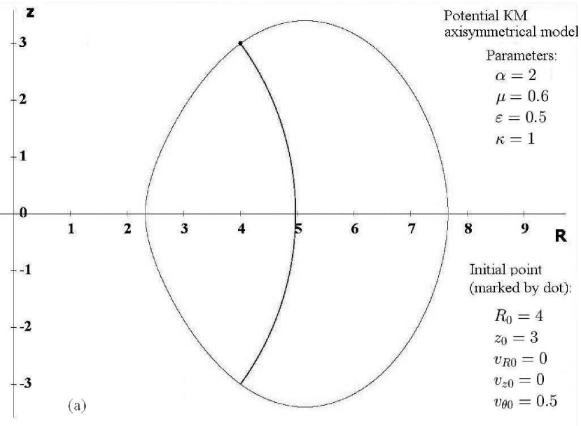
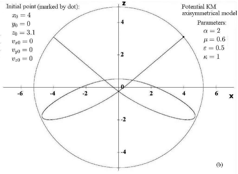
Figure 1: Periodic orbits in axisymmetrical model: the trajectory of the falling star inside the area bounded by the zero-velocity curve.

If we assign small perturbations in the initial phase coordinates these orbits conserve the form, filling the tube with varying width, which includes initial periodic parent orbit (Fig. 2a). We form perturbations such a way so to make star to begin its motion from the equipotential passing through the initial point of the parent orbit. As we see in Fig. 2b the orbit does not conserve its form and does not include parent orbit if perturbations are rather large. We have similar result while varying velocity components. Notice that trajectory does not reach equipotential curve in the half-plane $z<0$ in Fig. 1b, 2a .

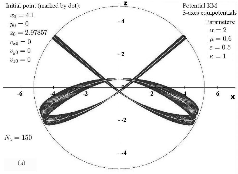
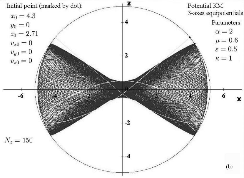
Figure 2: Effect of varying initial conditions for periodic orbit in Fig.1b.

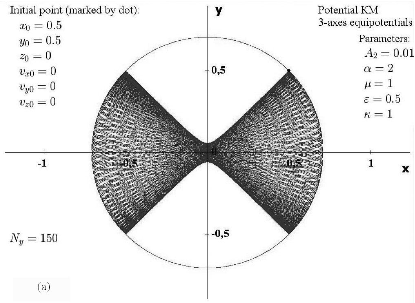
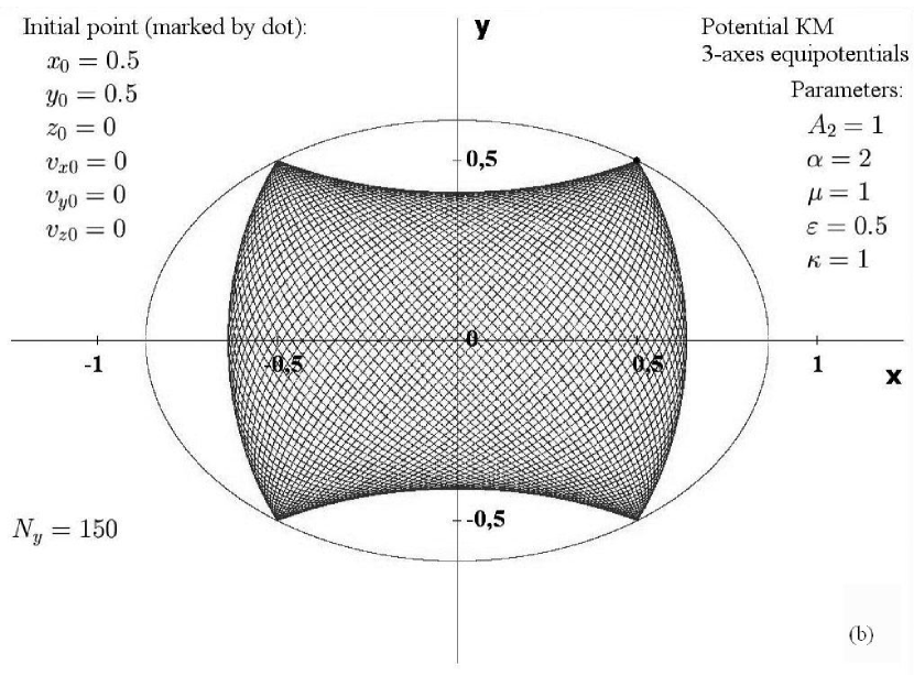
Figure 3: Variations of the coefficient $A_{2}$ in triaxility parameter $\tau$.

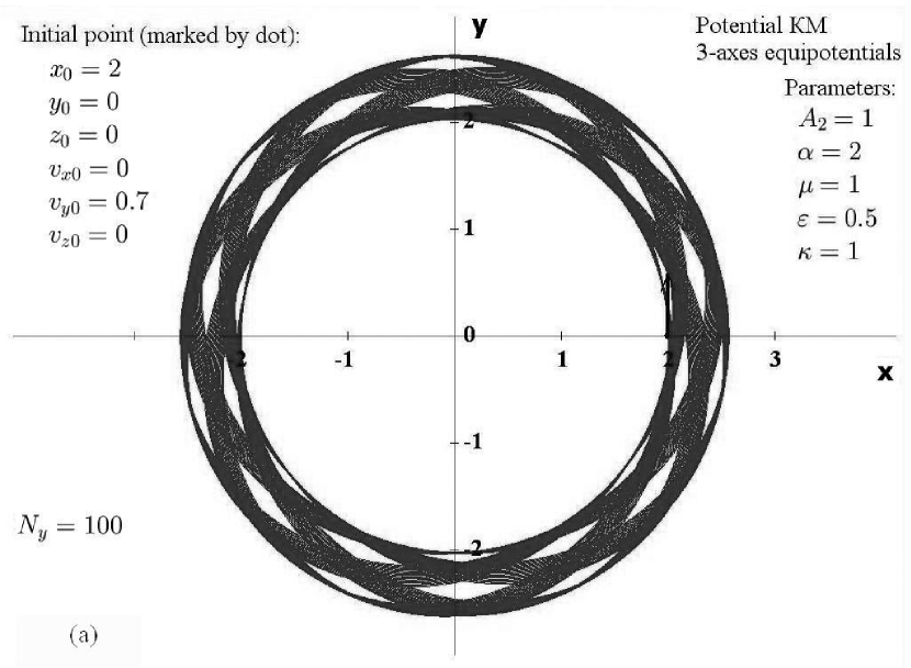
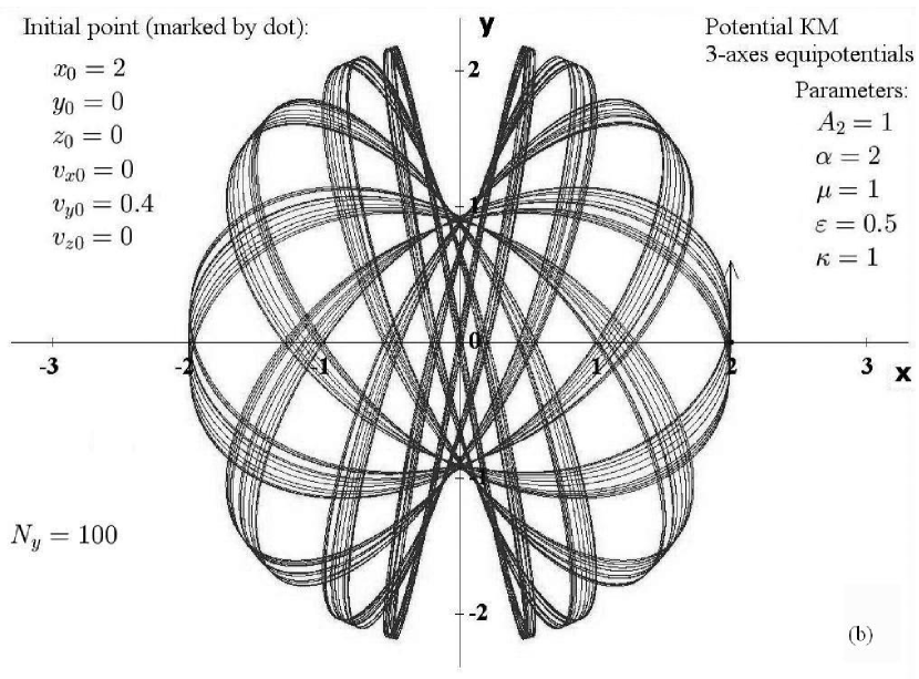
Figure 4: Loop and box orbits in triaxial model

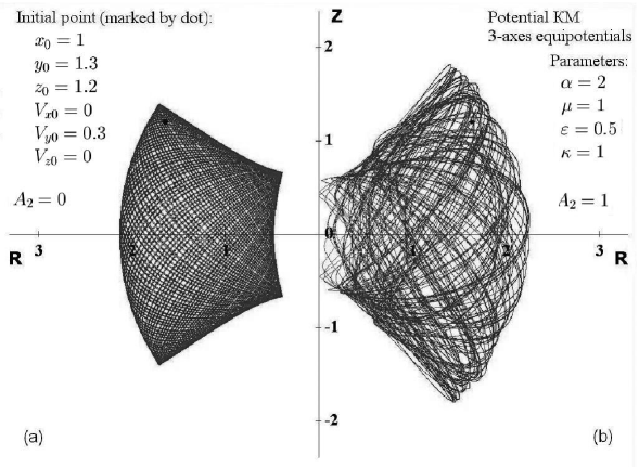
Figure 5: Two trajectories in their co-moving planes. (a) — in axysimmetrical model; (b) — in triaxial model. Iniatial positions and velocity components are the same for both trajectories

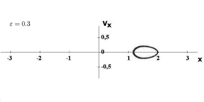
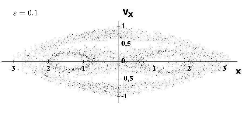
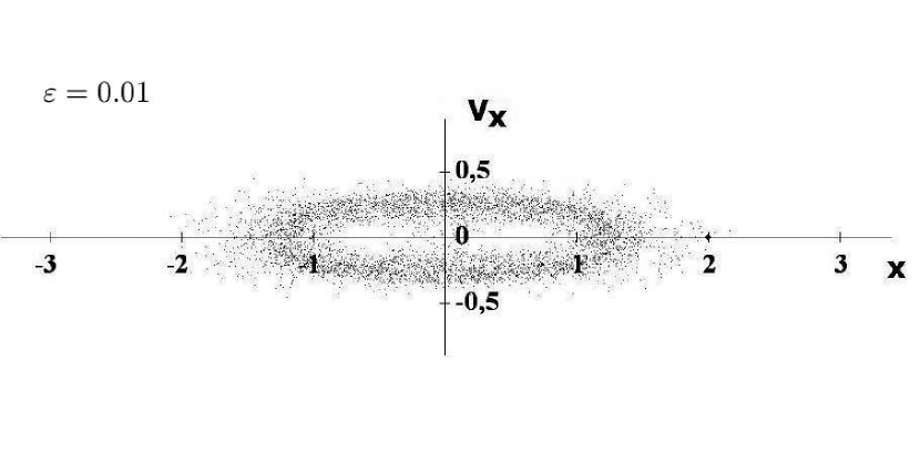
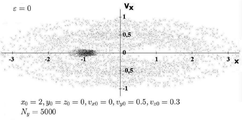
Figure 6: Surfaces of section for orbits in triaxial models with various flattening. Initial positions are the same for all orbits, values of parameters are the same too, except $\varepsilon$. $N_{y}$ is the number of crossing the plane $y=0$ with positive $v_{y}$.

5.2. We consider orbits in triaxial model further. Trajectories of a star, falling from the same initial point in the fields with various triaxiality parameters, are shown in Fig. 3.

It’s also interesting to consider trajectory when the inial point lies on the $x$-axis, while initial velocity is directed along the $y$-axis. For the axially symmetric model the trajectory lies inside the area bounded by circular orbit if the initial velocity (its nonzero component $v_{y}$) is smaller than circular velocity at the initial point. It lies outside if the initial velocity is larger than circular one. The same situation is observed for the triaxial model (Fig. 4) in respect of the quasi-circular velocity (12).

It’s convenient to study orbits in the co-moving meridional plane for the axisymmetrical potentials (Fig. 5a). We construct orbits in the analogical plane for the triaxial model (Fig. 5b). Bounds of the orbit become more “dishevelled”.

By analogy with Poincaré surfaces of section (Binney & Tremaine 1987) we can construct six diagrams. The first pair of them has axes $x,\;\dot{x}$. Points with these coordinates are plotted at the moments when $y=0,\;\dot{y}>0$ or $z=0,\;\dot{z}>0$ respectively. Other diagrams could be obtained by cyclic permutation of coordinates. Surfaces of section $(x,v_{x})$ when $y=0,\;v_{y}>0$ for the triaxial orbits are shown in Fig. 6. Calculations are made for the models with various values of $\varepsilon$. We remind that the value $\varepsilon=1$ means a spherical model and $\varepsilon=0$ means a model with embedded sharp disk. Obviously a stochasticity grows with a flattening.

We plan to continue the calculation and analysis of orbits in various orbits, describing real galaxies.

Acknowledgments

This work was partly supported by the RFBR (Grant 08-02-00361).

References

- Arnold R., de Zeeuw P. T., Hunter C., 1994, MNRAS, 271, 924.
- Binney J., Tremaine S., Galactic Dynamics, Princeton: Princeton Univ. Press, 1987.
- Hairer E., Nersett S. P., Wanner G., Solving Ordinary Differential Equations, Moscow: Mir, 1990 (in Russian).
- Hénon M., 1959, Ann. d’astrophys., 22, 2, 126.
- Idlis G. M., 1961, Proceedings of the Astrophysical Institute of the Kazakh SSR cademy of Sciences. Vol. 1 (in Russian).
- Kutuzov S. A., 1989, Vestnik Leningr. Univ., No 8, 79 (in Russian).
- Kutuzov S. A., 1997, in Structure & Evolution of Stellar Systems, eds. T. A. Agekian, A. A. Müllari, V. V. Orlov, Saint Petersburg: St. Petersburg Univ. Press, 133.
- Kutuzov S. A., 1998, Astronomy Letters, 24, No 5, 645.
- Kutuzov S. A., Ossipkov L. P., 1980a, AZh, 57, 28 (in Russian).
- Kutuzov S. A., Ossipkov L. P., 1980b, Bull. Abastumani obs., No 52, 93 (in Russian).
- Kutuzov S. A., Ossipkov L. P., 1992, Astronomical and geodesic investigation: Motion of the natural and artificial celestial bodies, Ekaterinburgh: Ural Univ. Press, 16 (in Russian).
- Kutuzov S. A., Raspopova N. V., 2008, Vestnik SPb Univ., No 1, 32 (in Russian).
- Kuzmin G. G., 1953, Izvestia AN ESSR, 2, 368 (in Russian).
- Kuzmin G. G., 1956, AZh, 33, 1, 27 (in Russian).
- Kuzmin G. G., Malasidze G. A., 1969, Publ. Tartu Astrophys. Obs., 38, 181 (in Russian).
- Kuzmin G. G., Veltmann Ü.-I. K., 1972, Publ. Tartu Astrophys. Obs., 40, 281 (in Russian).
- Merritt D., Fridman T., 1996, ApJ, 460, 136.
- Merritt D., Valluri M., 1996, ApJ, 471, 82.
- Miyamoto M., Nagai R., 1975, Publ. Astron. Soc. Japan, 27, 533.
- Ogorodnikov K. F., Dinamika zvezdnykh sistem (Dynamics of Stellar Systems), Moscow: Fizmatgiz, 1958 (in Russian; Engl. transl. by J.B.Sykes: London: Pergamon Press, 1965).
- Ossipkov L. P., 1997, Astronomy Letters, 23 , No 3, 385 .
- Parenago P. P., 1950, AZh, 27, 6, 329 (in Russian).
- Parenago P. P., 1952, AZh, 29, 3, 245 (in Russian).
- Plummer H. C., 1911, MNRAS, 71, 460.
- Satoh C., 1980, Publs Astron. Soc. Japan, 32, No 1, 41.
- Toomre A., 1963, ApJ, 138, 2, 385.