Anisotropic Fermi liquid theory of the ultra cold fermionic polar molecules: Landau parameters and collective modes

Abstract

We study the Fermi liquid properties of the cold atomic dipolar Fermi gases with the explicit dipolar anisotropy using perturbative approaches. Due to the explicit dipolar anisotropy, Fermi surfaces exhibit distortions of the $d_{r^{2}-3z^{2}}$-type in three dimensions and of the $d_{x^{2}-y^{2}}$-type in two dimensions. The fermion self-energy, effective mass, and Fermi velocity develop the same anisotropy at the Hartree-Fock level proportional to the interaction strength. The Landau interaction parameters in the isotropic Fermi liquids become the tri-diagonal Landau interaction matrices in the dipolar Fermi liquids which renormalize thermodynamic susceptibilities. With large dipolar interaction strength, the Fermi surface collapses along directions perpendicular to the dipole orientation. The dynamic collective zero sound modes exhibit an anisotropic dispersion with the largest sound velocity propagating along the polar directions. Similarly, the longitudinal $p$-wave channel spin mode becomes a propagating mode with an anisotropic dispersion in multi-component dipolar systems.

I Introduction

The Fermi liquid theory is one of the most important paradigms in contemporary condensed matter physics, which sets up the fundamental framework to understand interacting fermion systems leggett1975 ; baym1991 . The most prominent feature of the Fermi liquid theory is the existence of the Fermi surface and the long-lived low energy fermionic quasi-particles around the Fermi surface. The interaction effects, which may not be weak, can be conveniently described by a set of phenomenological Landau interaction parameters $F_{l}$ in different partial wave channels characterized by the orbital angular momentum number $l$. Physical susceptibilities, including compressibility, specific heat, and spin susceptibility receive important but still finite renormalizations by the Landau interactions. Furthermore, Fermi liquid states possess collective excitations such as the zero sound mode whose restoring force is provided by Landau interactions.

When Landau interaction parameters are negative and large enough, Fermi liquid states may become unstable toward Fermi surface distortions named the Pomeranchuk instabilities pomeranchuk1959 . The most familiar example is ferromagnetism lying in the $s$-wave spin channel. High partial wave channel instabilities in both density and spin channels have been studied extensively in recent years oganesyan2001 ; halboth2000 ; Nilsson2006 ; kee2003 ; wu2004 ; wu2007 ; varma2005 ; hirsch1990 . Another well-known, but of little practical relevance, is the Kohn-Luttinger superconductivity driven by interactions in the high angular momentum channels kohn1965 . The density Pomeranchuk instabilities in high partial channels exhibit anisotropic Fermi surface distortions which are electronic version of the nematic liquid crystal states oganesyan2001 ; halboth2000 ; Nilsson2006 ; kee2003 . Non-$s$-wave spin channel Pomeranchuk instabilities are essentially “unconventional magnetism”, in analogy to unconventional superconductivity. They include both isotropic and anisotropic phases dubbed $\alpha$ and $\beta$-phases as the counterparts of ³He-$B$ (isotropic) and $A$ (anisotropic) phases wu2004 ; wu2007 ; varma2005 ; hirsch1990 ; oganesyan2001 , respectively leggett1975 .

On the other hand, the rapid experimental progress of cold atomic physics provides an exciting opportunity to study quantum many-body systems with electric and magnetic dipolar interactions ospelkaus2008 ; ni2008 ; griesmaier2005 ; mcclelland2006 ; lu2009 . When electric dipole moments are aligned by the external field, dipolar interaction decays as $1/r^{3}$, and thus is long-ranged in three dimensions (3D) but remains short-ranged in two dimensions (2D). More importantly, the most prominent feature of dipolar interaction is its spatial anisotropy which possess the $d_{z^{2}-3r^{2}}$ anisotropy in 3D and the $d_{x^{2}-y^{2}}$ anisotropy in 2D, respectively. Considerable progress has been made in studying exotic properties in anisotropic condensations of the dipolar bosonic systems as reviewed in Refs koch2008 ; lahaye2009 ; lahaye2009a ; menotti2007a .

Furthermore, dipolar fermionic systems provide another exciting opportunity to study exotic anisotropic many-body physics of fermions, including anisotropic Fermi liquid states and Cooper paring states. Physical observable should exhibit the same anisotropy accordingly such as the shape of the Fermi surface sogo2008 ; miyakawa2008 ; chang2009. Anisotropic Cooper pairing and Wigner crystallization of dipolar Fermi gases has been theoretically investigated baranov2002 ; baranov2004 ; baranov2008a ; baranov2008b ; bruun2008 . Recently, Fregoso et al. fregoso2009 studied the biaxial nematic instability in the dipolar Fermi gases as the $d$-wave channel Pomeranchuk instability, and generalized the Landau interaction parameters to the tridiagonal Landau interaction matrices.

Anticipating a great deal of experimental and theoretical activity in the near future in polar molecular and atomic interacting fermionic systems, we have provided in this article a comprehensive Landau Fermi liquid theory for polar interactions including the full effects of anisotropy. The explicit dimensionless perturbation parameter is the ratio between the characteristic dipolar interaction energy and the Fermi energy. The standard textbook isotropic Fermi liquid theory is generalized into the anisotropic version which exhibits many different features of both single-fermion and collective properties. Our theory is a leading-order perturbative theory in the polar interaction coupling constant, which is equivalent to a Hartree-Fock approximation of the interaction. We expect our theory to be quantitatively accurate in the weak coupling regime, but the qualitative aspects of our theory, e.g. the effect of anisotropy on the Fermi liquid parameters, should be generally valid. Our work only considers the explicit anisotropy due to the alignment of the molecular electric dipolar moment. The spontaneous anisotropic phase as a ferro-nematic state of the dilute magnetic dipolar Fermi gases has been recently studied by Fregoso et al. in Ref. fregoso2009a

In Sect. II, the Fourier transforms of the dipolar interactions in 3D and 2D are summarized, which nicely exhibit the $d_{r^{2}-3z^{2}}$ symmetry and the $d_{x^{2}-y^{2}}$ symmetry, respectively. The anisotropic interactions result in anisotropic Fermi surfaces. The angular dependence of Fermi wavevectors, Fermi velocities, and effective masses are presented in Sect. III. All of them exhibit the same isotropy proportional to the the dipolar interaction strength at the leading order.

Because the dipolar interaction mixes different partial wave channels, the Landau interaction parameters in isotropic systems becomes Landau interaction matrices. In Sect. IV, the Landau interaction matrices in 3D calculated in Ref. fregoso2009 are reviewed, and those in 2D are constructed Fortunately due to the $d_{z^{2}-3r^{2}}$-symmetry of the dipolar interaction, the mixing turns out to result in the tri-diagonal matrix. between $l$ and $l\pm 2$ in 3D. The thermodynamic susceptibilities would be renormalized by the generalized Landau matrices as will be discussed in Sect. V. In this section, we will also explore the thermodynamic instability, where Fermi surface collapses along directions perpendicular to the dipole orientation.

In Sect. VI, we study the 3D collective modes in both the density and spin channels, respectively, focusing on the anisotropy effect. The dynamic collective zero sound mode exhibits an anisotropic dispersion. The sound velocity is largest if the propagation direction is along the north and south poles, and becomes softened as the propagation deviates from them. For directions close to the equator of the Fermi surface, the zero sound cannot propagate. The spin-channel collective modes do not exist in the $s$-wave spin wave channel. Nevertheless, well-defined propagating collective modes appears in the longitudinal $p$-wave spin channel, which has not been observed in condensed matter systems before.

Conclusions and outlooks are made in Sect. VII.

II The dipolar interaction in three and two dimensions

The most prominent feature of the dipolar interaction is its spatial anisotropy, i.e., it depends on not only the distance between two dipoles but also the angles between their relative vectors and dipole orientations. In the case that all the dipoles are orientated along the external electric field $\vec{E}$ set as the $z$-axis, the dipolar interaction between dipoles at $\vec{r}_{1}$ and $\vec{r}_{2}$ reads

$$V_{3D}(\vec{r}_{1}-\vec{r}_{2}) = {d^{2}\over{|\vec{r}_{1}-\vec{r}_{2}|^{3}}}(1-3\cos^{2}\theta_{\vec{r}_{1}-\vec{r}_{2}})$$ (1)

$$= -{2d^{2}\over{|\vec{r}_{1}-\vec{r}_{2}|^{3}}}P_{2}(\cos\theta_{\vec{r}_{1}-\vec{r}_{2}}),$$

where $\theta_{\vec{r}_{1}-\vec{r}_{2}}$ is the angle between $\vec{r}_{1}-\vec{r}_{2}$ and the $\vec{E}$-field; $d$ is the electric dipole moment. The anisotropy exhibits in the angular dependence of the $V_{3D}$ with the form of the second Legendre polynomial. $V_{3D}$ is repulsive for $\bar{\theta}_{0}<\theta_{\vec{r}_{1}-\vec{r}_{2}}<\pi-\bar{\theta}_{0}$, and attractive otherwise, where

$$\bar{\theta}_{0}=\cos^{-1}\frac{1}{\sqrt{3}}\approx 55^{\circ}.$$ (2)

If the spatial locations of dipoles are confined in a two dimensional plane, and the $\vec{E}$-field is set in the $xz$-plane with an angle of $\theta_{0}$ relative to the plane as depicted in Fig. 1, then Eq. 1 reduces to

$$V_{2D}(\vec{r_{1}}-\vec{r}_{2},\theta_{0})={d^{2}\over{|\vec{r}_{1}-\vec{r}_{2}|^{3}}}(1-3\sin^{2}\theta_{0}\cos^{2}\phi)$$

$$={d^{2}\over{|\vec{r}_{1}-\vec{r}_{2}|^{3}}}\big{\{}P_{2}(\cos\theta_{0})-\frac{3}{2}\sin^{2}\theta_{0}\cos 2\phi\big{\}},$$ (3)

where $\phi$ is the azimuthal angle relative to the $x$-axis. Eq. 3 is decomposed into the isotropic component and an anisotropic $d$-wave component, whose relative weight is tunable by varying the parameter angle $\theta_{0}$. If $\vec{E}$ is perpendicular to the plane, i.e. $\theta_{0}=0$, $V_{2D}$ is isotropic and repulsive. On the other hand, at $\theta_{0}=\bar{\theta}_{0}$, $V_{2D}$ is purely anisotropic with the $d$-wave form factor $\cos 2\phi$. As the external electric field is tilted, i.e., $\theta_{0}$ varies from $0$ to $\frac{\pi}{2}$, the 2D dipolar interaction gradually changes from an isotropic repulsive to an attractive one at large value of $\theta_{0}$.

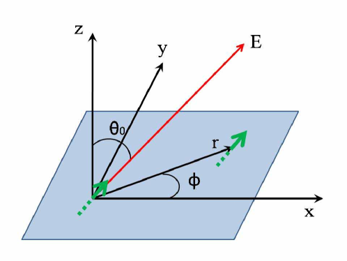
Figure 1: Schematic sketch of a 2D dipolar system. The external electric field $\vec{E}$ controls the dipole orientation and thus the dipolar interaction.

The anisotropies in the Fourier transform of dipolar interactions in both 3D and 2D exhibit in their dependencies on momentum orientations. In order to handle both the long range part and the short distance divergence of the dipolar interactions, we introduce a small distance cutoff $\epsilon$ beyond which the dipolar interactions Eq. 1 and Eq. 3 are valid, and a large distance cutoff $R$. $\epsilon$ can be chosen, say, one order larger than the size of the dipolar molecule and $R$ is the radius of the system.

II.1 Fourier transform of the 3D dipolar interaction

For the 3D dipolar interaction, its Fourier transform can be performed as

$$V_{3D}(\vec{q}) = 8\pi d^{2}\big{\{}\frac{j_{1}(q\epsilon)}{q\epsilon}-\frac{j_{1}(qR)}{qR}\big{\}}P_{2}(\cos\theta_{\vec{q}})$$ (4)

$$\longrightarrow \frac{8\pi d^{2}}{3}P_{2}(\cos\theta_{\vec{q}}),$$

at $q\epsilon\rightarrow 0$ and $qR\rightarrow\infty$. Its angular dependence is the second Legendre polynomial of momentum direction inherited from the real space form of Eq. 1; $j_{1}(x)$ is the first order spherical Bessel function with the asymptotic behavior $j_{1}(x)\rightarrow\frac{x}{3}$ as $x\rightarrow 0$; and $j_{1}(x)\rightarrow\frac{1}{x}\sin(x-\frac{\pi}{2})$ as $x\rightarrow\infty$.

Eq. 4 does not depend on the magnitude of $q$ after the limits of $q\epsilon\rightarrow 0$ and $qR\rightarrow+\infty$ are taken because of the spatial integral over $1/r^{3}$ renders the result dimensionless. At $\vec{q}=0$, $V_{3D}(\vec{q}=0)=0$ arising from the fact that the spatial average of the 3D dipolar interaction is zero. However, $V_{3D}(\vec{q})$ is not analytic as $\vec{q}\rightarrow 0$ in the limit of $R\rightarrow+\infty$ due to the angular variation. In fact, the smallest value of $qR$ is at the order of $O(1)$, this non-analyticity even exist for large but finite value of $R$.

An interesting feature of the above Fourier transforms is that $V_{3D}(\vec{q})$ is most positive when $\vec{q}$ is along the $z$-axis, but most negative when $\vec{q}$ is in the equator plane, which is just opposite to the case of $V_{3D}(\vec{r})$ in real space. This can be intuitively understood as follows. Considering a dipole density wave propagating along the $z$-axis, the wave fronts (equal phase lines) are perpendicular to the dipole orientation, thus the interaction energy is repulsive. On the other hand, if the dipole density wavevector lies in the equator, then the wave fronts are parallel to the dipole orientation which renders the interaction negative.

II.2 Fourier transform of the 2D dipolar interaction

In two dimensions, the Fourier transform of Eq. 3 is more subtle, which can be expressed as

$$V_{2D}(\vec{q},\theta_{0}) = 2\pi d^{2}P_{2}(\cos\theta_{0})\Big{\{}\frac{1}{\epsilon}-\frac{J_{0}(qR)}{R}$$ (5)

$$+ q\big{[}J_{1}(q\epsilon)-J_{1}(qR)\big{]}-qI_{2}(q\epsilon,qR)\Big{\}}$$

$$+ \pi d^{2}\sin^{2}\theta_{0}\cos 2\phi_{q}~{}q\Big{\{}3\big{[}\frac{J_{2}(qR)}{qR}-\frac{J_{2}(q\epsilon)}{q\epsilon}\big{]}$$

$$- \big{[}J_{3}(qR)-J_{3}(q\epsilon)\big{]}+I_{2}(q\epsilon,qR)\Big{\}},$$

where $J_{0,1,2}(x)$ are the Bessel functions of the 1st, 2nd, and 3rd orders, respectively; $I_{2}$ is the integral defined as

$$I_{2}(q\epsilon,qR)=\int^{qR}_{q\epsilon}dxJ_{2}(x),$$ (6)

and $I_{2}(0,+\infty)=1$. In the regular limit of $q\epsilon\rightarrow 0$ and $qR\rightarrow+\infty$, the complicated form of Eq. 5 can be simplified into

$$V_{2D}(\vec{q},\theta_{0}) = 2\pi d^{2}P_{2}(\cos\theta_{0})(\frac{1}{\epsilon}-q)$$ (7)

$$+ \pi d^{2}\sin^{2}\theta_{0}~{}q\cos 2\phi_{q}.$$

In particular, at $\theta_{0}=\bar{\theta}_{0}$, Eq. 7 is entirely anisotropic,

$$V_{2D}(\vec{q},\theta_{0}=\bar{\theta}_{0})={2\pi d^{2}\over{3}}q\cos 2\phi_{q},$$ (8)

as one can see from the real space interaction in Eq. 3. Eq. 7 even holds in the long wavelength limit $qR\rightarrow O(1)$. On the other hand, for the short wavelength limit $x=q\epsilon$ at the order of $O(1)$, additional terms should be added into Eq. 7 as

$$\Delta V_{2D}(\vec{q}\rightarrow 0,\theta_{0}) = 2\pi d^{2}P_{2}(\cos\theta_{0})\frac{1}{\epsilon}[xJ_{1}(x)+xI_{2}(0,x)]$$ (9)

$$+ \pi d^{2}\sin^{2}\theta_{0}\cos\phi_{q}\frac{1}{\epsilon}[3J_{2}(x)+xJ_{3}(x)$$

$$- xI_{2}(0,x)].$$

In the dilute limit, where the Fermi wavevector $k_{f}$ satisfies $k_{f}\epsilon\ll 1$, we only need to use $q$ up to the order of $k_{f}$. Thus in the sections below, we shall use Eq. 7 as the 2D Fourier transform of our dipolar interaction.

The anisotropic component of $V_{2D}(\vec{q})$ (second term of Eq. 7) has a similar feature to the 3D case, which is repulsive along the $x$-axis but negative along $y$-axis. Notice that there is also an isotropic component for $V_{2D}$ which can be either positive or negative depending on the external parameter $\theta_{0}$. Therefore, in momentum space, the dipolar interaction in 2D contains both $s$ and $d$-wave components, while it only has a $d$-wave symmetry in 3D.

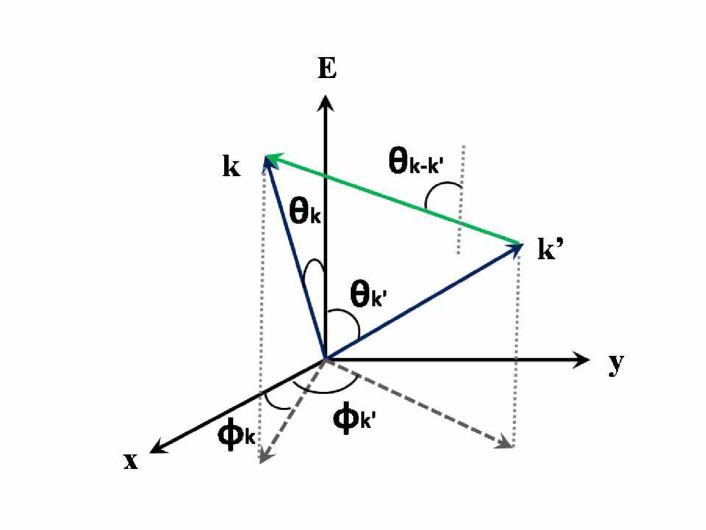
Figure 2: The dipole moments polarized by the external $\vec{E}$-field are along the $z$-axis. The polar and azimuthal angles of $\vec{k}$ and $\vec{k}^{\prime}$ are denoted by $\theta_{k(k^{\prime})}$ and $\phi_{k(k^{\prime})}$, respectively. $\theta_{\vec{k}-\vec{k}^{\prime}}$ is the polar angle of the vector difference of $\vec{k}-\vec{k}^{\prime}$ but not the angle between $\vec{k}$ and $\vec{k}^{\prime}$.

III Hartree-Fock Self-energy and Fermi Surface Deformation

The anisotropy of the dipolar interaction exhibits in the fermion self-energy at the Hartree-Fock level, which results in anisotropic Fermi surface distortions as studied in Refs fregoso2009 ; sogo2008 ; miyakawa2008 . A convenient dimensionless parameter to describe the interaction strength is defined in 3D and 2D as fregoso2009

$$\lambda_{3D} = \frac{E_{int}^{3D}}{E^{3D}_{k_{f0}}}=\frac{d^{2}mk_{f_{0}}^{3D}}{3\pi^{2}\hbar^{2}},$$

$$\lambda_{2D} = \frac{E_{int}^{3D}}{E^{2D}_{k_{f0}}}=\frac{d^{2}mk_{f_{0}}^{2D}}{4\pi^{3/2}\hbar^{2}},$$ (10)

where $k_{f0}^{3D,2D}$ are the non-interacting Fermi wavevectors in 3D and 2D, respectively; $E_{int}$ is the average dipolar interaction and $E_{k_{f0}}^{3D,2D}=\frac{\hbar^{2}(k^{3D,2D}_{f0})^{2}}{2m}$ are the kinetic energies at the Fermi surface in the absence of interaction. Since that $\lambda_{3D}$ and $\lambda_{2D}$ are at the same order, we will not distinguish them but use $\lambda=\lambda_{3D}$ for both 2D and 3D. In this section, we shall evaluate the Hartree-Fock self-energy in 2D and 3D perturbatively at the linear order of $\lambda$ from which the Fermi surface distortion will be determined. We will see that both the Hartree-Fock self-energies and Fermi surface distortions possess the same symmetries inherited from the corresponding interactions.

III.1 Anisotropic Hartree-Fock self-energy in 3D

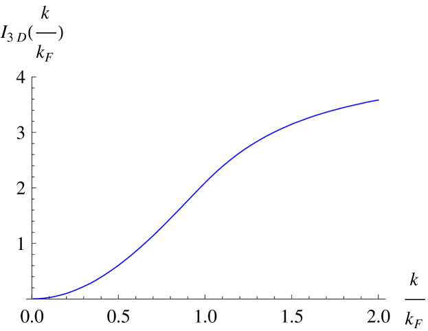
Figure 3: The dimensionless $k$-dependent function $I_{3D}(\frac{k}{k_{f}})$ of the 3D Hartree-Fock self-energy in Eq. 13.

We first consider the situation in 3D, the Hartree-Fock self-energy can be expressed as

$$\Sigma^{HF}_{3D}(\vec{k}) = \frac{1}{V}\sum_{k^{\prime}}\big{\{}V_{3D}(\vec{q}=0)-V_{3D}(\vec{k}-\vec{k^{\prime}})\big{\}}n_{\vec{k^{\prime}}}$$ (11)

$$= -\frac{8\pi d^{2}}{3V}\sum_{k^{\prime}}P_{2}(\cos\theta_{\vec{k}-\vec{k}^{\prime}})n_{\vec{k}^{\prime}}$$

$$= -\frac{8\pi d^{2}}{3}\int_{k^{\prime}<k_{f0}}\frac{d^{3}k^{\prime}}{(2\pi)^{3}}P_{2}(\cos\theta_{\vec{k}-\vec{k}^{\prime}})$$

where $n_{\vec{k}}$ is the Fermi occupation number; the Hartree contribution goes to zero. In Eq. 11, the leading contribution of the anisotropy to $\Sigma^{HF}(\vec{k})$ comes from the interaction. The effect from the Fermi surface distortion is at a higher order of $\lambda$, and thus is neglected, thus we will take the Fermi wavevector in Eq. 11 as that of zero dipolar interaction $k_{f0}^{3D}$. $\theta_{\vec{k}-\vec{k^{\prime}}}$ is the angle between the momentum transfer $\vec{k}-\vec{k^{\prime}}$ and $\vec{E}$, which satisfies

$$\cos\theta_{\vec{k}-\vec{k}^{\prime}} = \frac{(\vec{k}-\vec{k}^{\prime})\cdot\hat{E}}{|\vec{k}-\vec{k}^{\prime}|}$$ (12)

Please notice that $\theta_{\vec{k}-\vec{k^{\prime}}}$ is not the angle between $\vec{k}$ and $\vec{k^{\prime}}$ (see Fig. 2).

This Hartree-Fock self-energy can be evaluated analytically as

$$\Sigma^{HF}_{3D}(\vec{k})=-2\lambda E_{k_{f0}}^{3D}P_{2}(\cos\theta_{k})\ I_{3D}({k\over k_{f_{0}}^{3D}}),$$ (13)

where $E_{k_{f0}}=\hbar^{2}k_{f0}^{2}/2m$ and

$$I_{3D}(x) = \frac{\pi}{12}\Big{\{}3x^{2}+8-{3\over x^{2}}+\frac{3(1-x^{2})^{3}}{2x^{3}}\ln|\frac{1+x}{1-x}|\Big{\}}$$

is a monotonically increasing function as depicted in Fig. 3. This form agrees with the self-energy calculated for the 3D dipolar Fermi gases in Ref. fregoso2009 . Right on the Fermi surface,

$$\Sigma_{3D}^{HF}(k=k_{f0}^{3D}) = -\frac{4\pi}{3}\lambda E_{k_{f0}}^{3D}P_{2}(\cos\theta_{k}).$$ (15)

Naturally Eq. 13 exhibits the $d$-wave form factor $P_{2}(\cos\theta_{k})$. We shall see more examples below where the physical quantities possess the symmetry originated from the dipolar nature.

III.2 Anisotropic Hartree-Fock self-energy in 2D

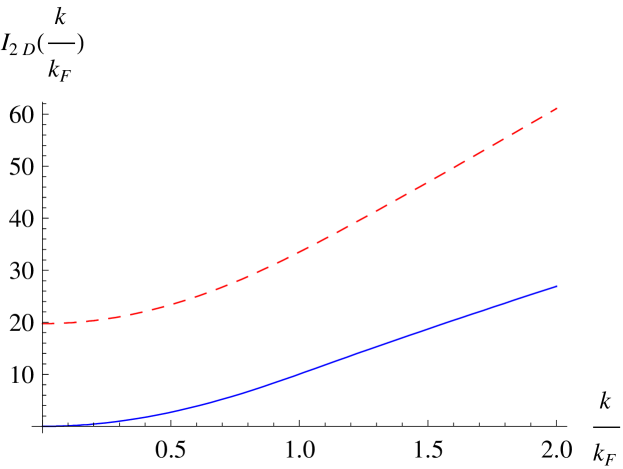
Figure 4: The $k$-dependent components of the 2D HF self-energies in 2D. The solid (blue) and dashed (red) curves represent the dimensionless functions $I_{2D}^{ani}(k/k_{f})$ and $I_{2D}^{iso}(k/k_{f})$ defined in Eq. 16.

Similarly, for 2D system, the HF self-energy is evaluated as

$$\Sigma^{HF}_{2D}(\vec{k},\theta_{0}) = \lambda E_{k_{f0}}^{2D}\Big{\{}P_{2}(\cos\theta_{0})\ I_{2D}^{iso}\Big{(}\frac{k}{k_{f0}^{2D}}\Big{)}$$ (16)

$$- \sin^{2}\theta_{0}\cos 2\phi_{k}\ I_{2D}^{ani}\Big{(}{k\over k_{f0}^{2D}}\Big{)}\Big{\}},$$

where $k_{f0}^{2D}$ is the Fermi wavevector at zero dipolar interaction and

$$I_{2D}^{iso}(x) = 12\pi\int_{0}^{1}dx^{\prime}x^{\prime}|x+x^{\prime}|E\Big{(}\frac{2\sqrt{xx^{\prime}}}{x+x^{\prime}}\Big{)}$$

$$I_{2D}^{ani}(x) = 2\pi\int_{0}^{1}dx^{\prime}\frac{x^{\prime}|x+x^{\prime}|}{x^{2}}\Big{\{}(x-x^{\prime})^{2}K\Big{(}\frac{2\sqrt{xx^{\prime}}}{x+x^{\prime}}\Big{)}$$ (17)

$$\ \ \ \ \ \ \ \ \ \ \ +\ \ (2x^{2}-x^{\prime 2})E\Big{(}\frac{2\sqrt{xx^{\prime}}}{x+x^{\prime}}\Big{)}\Big{\}}.$$

The functions $K(y)$ and $E(y)$ are the standard complete elliptic integral of the first and second kinds, respectively as

$$K(y) = \int^{\frac{\pi}{2}}_{0}d\alpha\frac{1}{\sqrt{1-y^{2}\sin^{2}\alpha}},$$

$$E(y) = \int^{\frac{\pi}{2}}_{0}d\alpha\sqrt{1-y^{2}\sin^{2}\alpha}.$$ (18)

The behavior of $I_{2D}^{iso}(x)$ and $I_{2D}^{ani}(x)$ are plotted in Fig. 4. Eq. 16 indicates that the self-energy in 2D comprises of an isotropic and an anisotropic terms. The former shifts the chemical potential $\mu$, while the latter distorts the Fermi surface. At $k=k_{f0}^{2D}$, Eq. 16 reduces into

$$\Sigma_{2D}^{HF}(k=k_{f0}^{2D},\phi_{k},\theta_{0})$$

$$= -\lambda E_{k_{f0}}^{2D}\{-\frac{32\pi}{3}P_{2}(\cos\theta_{0})+\frac{16\pi}{5}\sin^{2}\theta_{0}\cos 2\phi_{k}\}.$$

Again, Eq. 16 contains the same angular dependence as the 2D interaction does. Both Eq. 13 and 16 indicate that the Hartree-Fock-self energy changes monotonically with the momentum $k$ in 2D and 3D (Fig. 3 and Fig. 4).

III.3 Hartree-Fock self-energy for two-component dipolar systems

In two-component dipolar systems, the exchange part of the Hartree-Fock self-energy only exists intra-component interaction, and the Hartree part exists in both intra and inter-component interactions. Since the Hartree contribution vanishes in the 3D dipolar systems, the Hartree-Fock self-energy remains the same as in the single-component systems. In the 2D dipolar systems, there is an extra contribution from the inter-component Hartree interaction as

$$\Delta\Sigma_{2D}^{HF}=\frac{3\pi^{2}}{k^{2D}_{f0}\epsilon}\lambda E_{k_{f0}}P_{2}(\cos\theta_{0}),$$ (20)

where $\epsilon$ is the 2D phenomenological cutoff constant we discussed before. This extra self-energy contribution is momentum independent and can be offset by an overall shift of the chemical potential.

III.4 Anisotropic Fermi surface distortions

The anisotropic Hartree-Fock self-energy from the dipolar interaction naturally results in anisotropic Fermi surface distortions. With Eq. 13 and 16, we determine the distortions by solving:

$$\epsilon_{HF}(\vec{k}_{f})=\epsilon_{0}(\vec{k}_{f})+\Sigma^{HF}(\vec{k}_{f})=\mu(n,\lambda).$$ (21)

Here, $n$ is the particle density and we recall that $k^{3D}_{f_{0}}$ is the Fermi wavevector for $\lambda=0$. With nonzero $\lambda$, the dependence of $\vec{k}_{f}$ on the polar angle in 3D is solved as

$$\frac{k_{f}^{3D}(\theta_{k})}{k_{f0}^{3D}}=1-\frac{4\pi^{2}}{45}\lambda^{2}+\frac{2\pi}{3}\lambda P_{2}(\cos\theta_{k}).$$ (22)

Similarly, in 2D, the dependence of $\vec{k}$ on the azimuthal angle is solved as

$$\frac{k_{f}^{2D}(\phi_{k},\theta_{0})}{k_{f0}^{2D}} = 1-\frac{16\pi^{2}}{25}\sin^{4}\theta_{0}\lambda^{2}$$ (23)

$$+ \frac{8\pi}{5}\sin^{2}\theta_{0}\lambda\cos 2\phi_{k}.$$

The anisotropic Fermi surface distortions in 2D and 3D show linear dependence on dipolar interaction strength $\lambda$. Due to particle number conservation, there are small shrinking of Fermi momentum in both 2D and 3D at the quadratic order of $\lambda$. Notice that these two equations are correct to the order of $\lambda$. The $\lambda^{2}$ terms appear to conserve particle numbers due to this lowest order Fermi surface deformation. When higher order contribution is considered, anisotropy can also enter in the second order of $\lambda$ and particle conservation will in turn lead to an isotropic $\lambda^{3}$ correction.

We emphasize here again that the results obtained based on Eq. 13 and Eq. 16 are perturbative and are correct for $\lambda\ll 1$, while they provide qualitative features for $\lambda<1$. As a comparison with the variational approach suggested in Ref. miyakawa2008 , we plot the deformed Fermi surface in Fig. 5 for $\lambda=\frac{1}{2\pi}$ in 3D, which corresponds physically to the stability limit of the dipolar system (to be discussed in Sect. V). Our perturbation results give rise a less prolate shape of the Fermi surface than those obtained from the variational approach. Fig.6 shows the same distorted Fermi surfaces in 2D. At $\theta_{0}=0$, the interaction is isotropic and does not deform the Fermi surface. It becomes prolate when $\theta_{0}$ increases. We would like to emphasize that the interaction is most anisotropic at $\theta_{0}=\bar{\theta}_{0}$, though a larger $\theta_{0}$ will stretch the Fermi surface more.

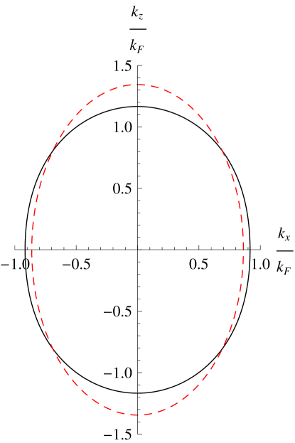
Figure 5: The deformed Fermi surface for $\lambda=\frac{1}{2\pi}$ in the 3D dipolar system obtained by the perturbative (solid) and variational (dashed red) approaches. The external electric field lies along the z axis here.

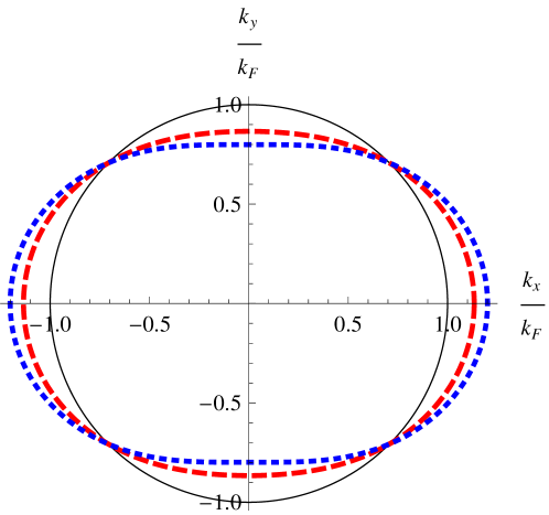
Figure 6: The 2D distorted Fermi surfaces for $\lambda=0.02$. The solid (black), dashed (red) and blue (dotted) curves corresponds to an external electric field configuration at $\theta_{0}$=0, $\bar{\theta}_{0}$ and $\frac{\pi}{2}$ respectively. The electric field is projected to x-axis in this 2D system.

III.5 Anisotropic Fermi velocities and effective masses

The Fermi velocities become anisotropic in both 2D and 3D at non-zero $\lambda$. In comparison to interacting electron systems, the Hartree-Fock contributions to the 2D and 3D dipolar Fermi gases are less singular, i.e.,, the radial derivatives at the Fermi surface remain continuous: the Hartree correction of Fermi velocity is continuous because the Fourier transforms of the dipolar interaction are finite as $\vec{q}\rightarrow 0$. Furthermore, the difference of the Hartree-Fock self-energies for the single component and multi-component dipolar gases is momentum independent, thus the Fermi velocities are the same for both cases and we will not distinguish them in this subsection.

We first consider the 3D case. After taking into account the Hartree-Fock correction, the projections of Fermi velocities along the radial direction $\hat{k}$ and angular direction $\hat{e}_{\theta}$ are defined as $\hat{k}\cdot\vec{v}_{f}^{3D}(\vec{k})$ and $\hat{e}_{\theta}\cdot\vec{v}_{f}^{3D}(\vec{k})$ as

$$\hat{k}\cdot\vec{v}_{f}^{3D}(\vec{k}) = \frac{k_{f}^{3D}(\theta_{k})}{m}+\frac{\partial\Sigma^{HF}_{3D}(k,\theta_{k})}{\partial k},$$

$$\hat{e}_{\theta}\cdot\vec{v}_{f}^{3D}(\theta_{k}) = \frac{\partial\Sigma^{HF}_{3D}(k,\theta_{k})}{k_{f}^{3D}\partial\theta_{k}}.$$ (24)

Taking into account the angular dependence of Fermi wavevector in Eq. 22 and 23, we arrive at the radial and angular Fermi velocities corrections to the linear order of $\lambda$ as

$$\hat{k}_{f}\cdot\vec{v}_{f}^{3D}(\theta_{k}) = \frac{k_{f0}^{3D}}{m}\Big{\{}1-\frac{\pi}{3}\lambda P_{2}(\cos\theta_{k})\Big{\}},$$

$$\hat{e}_{\theta}\cdot\vec{v}_{f}^{3D}(\theta_{k}) = \frac{k_{f0}^{3D}}{m}\pi\lambda\sin 2\theta_{k}.$$ (25)

There are two opposite contributions to $\hat{k}_{f}\cdot\vec{v}_{f}^{3D}$: (1) the Fermi surface deformation, $k_{f}(\theta_{k})$ and (2) the Hartree-Fock self-energy modification. In 3D dipolar system, the latter is stronger and thus the radial Fermi velocity is suppressed at north and south poles but enhanced along the equator of the Fermi surface.

According to Eq. 25, we define the longitudinal and transverse effective masses $m^{*}_{3D,\parallel}$ and $m^{*}_{3D,\perp}$ in 3D as

$$\frac{1}{m^{*}_{3D,\parallel}(\theta_{k})} = \frac{\hat{k}_{f}\cdot\vec{v}_{f}^{3D}(\theta_{k})}{k^{3D}_{f}(\theta_{k})}=\frac{1}{m}\Big{\{}1-\pi\lambda P_{2}(\cos\theta_{k})\Big{\}},$$

$$\frac{1}{m^{*}_{3D,\perp}(\theta_{k})} = \frac{\hat{e}_{\theta_{k}}\cdot\vec{v}_{f}^{3D}(\theta_{k})}{k^{3D}_{f}(\theta_{k})}=\frac{1}{m}\pi\lambda\sin 2\theta_{k}.$$ (26)

For the 2D case, the projections of Fermi velocity in 2D along the radial $\hat{k}$ and the azimuthal angle $\hat{e}_{\phi_{k}}$-directions are calculated as

$$\hat{k}\cdot\vec{v}_{f}^{2D}(\phi_{k},\theta_{0}) = \frac{k_{f0}^{2D}}{m}\Big{\{}1+\lambda\Big{[}4\pi P_{2}(\cos\theta_{0})$$ (27)

$$- \frac{6\pi}{5}\sin^{2}\theta_{0}\cos 2\phi_{k}\Big{]}\Big{\}},$$

$$\hat{e}_{\phi_{k}}\cdot\vec{v}_{f}^{2D}(\phi_{k},\theta_{0}) = \frac{k_{f0}^{2D}}{m}\frac{16\pi}{5}\lambda\sin^{2}\theta_{0}\sin 2\phi_{k}.$$ (28)

For a general value of $\theta_{0}\neq\bar{\theta}_{0}$, there is an additional isotropic renormalization to $v_{f}^{2D}(\phi_{k},\theta_{0})$ in Eq. 27, which comes from the isotropic part of the 2D dipolar interaction.

This means that in 2D, we also have a reduced radial Fermi velocity at $\phi_{k}=0,\pi$, while it is boosted when $\phi_{k}=\pm\frac{\pi}{2}$. Accordingly, similar to the 3D situation, we can also compute the longitudinal and transverse effective masses $m^{*}_{2D,\parallel}$ and $m^{*}_{2D,\perp}$ in 2D as

$$\frac{1}{m^{*}_{2D,\parallel}(\phi_{k},\theta_{0})}$$

$$\ \ \ \ =\frac{1}{m}\Big{\{}1+\lambda\Big{[}4\pi P_{2}(\cos\theta_{0})-\frac{14\pi}{5}\sin^{2}\theta_{0}\cos 2\phi_{k}\Big{]}\Big{\}},$$

$$\frac{1}{m^{*}_{2D,\perp}(\phi_{k},\theta_{0})}=\frac{1}{m}\frac{16\pi}{5}\lambda\sin^{2}\theta_{0}\sin 2\phi_{k}.$$ (29)

III.6 Renormalization of density of states

Now we study the renormalization of the density of states (DOS) at the Fermi surface due to the dipolar interaction at the Hartree-Fock level. We define the 3D differential DOS of the single component $N^{3D}(\Omega_{k})$ in the direction of $\Omega_{k}$ as

$$N^{3D}(\Omega_{k})\frac{d\Omega_{k}}{4\pi} = \frac{k^{3D}_{f}(\theta_{k})d\Omega_{k}}{(2\pi)^{3}v_{f}^{3D}(\theta_{k})}\sqrt{[k^{3D}_{f}(\theta_{k})]^{2}+(\frac{dk_{f}^{3D}}{d\theta_{k}})^{2}}$$ (30)

$$= \frac{mk_{f0}^{3D}}{\hbar(2\pi)^{3}}[1+\frac{5\pi}{3}\lambda P_{2}(\cos\theta_{k})]d\Omega_{k}.$$

At the linear order of $\lambda$, $N^{3D}(\Omega_{k})$ develops the same anisotropy of $P_{2}(\cos\theta)$. The total DOS reads

$$N^{3D}=\int\frac{d\Omega_{k}}{4\pi}N^{3D}(\Omega_{k}),$$ (31)

which does not change at the linear order of $\lambda$ compared to that of the free Fermi gas. This means that the specific heat, which is proportional to the total DOS at the Fermi surface, is not renormalized to the linear order of $\lambda$. In considering the actual area of Fermi surface is enlarged, the correction at higher orders of $\lambda$ should increase the total DOS.

Similarly, we consider the anisotropic case in 2D. The 2D differential DOS of the single component $N^{2D}(\Omega)$ at the Fermi surface along the direction of the azimuthal angle $\phi_{k}$ is defined as

$$N^{2D}(\phi_{k})\frac{d\phi_{k}}{2\pi}=\frac{d\phi_{k}}{(2\pi)^{2}v_{f}^{2D}(\phi_{k})}\sqrt{[k^{2D}_{f}(\phi_{k},\theta_{0})]^{2}+(\frac{dk_{f}^{2D}}{d\phi_{k}})^{2}}=\frac{md\phi_{k}}{(2\pi)^{2}}\Big{\{}1+\lambda\Big{[}-4\pi P_{2}(\cos\theta_{0})+\frac{14\pi}{5}\sin^{2}\theta_{0}\cos 2\phi_{k}\Big{]}\Big{\}},$$

which clearly exhibits the $d$-wave anisotropy. The integrated total DOS at 2D is not changed at the linear order of $\lambda$ either. Similarly, the 2D specific heat is not renormalized to the linear order of $\lambda$.

IV Landau Interactions for the dipolar Fermi liquids

In this section, we construct the Landau Fermi liquid Hamiltonian for the dipolar fermion gas which has also been studied by Fregoso et. al fregoso2009 before. In the isotropic systems, the interaction effects in the Fermi liquid theory are captured by a set of Landau parameters $F_{l}$ in different partial wave channels. In dipolar systems, the anisotropic interaction leads to the mixing of interactions in different partial wave channels, thus we need to generalize the concept of Landau parameters into the Landau matrices.

IV.1 Landau interaction matrix for the single component dipolar gases

In order to have a common reference Fermi surface for different but small values of $\lambda$, we choose it as that of the free fermion gas with the same particle density. Define the variation of the Fermi distribution at momentum $\vec{k}$,

$$\delta n_{\vec{k}}=n_{\vec{k}}-n_{0,k},$$ (33)

where $n_{0}(k)=1-\theta(k-k_{f_{0}}^{3D})$. Assuming a small variation of the fermion distribution $\delta n_{\vec{k}}$ close to the Fermi surface, the ground state energy of the Fermi liquid state changes as

$$\delta E=\sum_{k}\epsilon_{k}\delta n_{k}+\frac{1}{2V}\sum_{\vec{k},\vec{k}^{\prime}}f(\vec{k},\vec{k}^{\prime})\delta n_{\vec{k}}\delta n_{\vec{k}^{\prime}},$$ (34)

where $\vec{k},\vec{k}^{\prime}$ are momenta close to the Fermi surface; $f(\vec{k},\vec{k}^{\prime})$ is the interaction function describing the forward scattering amplitude. $\epsilon_{k}$ includes the bare parabolic dispersion $\epsilon_{k}^{0}$ and the self-energy correction $\Sigma_{HF}(\vec{k})$ which exhibits the $d_{r^{2}-3z^{2}}$ anisotropy. At the Hartree-Fock level, $f(\vec{k},\vec{k}^{\prime})$ is expressed as $f(\vec{k},\vec{k}^{\prime})=V(\vec{q}=0)-V(\vec{k}-\vec{k}^{\prime})$ where the first and second terms are the Hartree and Fock contributions, respectively. Due to the explicit rotational symmetry breaking, $f(\vec{k},\vec{k}^{\prime})$ depends on directions of both $\vec{k}$ and $\vec{k}^{\prime}$, not just the relative angle between $\vec{k}$ and $\vec{k}^{\prime}$ as in isotropic Fermi liquids. For the 3D dipolar system, the classic Hartree term vanishes because the spatial average of the dipolar interaction is zero. However, due to the non-analyticity of the $V_{3D}(\vec{q})$ as $\vec{q}\rightarrow 0$, in the calculation of the zero sound collective excitation in Sect. VI, the dependence of $\vec{q}$ in the Landau interaction needs to be included as

$$\frac{1}{2V}\sum_{\vec{k},\vec{k}^{\prime}}~{}f(\vec{k},\vec{k}^{\prime};\vec{q})~{}n_{\vec{k},\vec{q}}~{}n_{\vec{k},-\vec{q}}.$$ (35)

where $f(\vec{k},\vec{k}^{\prime};\vec{q})=V(\vec{q})-V(\vec{k}-\vec{k}^{\prime})$ and $n_{\vec{k},\vec{q}}=c^{\dagger}_{\vec{k}+\vec{q}}c_{\vec{k}}$.

IV.1.1 3D Landau interactions

In this part, we review the Landau parameter calculation performed in Ref. fregoso2009 . Since quasi-particle excitations are close to the Fermi surface, we integrate out radial direction and obtain the angular distribution. In the 3D system,

$$\delta n(\Omega_{\vec{k}})=\int\frac{k^{2}dk}{(2\pi)^{3}}\delta n_{\vec{k}}.$$ (36)

We expand $\delta n(\Omega_{\vec{k}})$ in terms of the spherical harmonics as

$$\delta n(\Omega_{\vec{k}})=\sum_{lm}Y_{lm}(\Omega_{\vec{k}})\delta n_{lm},$$ (37)

where $Y_{lm}$’s satisfy the normalization convention $\int d\Omega~{}Y^{*}_{lm}(\Omega)Y_{lm}(\Omega)=1$. Due to the anisotropy of the dipolar interaction, its spherical harmonics decomposition becomes

$$f^{3D}(\vec{k},\vec{k}^{\prime})=\sum_{l,l^{\prime};m}\frac{4\pi f_{ll^{\prime};m}^{3D}}{\sqrt{(2l^{+}1)(2l^{\prime}+1)}}Y_{lm}^{*}(\Omega_{k})Y_{l^{\prime}m}(\Omega_{\vec{k}^{\prime}}),$$

(38)

where $f_{ll^{\prime};m}$ remains diagonal for $m$ but couples partial wave channels with $l^{\prime}=l,l\pm 2$. This is a direct result from Wigner-Eckart theorem because the dipolar interaction possesses the symmetry of $d_{r^{2}-3z^{2}}$. The mixing between $l^{\prime}$ and $l$ with $l^{\prime}=l\pm 1$ is forbidden because the dipolar interaction is parity even.

For the 3D systems, the matrix elements $f_{ll^{\prime};m}$ are tridiagonal and have been calculated by Fregoso et al. in Ref. fregoso2009 as

$$f^{3D}_{ll^{\prime};m} = d^{2}\Big{(}a_{lm}^{(1)}\delta_{l,l^{\prime}}+a_{lm}^{(2)}\delta_{l,l^{\prime}-2}+a_{l^{\prime}m}^{(2)}\delta_{l^{\prime},l-2}\Big{)}$$ (39)

where

$$a_{lm}^{(1)} = \frac{4\pi(l^{2}+l-3m^{2})(2l+1)}{l(l+1)(2l+3)(2l-1)},\,$$

$$a_{lm}^{(2)} = -\frac{2\pi}{(l+1)(l+2)(2l+3)}$$ (40)

$$\times \sqrt{[(l+1)^{2}-m^{2}][(l+2)^{2}-m^{2}]},$$

except for the $l=l^{\prime}=m=0$ channel, where we have $f_{00;0}^{3D}(\vec{q})=V_{3D}({\vec{q}})$. Please note that in Eq. 38, we use the standard normalization convention in Ref. leggett1975 ; baym1991 which is different from that in Ref. fregoso2009 , thus the parameters in Eq. 40 are modified accordingly. Sign errors in the original expressions of Ref. fregoso2009 are corrected here. It can be proved that for each $l$, $f^{3D}_{ll^{\prime};m}$’s satisfy the relation that

$$\sum_{m}f_{ll^{\prime}=l;m}^{3D}=0.$$ (41)

We define the average effective radial mass as

$$\bar{m}^{*}_{3D}=\frac{1}{4\pi}\int d\Omega_{k}m^{*}_{3D,\parallel}(\Omega_{k}).$$ (42)

The perturbative result in Eq. III.5 correct to the linear order of $\lambda$ shows $\bar{m}^{*}=m$. Following the standard method to make the Landau matrix dimensionless, we multiply the single component DOS. $F^{3D}_{ll^{\prime};m}=\frac{\bar{m}^{*}}{m}N_{0}^{3D}f^{3D}_{ll^{\prime};m}$ where $N_{0}^{3D}=(mk_{f0}^{3D})/(2\hbar\pi^{2})$ is the DOS of free Fermi gas.

To gain some intuition, we present some values of the low order Landau matrix elements in terms of $\lambda$ as

$$F_{00;0}^{3D}(\Omega_{\vec{q}}) = 4\pi\lambda P_{2}(\cos\theta_{q}),~{}F_{02;0}^{3D}=-\pi\lambda;$$

$$F_{11;0}^{3D} = \frac{18\pi}{5}\lambda;~{}F_{11;\pm 1}=-\frac{9\pi}{5}\lambda;$$

$$F_{22;0}^{3D} = \frac{10\pi}{7}\lambda;~{}F_{22;\pm 1}^{3D}=\frac{5\pi}{7}\lambda;~{}F^{3D}_{22;\pm 2}=-\frac{10\pi}{7}\lambda.$$

$$F^{3D}_{13;0} = -\frac{3\pi}{5}\lambda,F^{3D}_{13;\pm 1}=-\frac{\sqrt{6}\pi}{5}\lambda,$$

$$F^{3D}_{33;0} = \frac{14\pi}{15}\lambda,F^{3D}_{33;\pm 1}=\frac{7\pi}{10}\lambda,F^{3D}_{33;\pm 2}=0,$$

$$F^{3D}_{33;\pm 3} = -\frac{7\pi}{6}\lambda,$$ (43)

IV.1.2 2D Landau interactions

Similarly, in the 2D system, we define the angular distribution $\delta n(\phi_{\vec{k}})$ and its decomposition in the basis of azimuthal harmonics $e^{im\phi_{\vec{k}}}$ as

$$\delta n(\phi_{\vec{k}}) = \int\frac{kdk}{(2\pi)^{2}}\delta n_{\vec{k}}=\sum_{m}e^{im\phi_{\vec{k}}}~{}\delta n_{m}.$$ (44)

The Landau interaction can be represented by a matrix as

$$f^{2D}(\vec{k},\vec{k}^{\prime}) = \sum_{m,m^{\prime}}f_{mm^{\prime}}^{2D}e^{-im\phi_{\vec{k}}}e^{im^{\prime}\phi_{\vec{k}^{\prime}}},$$ (45)

where $f_{mm^{\prime}}^{2D}$ is non-zero when $m^{\prime}=m,m\pm 2$.

We further present our calculation for $f_{mm^{\prime}}$ in 2D which reads

$$f_{mm^{\prime}}^{2D}(\theta_{0})=k_{f0}^{2D}d^{2}\Big{\{}P_{2}(\cos\theta_{0})b_{m}^{(1)}\delta_{m,m^{\prime}}$$

$$\ \ \ \ \ \ \ \ \ \ +\sin^{2}\theta_{0}\Big{(}b_{m}^{(2)}\delta_{m,m^{\prime}-2}+b_{m^{\prime}}^{(2)}\delta_{m^{\prime},m-2}\Big{)}\Big{\}},\ \ \$$ (46)

where

$$b_{m}^{(1)}=-\frac{8}{(2m-1)(2m+1)},$$

$$b_{m}^{(2)}=-\frac{2}{(2m+1)(2m+3)}.$$ (47)

At $\theta_{0}=\bar{\theta}_{0}$ where $P_{2}(\cos\bar{\theta}_{0})=0$, the dipolar interaction is purely anisotropic (see Eq. 8) and the diagonal matrix elements vanish. At this particular angle, the interaction has angular momentum $m=2$, and the matrix element is non-zero only when $m^{\prime}=m\pm 2$ as a result of the Wigner-Eckart theorem.

Similarly, for 2D, we also define the average radial effective mass $\bar{m}^{*}$ which equals to $m$ at the first order of $\lambda$. After multiplying the 2D DOS of the single component Fermi gas, the Landau matrix becomes dimensionless $F^{2D}_{mm^{\prime}}=\frac{\bar{m}^{*}}{m}N_{0}^{2D}f^{2D}_{mm^{\prime}}$ where $N_{0}^{2D}=m/(2\pi\hbar^{2})$ is the DOS of 2D free Fermi gas. Some low order Landau matrix elements are presented in terms of $\lambda$ at the linear order as

$$F_{00}^{2D} = 12\pi P_{2}(\cos\theta_{0})\lambda;~{}~{}F_{11}^{2D}=-4\pi P_{2}(\cos\theta_{0})\lambda;$$

$$F_{22}^{2D} = -\frac{4\pi}{5}P_{2}(\cos\theta_{0})\lambda;$$

$$F_{02}^{2D} = -\pi\sin^{2}\theta_{0}\lambda;~{}~{}F_{1,-1}^{2D}=3\pi\sin^{2}\theta_{0}\lambda.$$ (48)

Eq. 39 and 46 generalize the usual Landau parameters in isotropic Fermi liquid systems to Landau matrices in the dipolar systems. In fact, matrix formalism is a natural generalization as long as anisotropy enters the system. It is the dipolar nature that constrains our Landau matrices to be tridiagonal as shown above.

IV.2 Landau interaction matrix for two-component dipolar Fermi gases

We next consider the Landau interaction matrix a two-component dipolar Fermi gas in 3D. The intra-component Landau interaction contains both Hartree and Fock contributions as in Eq. 35. The inter-component Landau interaction only contains Hartree contribution. The general Landau interaction function is decomposed into density channel response $f_{s}$ and spin-channel response as $f_{a}$

$$f_{\alpha\beta,\gamma\delta}(\vec{k},\vec{k}^{\prime})=f^{s}(\vec{k},\vec{k}^{\prime})\delta_{\alpha\beta}\delta_{\gamma\delta}+f^{a}(\vec{k},\vec{k}^{\prime})\sigma_{\alpha\beta}\sigma_{\gamma\delta},$$ (49)

where $f_{s}$ and $f_{a}$ at the Hartree-Fock level are expressed as

$$f^{s}(\vec{k},\vec{k}^{\prime};\vec{q}) = V(\vec{q})-\frac{1}{2}V(\vec{k}-\vec{k}^{\prime});$$

$$f^{a}(\vec{k},\vec{k}^{\prime};\vec{q}) = -\frac{1}{2}V(\vec{k}-\vec{k}^{\prime}).$$ (50)

Because the DOS at the Fermi surface for the two-component Fermi gases is doubled compared to that of the single-component gases, the Landau matrix elements in the density channel $F^{3D,s}_{ll^{\prime};m}$ and in the spin channel $F^{3D,a}_{ll^{\prime};m}$ at the Hartree-Fock level equal to those $F^{3D}_{ll^{\prime};m}$ defined for the single component case

$$F^{3D,s}_{ll^{\prime};m} = F^{3D,a}_{ll^{\prime};m}=F^{3D}_{ll^{\prime};m},$$

if at least one of $l$ and $l^{\prime}$ are nonzero. The case of $l=l^{\prime}=0$ is special, for 3D we have

$$F^{s}_{00;0}=2F_{00;0};\ \ \ F^{a}_{00;0}=0.$$ (52)

In 2D, a similar conclusion applies at the Hartree-Fock level as

$$F^{2D,s}_{mm^{\prime}}=F^{2D,a}_{mm^{\prime}}=F^{2D}_{mm^{\prime}},$$ (53)

if at least one of $m$ and $m^{\prime}$ are nonzero. For $m=m^{\prime}=0$, we have

$$F^{2D,s,a}_{00}=F^{2D}_{00}\pm\lambda\frac{3\pi^{2}}{\epsilon k_{f}^{2D,0}}P_{2}(\cos\theta_{0}),$$ (54)

where $\epsilon$ is the short range cutoff defined in Sect. II.

IV.3 Landau interaction matrix for $N$-component dipolar Fermi gases

The general $N$-component case is essentially similar in which $N$ arises from the hyperfine multiplets. The $SU(N)$ symmetry is very accurate since the electronic dipolar interaction is independent of the internal hyperfine components. A Fermi liquid theory for the 4-component Fermi gas with $SU(4)$ and $Sp(4)$ symmetry has been constructed by one of us in Ref. wu2003 ; wu2006 , which can be easily generalized to the $N$-component case here. For the convenience of presentation, we first define our convention of the $N^{2}-1$ generators of the $SU(N)$ group

$$[M^{(1)}_{ij}]_{lk}=\delta_{il}\delta_{jk}+\delta_{ik}\delta_{jl}~{}~{}(1\leq i<j\leq n),$$

$$[M^{(2)}_{ij}]_{lk}=-i(\delta_{il}\delta_{jk}-\delta_{ik}\delta_{jl})~{}~{}(1\leq i<j\leq n),$$

$$[M^{3}_{j}]_{lk}=\frac{\mbox{diag}(1,...,1,-(j-1),0,...)}{\sqrt{j(j-1)/2}}~{}(2\leq j\leq n),$$

where $M^{1}$, $M^{2}$ and $M^{3}$ are the $SU(N)$ version of the Pauli matrices of $\sigma_{1}$, $\sigma_{2}$ and $\sigma_{3}$, respectively. Then the $SU(N)$ Fermi liquid Landau interaction can be written as

$$f_{\alpha\beta,\gamma\delta}(\vec{k},\vec{k}^{\prime}) = f^{s}(\vec{k},\vec{k}^{\prime})\delta_{\alpha\beta}\delta_{\gamma\delta}+f^{a}(\vec{k},\vec{k}^{\prime})$$ (56)

$$\times \Big{\{}\sum_{ij}(M^{1}_{ij;\alpha\beta}M^{1}_{ij;\gamma\delta}+M^{2}_{ij;\alpha\beta}M^{2}_{ij;\gamma\delta})$$

$$+ \sum_{i}M^{3}_{i;\alpha\beta}M^{3}_{i;\gamma\delta}\Big{\}},$$

where $f_{s}$ and $f_{a}$ are expressed as

$$f^{s}(\vec{k},\vec{k}^{\prime};\vec{q}) = V(\vec{q})-\frac{1}{N}V(\vec{k}-\vec{k}^{\prime});$$

$$f^{a}(\vec{k},\vec{k}^{\prime};\vec{q}) = -\frac{1}{N}V(\vec{k}-\vec{k}^{\prime}).$$ (57)

Again due to the DOS at the Fermi surface is $N$-times enhanced, the Landau matrix elements for the $N$-component dipolar gas in the density channel $F^{3D,s}_{ll^{\prime};m}$ and in the spin channel $F^{3D,a}_{ll^{\prime};m}$ at the Hartree-Fock level equal to those $F^{3D}_{ll^{\prime};m}$ defined for the single component case as

$$F_{ll^{\prime};m}^{s}=F_{ll^{\prime};m}^{a}=F_{ll^{\prime};m}$$ (58)

when at least one of $l$ and $l^{\prime}$ are nonzero. When $l=l^{\prime}=0$, we have

$$F^{s}_{00;0}=NF_{00;0};\ \ \ F^{a}_{00;0}=0.$$ (59)

In other words, $F^{s}_{00;0}$ has a large $N$-enhancement compared to all of the other Landau matrix elements.

Again, in 2D, a similar conclusion applies at the Hartree-Fock level as

$$F^{2D,s}_{mm^{\prime}}=F^{2D,a}_{mm^{\prime}}=F^{2D}_{mm^{\prime}},$$ (60)

if at least one of $m$ and $m^{\prime}$ are nonzero. For $m=m^{\prime}=0$, we have

$$F^{2D,s}_{00} = F^{2D}_{00}+\lambda(N-1)\frac{3\pi^{2}}{\epsilon k_{f}^{2D,0}}P_{2}(\cos\theta_{0}),$$

$$F^{2D,a}_{00} = F^{2D}_{00}-\lambda\frac{3\pi^{2}}{\epsilon k_{f}^{2D,0}}P_{2}(\cos\theta_{0}).$$ (61)

V Thermodynamic quantities

We next consider the renormalization to the thermodynamic properties from Landau interaction matrices. For the simplicity of presentation, we only consider the single-component dipolar systems here. With slight modifications, the results also apply to the multi-component cases.

V.1 Effective mass and Landau interaction matrix elements

In this subsection, we rederive the effective mass renormalization discussed in Sect. III.5 using Landau matrix formalism. We will see how the Landau parameters in Eq. 39 and 46 enter in the effective masses in 3D and 2D respectively. The formalism below is general for any anisotropic Fermi liquid system (with azimuthal symmetry in 3D).

In Galilean invariant systems, the fermion effective mass renormalization $m^{*}/m=(1+\frac{1}{3}F^{s}_{1})$ is an important result of the isotropic Fermi liquid theory. This results in the same renormalization factor for the DOS at Fermi surface and the specific heat as $C_{FL}/C_{FG}=m^{*}/m$, where $C_{FL}$ and $C_{FG}$ are specific heat for Fermi liquid and ideal Fermi gas, respectively.

For the anisotropic 3D dipolar systems with the Galilean invariance, we present a similar result. The relation connecting effective mass and bare mass still holds for anisotropic interactions landau1957 ; landau1959

$$\frac{\partial\epsilon(\vec{k})}{\partial\vec{k}} = \frac{\vec{k}}{m}+\int\frac{d^{3}\vec{k}^{\prime}}{(2\pi)^{3}}f^{3D}(\vec{k};\vec{k}^{\prime})\frac{\partial n(\epsilon(\vec{k}^{\prime}))}{\partial\vec{k}^{\prime}}.$$ (62)

However, for anisotropic systems, a self-consistent solution to Eq 62 has to be done numerically. To the linear order of $\lambda$, we perform the analytic calculation by approximating $\epsilon(\vec{k}^{\prime})$ in the RHS of Eq. 62 with the free fermion energy as follows. We take the radial derivative of Eq. 62,

$$\frac{1}{m^{*}_{3D,\parallel}(\theta_{k})} = \frac{1}{m}-\frac{N_{0}^{3D}}{m}\int d\Omega_{k^{\prime}}f^{3D}(\vec{k}-\vec{k}^{\prime})(\hat{k}\cdot\hat{k}^{\prime})$$ (63)

$$= \frac{1}{m}\Big{[}1-\tilde{F}_{11,\parallel}(\theta_{k})-\tilde{F}_{13,\parallel}(\theta_{k})\Big{]},$$

where $m^{*}_{3D,\parallel}(\theta_{k})$ is the radial effective mass given in Eq. III.5. $\tilde{F}_{11,\parallel}(\theta_{k})$ and $\tilde{F}_{13,\parallel}(\theta_{k})$ in Eq. 63 are the angular dependent Landau parameters defined as follows

$$\tilde{F}_{11,\parallel}(\theta_{k}) = \frac{4\pi}{3}\sum_{m}\frac{F^{3D}_{11;m}}{3}|Y_{lm}(\theta_{k},0)|^{2}$$ (64)

$$= \frac{18\pi\lambda}{5}P_{2}(\cos\theta_{k}),$$

$$\tilde{F}_{13,\parallel}(\theta_{k}) = \frac{4\pi}{3}\sum_{m=0,\pm 1}\frac{F^{3D}_{13;m}}{\sqrt{21}}Y^{*}_{3m}(\theta_{k},0)Y_{1m}(\theta_{k},0)$$ (65)

$$= \frac{\sqrt{21}\pi}{5}\lambda P_{2}(\cos\theta_{k}).$$

Eq. 63 is a generalization to that of the isotropic case of $m^{*}/m=1+\frac{F^{s}_{1}}{3}$ which can be rewritten as

$$\frac{1}{m^{*}}=\frac{1}{m}-\frac{N_{0}^{3D}}{m}\frac{f_{1}^{s}}{3}.$$ (66)

Thus to the linear order of $\lambda$,

$$\frac{1}{m_{3D,\parallel}^{*}(\theta_{k})}=\frac{1}{m}\big{\{}1-\pi\lambda P_{2}(\cos\theta_{k})\big{\}},$$ (67)

which agrees with Eq. III.5. At the linear order of $\lambda$, as an averaged effect, there should be no specific heat renormalization due to the dipolar interaction.

Parallel analysis can be carried out for the 3D transverse effective mass as

$$\frac{1}{m^{*}_{3D,\perp}(\theta_{k})} = \frac{1}{m}\big{[}\tilde{F}_{11,\perp}(\theta_{k})+\tilde{F}_{13,\perp}(\theta_{k})],$$ (68)

where

$$\tilde{F}_{11,\perp}(\theta_{k}) = \frac{1}{6}\big{(}F_{11;0}^{3D}-\frac{F_{11;1}^{3D}+F_{11;-1}^{3D}}{2}\big{)}\sin 2\theta_{k},$$

$$\tilde{F}_{13,\perp}(\theta_{k}) = -\frac{4\pi}{3}\sqrt{\frac{2}{21}}\Big{[}F_{13;0}^{3D}Y_{11}(\theta_{k},0)Y_{30}(\theta_{k},0)$$ (69)

$$+ \frac{Y_{10}(\theta_{k},0)}{2}\Big{(}Y_{3,-1}(\theta_{k},0)F_{13;-1}^{3D}$$

$$- Y_{31}(\theta_{k},0)F_{13;1}^{3D}\Big{)}\Big{]}.$$

For the 2D effective mass, the Landau parameters renormalizations are summarized below:

$$\frac{1}{m^{*}_{2D,\parallel}(\phi_{k},\theta_{0})} = \frac{1}{m}\big{[}1-F_{1,1}^{2D}-(F^{2D}_{1,-1}+F^{2D}_{3,1})\cos 2\phi_{k}\big{]},$$

$$\frac{1}{m^{*}_{2D,\perp}(\phi_{k},\theta_{0})} = \frac{1}{m}\big{(}F^{2D}_{3,1}-F^{2D}_{1,-1}\big{)}\sin 2\phi_{k},$$ (70)

They all agree with the previous results in Sect. III.5 based on Hartree-Fock calculation, just as expected.

V.2 Thermodynamic susceptibilities

We study the variation of the ground state energy of the dipolar Fermi gas respect to Fermi surface distortion. We define the variation of the angular distribution is defined as

$$\delta n(\Omega_{k})=\int dk\frac{k^{2}}{(2\pi)^{3}}\delta n(k,\Omega_{k}),$$ (71)

where only the radial integral of $k$ is performed. The total density variation can be expressed as $\delta n=\int d\Omega_{k}\delta n(\Omega_{k})$. The spherical harmonic expansion of $\delta n(\Omega_{k})$ is defined as

$$\delta n(\Omega_{k})=\sum_{lm}\delta n_{lm}Y_{lm}(\Omega_{k}).$$ (72)

The corresponding ground state energy is represented as

$$\frac{\delta E}{V} = \delta E_{kin}+\delta E_{int}-4\pi h^{ex}_{lm}\delta n_{lm},$$ (73)

where the first two terms are the variation of kinetic and interaction energies respectively, and the last term is the coupling to the external fields with partial wave channels of $lm$. Expanding the Hartree-Fock single particle energy around $k_{f_{0}}^{3D}$ as

$$\epsilon^{HF}_{3D}(k,\Omega_{k}) = \epsilon_{0}(k_{f0}^{3D})+\Sigma^{HF}_{3D}(k_{f0}^{3D},\Omega_{k})$$ (74)

$$+ \frac{\hbar k_{f_{0}}^{3D}}{m^{*}_{3D,\parallel}(\Omega_{k})}(k-k_{f0}^{3D}).$$

The variation of the kinetic energy is represented as

$$\frac{\delta E_{kin}}{V} = \int d\Omega_{k}\Big{\{}2\pi[\frac{m^{*}_{3D,\parallel}(\Omega_{k})}{m}N_{0}^{3D}]^{-1}[\delta n(\Omega_{k})]^{2}$$ (75)

$$+ \Sigma_{3D}^{HF}(k_{f_{0}}^{3D},\Omega_{k})\delta n(\Omega_{k})\Big{\}},$$

Eq. 75 can be expressed as

$$\frac{\delta E_{kin}}{V} = 2\pi(N_{0}^{3D}\frac{\bar{m}^{*}}{m})^{-1}\sum_{ll^{\prime}m}\delta n^{*}_{l^{\prime}m}M_{ll^{\prime};m}^{3D}\delta n_{lm}$$ (76)

$$- 4\pi h_{20}^{0}\delta n_{20},$$

where $h_{20}^{0}=\frac{2}{3}\sqrt{\frac{\pi}{5}}\lambda E_{k_{f0}}^{3D}$, and $\bar{m}^{*}$ is defined in Eq. 42. The perturbative results at the linear order of $\lambda$ give rise to

$$M_{ll^{\prime};m}^{3D}=m_{lm}^{(1)}\delta_{ll^{\prime}}+m_{lm}^{(2)}\delta_{l,l^{\prime}-2}+m_{lm}^{(2)}\delta_{l,l^{\prime}-2},$$ (77)

where

$$m_{lm}^{(1)} = 1+\pi\frac{(l^{2}+2l-3m^{2})}{(2l+3)(2l-1)}\lambda$$ (78)

$$= 1+\frac{l(l+1)}{4(2l+1)}a^{(1)}_{lm}\lambda,$$

$$m_{lm}^{(2)} = -\frac{3\pi}{2(2l+3)}\sqrt{\frac{[(l+1)^{2}-m^{2}][(l+2)^{2}-m^{2}]}{(2l+1)(2l+5)}}\lambda$$ (79)

$$= \frac{3(l+1)(l+2)}{4\sqrt{(2l+1)(2l+5)}}a^{(2)}_{lm}\lambda.$$

The variation of the interaction energy reads

$$\frac{\delta E_{int}}{V}=\frac{1}{2}\sum_{lm}f_{ll^{\prime},m}^{3D}\delta n^{*}_{lm}\delta n_{lm}.$$ (80)

With the total field $h_{lm}=h^{ex}_{lm}+h_{20}^{0}$, the ground state energy is represented as

$$\frac{\delta E}{V} = \delta E_{kin}+\delta E_{int}-4\pi h_{lm}\delta n_{lm}$$ (81)

$$= 4\pi\Big{\{}\frac{1}{2\chi_{0}}\sum_{ll^{\prime};m}\delta n_{lm}^{*}\delta n_{l^{\prime}m}K_{ll^{\prime};m}^{3D}-h_{lm}\delta n_{lm}\Big{\}},\ \ \ \ \ \$$

where $\chi_{0}=\frac{\bar{m}^{*}}{m}N_{0}^{3D}$. The matrix kernel $K_{ll^{\prime}}$ reads

$$K_{ll^{\prime};m}^{3D}=M_{ll^{\prime};m}^{3D}+\frac{F_{ll^{\prime};m}^{3D}}{\sqrt{(2l+1)(2l^{\prime}+1)}}.$$ (82)

The the expectation value of the $\delta n_{lm}$ in the field of $h_{lm}$ can be straightforwardly calculated as

$$\delta n_{lm}=\chi_{0}(K^{3D}_{ll^{\prime};m})^{-1}h_{l^{\prime}m}.$$ (83)

Thus $\chi_{0}(K^{3D}_{ll^{\prime};m})^{-1}$ is the renormalized susceptibility matrix for a 3D dipolar Fermi system.

A parallel study can be applied to 2D, where we replace the quasiparticle density fluctuation $\delta n_{lm}$ by $\delta n_{m}$ as defined in Eq. 44. The corresponding result is similar to the 3D case, except we replace the $M^{3D}_{ll^{\prime}m}$ matrix by

$$K_{mm^{\prime}}^{2D}=M_{mm^{\prime}}^{2D}+F_{mm^{\prime}}^{2D}.$$ (84)

where

$$M^{2D}_{mm^{\prime}} = \Big{[}1+4\pi\lambda P_{2}(\cos\theta_{0})\Big{]}\delta_{mm^{\prime}}$$ (85)

$$\ \ \ \ -\frac{7\pi}{5}\lambda\sin^{2}\theta_{0}\big{(}\delta_{m,m^{\prime}-2}+\delta_{m^{\prime},m-2}\big{)}.$$

The renormalized susceptibility in 2D has the same form as in Eq. 83.

V.3 Thermodynamic stability

In isotropic Fermi liquids, Fermi surface becomes unstable if anyone of the Landau interaction parameters $F_{l}$ is negatively large enough, i.e., $F_{l}<-(2l+1)$. This can be understood by treating Fermi surface as elastic membrane. The kinetic energy always contributes to positive surface tension, while interaction contributions can be either positive or negative depending of the sign of $F_{l}$ in each channel. If the negative contribution from interaction exceeds the kinetic energy cost, Fermi surface distortion occurs.

In the 3D anisotropic dipolar Fermi gas, we diagonalize the interaction matrix $K_{ll^{\prime};m}^{3D}$ as

$$K_{ll^{\prime};m}^{3D}=T_{m}^{-1}\mbox{diag}\{\mu_{0}^{m},\mu_{1}^{m},\mu_{2}^{m},...\}T_{m}.$$ (86)

The thermodynamic stability conditions can be similarly stated as each of $\mu^{m}_{i}$ is positive, i.e.,

$$\mu^{m}_{i}>0$$ (87)

for arbitrary $m$ and $i$. It is not difficult to observe that in 2D, we simply need to replace the matrix by $K_{mm^{\prime}}^{2D}$ defined in Eq. 84. In the isotropic systems, $K_{ll^{\prime};m}^{3D}$ becomes diagonal, and this stability criterion reduces back to that of the Pomeranchuk.

For our anisotropic dipolar system, we diagonalize the $K$-matrix numerically and determine the instability conditions. For example, we compare two strongest instabilities in the sectors of $m=0$ and that of $m=\pm 2$ with even $l$. The former mainly lies in the $s$-channel and the latter mainly lies in the $d_{x^{2}-y^{2}\pm 2ixy}$-channel, both of which hybridize with other even partial wave channels with the same values of $m=0,\pm 2$, respectively. Their eigenvalues are denoted as $\mu_{s}$ and $\mu_{d_{\pm 2}}$, respectively. The $F^{3D}_{00;0}(\vec{q})$ explicitly depends on the orientation of $\vec{q}$. We put $\vec{q}$ along the equator which results in the minimal eigenvalues of $K_{ll;m}^{3D}$, and plot $\mu_{s}$ and $\mu_{d_{\pm 2}}$ in Fig. 7 The $s$-channel eigenvalue becomes zero at $\lambda_{s}=0.135$, and the $d_{x^{2}-y^{2}\pm 2ixy}$-channel eigenvalue becomes zero at $\lambda_{d_{\pm 2}}=0.35$. The $s$-channel instability corresponds to the Fermi surface collapse perpendicular to the dipole orientation, and the $d$-channel one is the biaxial nematic instability of the Fermi surface as studied in Ref. fregoso2009 (If we truncate the matrix $K^{3D}_{ll^{\prime};0}$ at $l=4$, $\lambda_{d_{\pm 2}}$ will become 0.95, which is essentially the finding in Ref. fregoso2009 . Therefore, the $d$-channel instability actually occurs earlier than what they expect in Ref. fregoso2009 ) The $s$-channel instability occurs before the $d$-channel instability with the purely dipolar interaction. Nevertheless, the $s$-channel instability can be cured by introducing a positive non-dipolar short-range $s$-wave scattering potential $V_{00;0}$, which adds to the Landau parameter of $F_{00;0}^{3D}$ without affecting other channels.

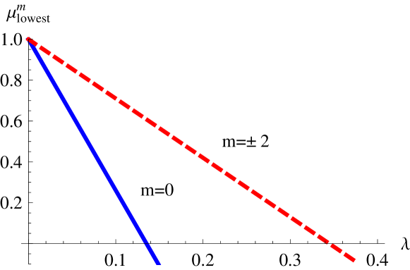
Figure 7: A plot of the lowest eigenvalues $\mu^{m}_{i}$ of $K_{ll^{\prime};m}^{3D}$ versus $\lambda$ for $m=0,\pm 2$. The instabilities of the $s$-channel (solid blue) and $d_{\pm 2}$-channel (dashed red) are revealed by the vanishing of their eigenvalues when $\lambda$ passes 0.135 and 0.35 respectively.

Compared to the compressibility calculation by the variational method in Ref. sogo2008 , in which it shows a stability condition equivalent to $\lambda\approx 0.42$. This is larger than our criterion $\lambda_{s}=0.135$ mentioned above. However, the calculation in Ref. sogo2008 did not take into account the Hartree contribution to the ground state energy. Although it is zero for rigorously homogeneous systems, it is actually singular due to the singularity of the Fourier transform of the 3D dipolar interaction $V_{3D}(\vec{q})$ as $\vec{q}\rightarrow 0$. Assuming an infinitesimal density wave vector $\vec{q}$ in the ground state, the Hartree self-energy contribution appears in $F_{00;0}(\vec{q})^{3D}$, and becomes most negative at $\theta_{q}=\frac{\pi}{2}$. In other words, Ref. sogo2008 sets $F^{3D}_{00;0}(\vec{q})=0$ which overestimates the stability of the 3D dipolar gas. Our result is supported by the numerical calculation given in Ref. ronen2009 , in which the Fermi surface instability manifests as the onset of an unstable collective mode at $\lambda_{s}\sim 0.14$. For the multi-component case, the critical value should be further suppressed by a factor of $1/N$ because DOS is $N$ times large, where $N$ is the number of components.

Similar static instability also occurs in the 2D dipolar system. Let us consider the specific case $\theta_{0}=\bar{\theta}_{0}$, which corresponds to the most anisotropic dipolar gas in 2D (Eq. 8). We numerically diagonalize the $K_{mm^{\prime}}^{2D}$ matrix in Eq. 84. The result shows that an instability would occur at $\lambda\sim 0.15$.

VI Collective excitations in the density and spin channels in 3D

In this section, we study the density-density response of the dipolar Fermi liquid and the corresponding collective excitations. The spin channel collective modes will also be studied in multi-component systems. Due to the anisotropic nature of the dipolar interaction, the response function exhibits anisotropic features. It shows the collective excitation of the zero sound which only propagates within a certain range of directions with anisotropic dispersion relations but become damped in other directions.

In the following, we will first present the generalized dynamical response of the dipolar system for 2 and 3D in Sect. VI.1, which is followed by the 3D collective excitations in Sect. VI.2. In order to obtain a clearer picture about the contribution of each mode towards the zero sound, we first consider the simplest $s$-wave channel in 3D only, where we will see how the zero sound propagation is restricted in certain propagation direction relative to the external electric field orientation. We then proceed to a more quantitative calculation by considering the correction from the $p$-channel. After that, we discuss the possible spin collective spin mode in Sect. VI.3.

VI.1 Generalized dynamical response functions

For the purpose to study collective modes, we define $\delta\nu_{\vec{p}}$ as the variation of Fermi distribution respect to the equilibrium Fermi surface with the dipolar interaction strength $\lambda$. Compared to the definition $\delta n_{\vec{p}}$ in Eq. 33 and $\delta n(\Omega_{k})$ in Eq. 71 which refer to the non-interacting Fermi surface, their spheric harmonic components are the same except $\delta\nu_{20}=\delta n_{20}-\delta n^{0}_{20}$ in the channel of $(l,m)=(2,0)$. $n^{0}_{20}$ refers to the equilibrium Fermi surface nematic distortion.

To start with, we consider the standard Boltzmann transport equation for the Fermi liquid baym1991 ; negele1988

$$\delta\nu_{\vec{p}}+\frac{\vec{v}_{\vec{p}}^{3D}\cdot\vec{q}}{\omega-\vec{v}_{\vec{p}}^{3D}\cdot\vec{q}}\frac{\partial n_{p}}{\partial\epsilon_{HF,p}}\int\frac{d^{3}p^{\prime}}{(2\pi)^{3}}f^{3D}(\vec{p},\vec{p}^{\prime})\delta\nu_{\vec{p}^{\prime}}=0.\ \ \$$ (88)

where $\vec{v}_{\vec{p}}^{3D}$ is the Fermi velocity in Eq. 25, $\epsilon_{HF,p}$ is the Hartree-Fock single particle spectrum and $f^{3D}(\vec{p},\vec{p}^{\prime})$ being the 3D Landau interaction in Eq. 35. This equation is equivalent to

$$\delta\nu(\Omega_{p})-\frac{N^{3D}(\Omega_{p})\vec{v}_{\vec{p}}\cdot\vec{q}}{\omega-\vec{v}_{\vec{p}}\cdot\vec{q}}\int\frac{d\Omega_{p^{\prime}}}{4\pi}f_{\vec{p}\vec{p}^{\prime}}\delta\vec{\nu}(\Omega_{p^{\prime}})=0.$$ (89)

After the spherical harmonic decomposition, we arrive at the generalized transport equation:

$$\sum_{l^{\prime}m^{\prime}}\Big{\{}\delta_{ll^{\prime}}\delta_{mm^{\prime}}+\sum_{l^{\prime\prime}}\chi_{ll^{\prime\prime};mm^{\prime}}^{3D}(\omega,\vec{q})F^{3D}_{l^{\prime\prime}l^{\prime};m^{\prime}}\Big{\}}\delta\nu_{l^{\prime}m^{\prime}}=0,\ \ \$$ (90)

where

$$\chi_{ll^{\prime};mm^{\prime}}^{3D}(\omega,\vec{q}) = -\frac{1}{\sqrt{(2l+1)(2l^{\prime}+1)}}\int d\Omega_{p}\frac{N^{3D}(\Omega_{\vec{p}})}{N^{3D}_{0}}$$ (91)

$$\times Y^{*}_{lm}(\Omega_{\vec{p}})\frac{\vec{v}_{p}^{3D}.\vec{q}}{\omega-\vec{v}_{p}^{3D}.\vec{q}}Y_{l^{\prime}m^{\prime}}(\Omega_{\vec{p}}),$$

where $F^{3D}_{ll^{\prime};m}$ is the Landau parameters defined in Eq. 39. Due to the dipolar anisotropy and the propagation direction of $\vec{q}$, $\delta\nu_{lm}$ in different channels are coupled. The dispersion of the collective modes can be obtained by equating the determinant of the above matrix equation to zero. The formalism above is not restricted to dipolar system and can by applied to any 3D Fermi liquid with azimuthal but not rotational symmetry.

Generally speaking, in order to calculate the zero sound propagation of these anisotropic systems, one has to deal with the above infinite matrix equation. However, in this 3D dipolar system, it turns out that the physics of zero sound is well captured by considering only the $s$ and longitudinal $p$ channels. In order to avoid complication, in the following, we start by examining the $s$-channel only, where the anisotropic feature of zero sound already appears in terms of a limited propagation direction and an anisotropic sound velocity. Afterwards, we consider the effect of the longitudinal $p$-wave mode, where a quantitative zero sound velocity is obtained as a function of propagation angle and this is in good agreement with a numerical study performed in Ref.ronen2009 .

VI.2 The 3D density channel collective mode: zero sound

VI.2.1 The $s$-wave channel

Let us warm up by only keeping the $s$-wave channel component in Eq. 91. To the lowest order of $\lambda$, we only keep the anisotropic Landau parameter of $F_{00;0}(\vec{q})$ which explicitly depends on the direction of $\vec{q}$, and completely neglect the anisotropic DOS and Fermi velocity. Thus the $\chi_{00;00}^{3D}(\omega,\vec{q})$ is simply the standard textbook result which reads at small values of $s=\omega/v_{f0}^{3D}q\ll 1$ as

$$\chi_{00;00}^{3D}(\vec{q},\omega)=N^{3D}_{0}\Big{\{}1-{s\over 2}\ln|{1+s\over{1-s}}|+i{\pi\over 2}s\Theta(s<1)\Big{\}}.$$

(92)

The collective excitation is determined by the pole of it:

$$1+F^{3D}_{00;0}(\Omega_{\vec{q}})\chi^{3D}_{00;00}=0.$$ (93)

$s>1$ is needed to ensure the collective mode underdamped.

Eq. 93 gives rise to an anisotropic zero sound velocities which explicitly depends on the propagation direction of $\theta_{q}$ as

$$\omega^{(0)}_{3D}(q,\theta_{q})=c_{3D}^{(0)}(\theta_{q})q,$$ (94)

where

$$\frac{c_{3D}^{(0)}(\theta_{q})}{v_{f0}^{3D}}=\left\{\begin{array}[]{rr}1+2e^{-\frac{1}{4\pi\lambda P_{2}(\cos\theta_{q})}};&\mbox{ $8\pi\lambda P_{2}(\cos\theta_{q})\ll 1$}\\ \sqrt{\frac{8\pi}{3}\lambda P_{2}(\cos\theta_{q})};&\mbox{$8\pi\lambda P_{2}(\cos\theta_{q})\gg 1$}\end{array}\right.$$ (97)

(98)

for $\theta_{q}<\bar{\theta}_{0}$ or $\theta_{q}>\pi-\bar{\theta}_{0}$, where $\bar{\theta}_{0}$ is defined in Eq. 2. The zero sound is well-defined around the north and south poles of the Fermi surface, where the interaction is most repulsive. On the other hand, for $\bar{\theta}_{0}<\theta_{q}<\pi-\bar{\theta}_{0}$, $F_{00;0}(\Omega_{q})$ becomes negative, the solution shows $s<1$ which means the dispersion goes into the particle-hone continuum and ceases to be a sharp collective mode.

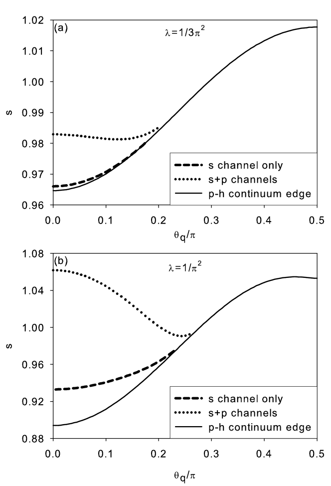
Figure 8: Dispersions of the zero sound $s(\theta_{q})=\omega(\theta_{q})/v_{f0}^{3D}q$ for the pure dipolar interaction including the coupling between the $s$-wave and the longitudinal $p$-wave modes for $\lambda=\frac{1}{3\pi^{2}},\frac{1}{\pi^{2}}$. The $s$-wave approximation is included for comparison which is valid in the limit of a large component number $N$ with the replacement of $\lambda\rightarrow N\lambda$. When the sound speed hits the particle hole continuum, the sound becomes damped. These results are in good agreement with a numerical study in Ref. ronen2009 . (The parameters are chosen for a better comparison with the Ref. ronen2009 , where their parameters $D=3\pi^{2}\lambda$ are chosen to be 1 and 3.)

In order to refine the above calculation, one has to take into account the anisotropic Hartree-Fock single particle spectra and thus the anisotropic Fermi surface. In this sense, the full $\chi^{3D}_{00;00}(\omega,\vec{q})$ function is given by

$$\chi_{00;00}^{3D}(\omega,\vec{q}) = -\int\frac{d\Omega_{p}}{4\pi N^{3D}_{0}}\frac{N^{3D}(\Omega_{p})(\vec{q}\cdot\nabla_{p}\epsilon_{HF}(\vec{p}))}{\omega-\vec{q}\cdot\nabla_{p}\epsilon_{HF}(\vec{p})+i\eta}$$

$$= 1-\int\frac{d\Omega_{p}}{4\pi}\frac{N^{3D}(\Omega_{p})}{N^{3D}_{0}}\frac{s}{s-f(\Omega_{p},\Omega_{q})+i\eta},$$

where $N^{3D}(\Omega_{p})=N_{0}[1+\frac{5\pi}{3}P_{2}(\cos\theta_{p})]$ defined in Eq. 30 and $\epsilon_{HF}(\vec{k})$ is the Hartree-Fock single particle spectra. The angular form factor $f(\Omega_{p},\Omega_{q})$ is defined as

$$f(\Omega_{p},\Omega_{q}) = \frac{\vec{q}\cdot\nabla_{p}\epsilon_{HF}(\vec{p})}{v_{f0}^{3D}q}=[1-\frac{\pi}{3}\lambda P_{2}(\cos\theta_{p})]$$ (100)

$$\times \big{[}\sin\theta_{q}\sin\theta_{p}\cos\phi_{p}+\cos\theta_{q}\cos\theta_{p}\big{]}$$

$$+ \lambda\pi\sin 2\theta_{p}(\sin\theta_{q}\cos\theta_{p}\cos\phi_{p}$$

$$- \cos\theta_{q}\sin\theta_{p}),$$

where the propagation direction $\vec{q}$ is chosen in the $xz$-plane with the polar angle $\theta_{q}$. Eq. 93 is solved numerically and plotted in Fig. 8 along with the edge of particle-hole continuum and the further refined result including the $p$-wave channel correction. (We postpone the discussion of it until we include the $p$-channel correction in the following subsection.)

So far, we neglect the coupling between the $s$-wave and other high partial channel Fermi surface excitations. This approximation is valid if the Landau matrix elements in other channels are small compared to that in the $s$-wave channel. This is justified in the multi-component case with a large $N$ in which $F_{00;0}$ has a large $N$-enhancement compared to all of other matrix elements. Thus the result of Eq. 98 is correct in the large $N$-limit with the replacement of $\lambda$ by $N\lambda$. However, for the single component dipolar interaction, i.e., $N=1$, the zero sound dispersion is modified from the coupling to the longitudinal $p$-wave channel modes as explained below.

VI.2.2 The correction from the coupling to the longitudinal $p$-wave channel

The coupling between the $s$-wave and other high partial wave channel Fermi surface excitations, say, the $p$-wave longitudinal excitation, can significantly change the zero sound dispersion. This effect is particularly important if the Landau interaction in the $F_{1}$-channel is not small compared to $F_{0}$. For example, the zero sound velocity is measured as $s=3.6\pm 0.01$ in ³He at 0.28 atm, while $F_{0}^{s}=10.8$ only gives $s=2$. The inclusion of the coupling to the $p$-wave channel $F_{1}^{s}=6.3$ gives rise to the accurate value of $s=3.6$ negele1988 . Below we consider this coupling for the single component dipolar Fermi gas.

Now, we consider the coupling between the $s$-wave and the longitudinal $p$-wave channel modes in our 3D dipolar system. The formalism developed in Subsect. VI.1 have 3 $p$-wave modes; $l=1$ and $m=0,\pm 1$, which mixes the longitudinal and transverse modes. It turns out that it is better to reformulate the generalized response function by putting the spherical harmonic expansion $Y_{lm}$ relative to the $\vec{q}$ direction. Due to the explicit anisotropy, the longitudinal and transverse $p$-wave components should be mixed. Nevertheless, the transverse $p$-wave channel mode is overdamped for small positive value of Landau parameters, thus they do not affect the zero sound much. We only keep the mixing between $s$-wave and the longitudinal $p$-wave modes.

The corresponding transport equation becomes a $2\times 2$ matrix equation and the collective mode can be solved from:

$$\mbox{Det}[1+N(\vec{q},\omega)]=0,$$ (101)

where the matrix kernel of $N(\vec{q},\omega)$ reads

$$N(\vec{q},\omega)=\left(\begin{array}[]{cc}\chi_{00;00}^{3D}(\vec{q},\omega)F_{00;0}^{3D}(\vec{q})&\tilde{\chi}_{10;00}^{3D}(\vec{q},\omega)\frac{\tilde{F}_{110}^{3D}(\vec{q})}{3}\\ \tilde{\chi}_{10;00}^{3D}(\vec{q},\omega)F_{00;0}^{3D}(\vec{q})&\tilde{\chi}_{11;00}^{3D}(\vec{q},\omega)\frac{\tilde{F}_{11;0}^{3D}(\vec{q})}{3}\end{array}\right).$$ (104)

$\tilde{F}_{11;0}^{3D}(\vec{q})$ is the longitudinal $p$-wave Landau parameter defined as

$$\tilde{F}_{11;0}^{3D}(\vec{q}) = N^{3D}_{0}\int d\Omega_{p}d\Omega_{p}^{\prime}f^{3D}(\vec{p}_{F},\vec{p}_{f}^{\prime})(\hat{q}.\hat{p})^{2}$$ (106)

$$= \cos^{2}\theta_{q}F_{11;m=0}^{3D}+\sin^{2}\theta_{q}F_{11;m=\mp 1}^{3D}$$

$$= F_{11,m=0}^{3D}P_{2}(\cos\theta_{q})=\frac{18\pi}{5}P_{2}(\cos\theta_{q}).\ \ \$$

The relevant response functions are correspondingly modified as:

$$\tilde{\chi}^{3D}_{10;00}(\vec{q},\omega) = -\sqrt{3}\int\frac{d\Omega_{p}}{4\pi}\frac{N^{3D}(\Omega_{p})}{N^{3D}_{0}}\frac{(\hat{q}\cdot\hat{p})f(\Omega_{p},\Omega_{q})}{s-f(\Omega_{p},\Omega_{q})}$$

$$\tilde{\chi}^{3D}_{11;00}(\vec{q},\omega) = -3\int\frac{d\Omega_{p}}{4\pi}\frac{N^{3D}(\Omega_{p})}{N^{3D}_{0}}\frac{(\hat{q}\cdot\hat{p})^{2}f(\Omega_{p},\Omega_{q})}{s-f(\Omega_{p},\Omega_{q})}$$

where $\vec{q}$ lies in the $xz$-plane with the polar angle $\theta_{q}$, and $\hat{q}\cdot\hat{k}=\sin\theta_{q}\sin\theta_{k}\cos\phi_{k}+\cos\theta_{q}\cos\theta_{k}$.

Before we solve Eq. 101, we can get a qualitative picture by approximating the Fermi surface and density of state to be spherical first. Under this approximation, in the long wavelength limit $\vec{q}\rightarrow 0$, Eq. 101 can be analytically simplified to:

$$\frac{-1}{F_{00;0}^{3D}(\vec{q})+\frac{s^{2}\tilde{F}_{11;0}^{3D}(\vec{q})}{1+\frac{\tilde{F}_{11;0}^{3D}(\vec{q})}{3}}}=1-\frac{s}{2}\ln|\frac{1+s}{1-s}|,$$ (108)

which resembles the usual zero sound condition by considering only $F_{0}$ and $F_{1}$ parameters in an ordinary isotropic Fermi liquid negele1988 . The difference is that the Landau parameters now have an explicit $\vec{q}$ dependence. Because $F_{00;0}(\vec{q})$ and $F_{11;0}(\vec{q})$ have the same angular dependence, including the longitudinal $p$-wave channel mode does not change the propagation angular regime, but enhance the zero sound velocity.

Now, we solve Eq. 101 numerically by taking into account the anisotropic fermion spectra and Fermi surface. The zero sound propagation as a function of $\theta_{q}$ is plotted in Fig. 8. The calculation that only involve the $s$-channel is also included for comparison. There are two features: a restricted zero sound propagation angle and an anisotropic propagation velocity, $s$. The first feature is due to the fact that the sound enters the particle-hole continuum for large $\theta_{q}$ and is thus damped. It is clear that, in terms of the critical angle where zero sound terminate, the $s$-wave approximation is qualitatively justified. However, when we consider the zero sound speed as a function of $\theta_{q}$, the longitudinal $p$-wave mode modifies it considerably. These results are in a good agreement with a fully numerical calculation based on the same Boltzmann transport theory ronen2009 . This indicates that the physics of collective excitation of the 3D dipolar system is well captured by considering only the $s$ and longitudinal $p$-channels.

The zero sound velocity is affected by both the value of Landau parameters and the Fermi velocity as shown in Eq. 98. For the relatively large value of $\lambda=\frac{1}{\pi^{2}}$, the Landau parameters play a more important role. Thus the sound velocity is largest for $\vec{q}$ along the north and south poles where $F_{00;0}^{3D}(\vec{q})$ and $F_{11;0}^{3D}(\vec{q})$ are largest. As the propagation deviates from them, the sound velocity first becomes softened. As the velocity hits the upper edge of the particle-hole continuum, the zero sound ceases to propagate. At a small value of $\lambda=\frac{1}{3\pi^{2}}$, Fig. 8 shows the upturn of zero sound velocity before it hits the particle-hole continuum, which is largely determined by the anisotropic Fermi velocity. We also plot the eigenvector for the zero sound mode for the solution of Eq. 101. The $s$ and the longitudinal $p$-wave components are comparable to each other.

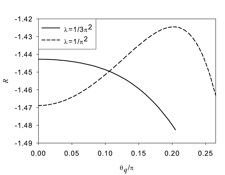
Figure 9: The ratio between the longitudinal $p$-wave and the $s$ components in the eigenvectors of the 3D zero sound, i.e. $R=\delta\nu_{10;0}/\delta\nu_{00;0}$, for $\lambda=\frac{1}{3\pi^{2}}$ and $\frac{1}{\pi^{2}}$.

VI.3 3D Collective spin mode in the longitudinal $p$-wave channel

In addition to the zero sound mode, collective excitations may also exist in the spin channel. Because $F^{3D,a}_{00;0}=0$ (see definition in Eq. 50), there is no well-defined $s$-wave channel spin excitations. Nevertheless, the longitudinal $p$-wave channel mode becomes a propagating mode. The formalism to determine its dispersion is very similar to Eq. 90 by replacing $F^{s}_{ll^{\prime};m}$ to $F^{a}_{ll^{\prime};m}$. Only keeping the longitudinal $p$-wave channel, we have

$$1+\tilde{F}^{3D,a}_{11;0}(\vec{q})\tilde{\chi}_{11;00}^{3D}(\vec{q},\omega)=0.$$ (109)

$\tilde{F}^{3D,a}_{11;0}(\vec{q})=F^{a}_{11;0}P_{2}(\cos\theta_{q})$ which is the same as $\tilde{F}^{3D,s}_{11;0}(\vec{q})$ at the Hartree-Fock level, and $\tilde{\chi}^{3D}_{11;00}$ is also the same as in Eq. LABEL:eq:bubble_2. The dispersion for this $p$-wave longitudinal spin collective mode is plotted in Fig. 10 for $\lambda=\frac{1}{\pi^{2}}$. Again, we have an anisotropic sound velocity subject to a finite propagation regime, where the excitation is damped when its dispersion enters the particle-hole continuum.

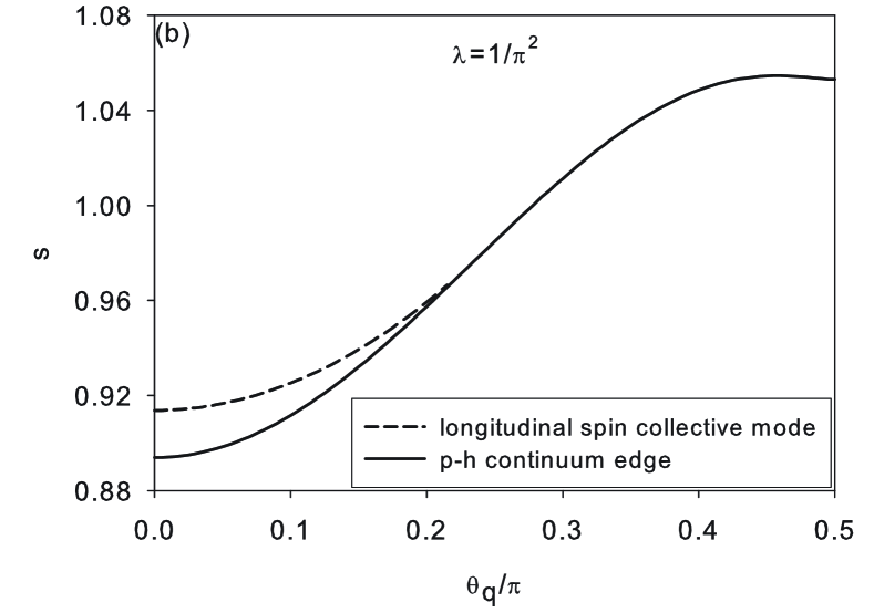
Figure 10: 3D collective spin mode in the longitudinal $p$-channel for $\lambda=\frac{1}{\pi^{2}}$. The sound speed continuously decreases as $\theta_{q}$ increases and terminates at certain critical angle.

In $N$-component dipolar gases with the $SU(N)$ symmetry, there are $N^{2}-1$ branches of longitudinal $p$-wave spin model. They are essentially the fluctuating longitudinal spin current mode. The is a novel collective mode which has not been observed in condensed matter systems before.

VII Conclusions and Outlook

In summary, we studied the anisotropic Fermi liquid states of the cold atomic dipolar Fermi gases which possesses many exotic features. The feature of the $d_{z^{2}-3r^{2}}$ symmetry of the 3D dipolar interaction and the $d_{x^{2}-y^{2}}$ symmetry of the 2D dipolar interaction nicely render most analytic calculations possible. The same anisotropy exhibits at the leading order of perturbation theory in many ways such as the Fermi surface anisotropy, Fermi velocity and effective masses. The Landau parameters in isotropic Fermi liquid states are generalized to the Landau interaction matrix which has the tri-diagonal structure as a result of the Wigner-Eckart theory. Physical susceptibilities receive renormalization from the Landau interaction matrix. With large dipolar interactions, dipolar Fermi surfaces become collapse along the directions perpendicular to the dipolar orientation. We also studied the collective mode in the density and spin channels. The zero sound exhibits anisotropic dispersion relation with largest propagation velocity along polar direction. The $p$-wave longitudinal spin channel mode is a well defined propagating mode for any propagation directions.

So far, we have only considered the spatial homogeneous systems. However, the realistic experimental systems have confining traps, which should bring corrections to properties discussed above as studied in Refs sogo2008 ; miyakawa2008 ; tian2008 . In the case of soft confining trap potentials, we can treat the inhomogeneity by using the local density approximation. Around each position $\vec{r}$, we can define a local Fermi energy and the local Fermi surface which are determined by the local molecule density. The molecule density is the highest at the center of the trap, thus both the absolute interaction energy scale and the dimensionless interaction strength are strongest at the center. Thus the thermodynamic instabilities are strongest at the center of the trap and become weaker as moving towards the edge. For the collective excitation of zero sound, the local sound velocity is largest in the center. As a result, the local propagation wavevector increases from the center to the edge to maintain the excitation eigen-frequency the same in the entire trap. The collective modes have more server damping in the edge area because the molecule density is low and thus is less quantum degenerate than the center. A detailed study of all the above effects will be presented in a later publication.

Other open questions to be studied in the future include the issues of higher-order (i.e. beyond Hartree-Fock theory) interaction corrections and finite temperature corrections. The theory developed in this work is strictly valid for weak interaction and low temperatures. For example, an important aspect of the dipolar Fermi gas is the finite life time and the Fermi liquid wavefunction renormalization factor $Z$ of quasiparticles. Both of them naturally also develop anisotropies due to the dipolar interaction. However, they begin to appear at the level of the second order perturbation theory beyond the Hartree-Fock level, thus their anisotropies should be of an even higher order spheric harmonics than the $d$-wave. Another issue is the screening effect in the dipolar Fermi gases which may change its long range negative in 3D. These effects will be deferred to another paper chan2009a .

- (1) A. J. Leggett, Rev. Mod. Phys. 47, 331 (1975).
- (2) G. Baym and C. Pethick, Landau Fermi-liquid theory (John Wiley & Sons, Inc., ADDRESS, 1984).
- (3) I. I. Pomeranchuk, Soviet Physics Jetp-Ussr 8, 361 (1959).
- (4) V. Oganesyan, S. A. Kivelson, and E. Fradkin, Phys. Rev. B 64, 195109 (2001).
- (5) C. J. Halboth and W. Metzner, Phys. Rev. Lett. 85, 5162 (2000).
- (6) J. Nilsson and A. H. Castro Neto, Phys. Rev. B 72, 195104 (2005).
- (7) H. Y. Kee, Phys. Rev. B 67, 73105 (2003).
- (8) C. Wu and S. C. Zhang, Phys. Rev. Lett. 93, 36403 (2004).
- (9) C. Wu, K. Sun, E. Fradkin, and S.-C. Zhang, Phys. Rev. B 75, 115103 (2007).
- (10) C. M. Varma, Philos. Mag. 85, 1657 (2005).
- (11) J. E. Hirsch, Phys. Rev. B 41, 6820 (1990).
- (12) W. Kohn and J. M. Luttinger, Phys. Rev. Lett. 15, 524 (1965).
- (13) S. Ospelkaus, K. K. Ni, M. H. G. de Miranda, B. Neyenhuis, D. Wang, S. Kotochigova, P. S. Julienne, D. S. Jin, and J. Ye, arXiv.org:0811.4618, 2008.
- (14) K. K. Ni, S. Ospelkaus, M. H. G. de Miranda, A. Pe’er, B. Neyenhuis, J. J. Zirbel, S. Kotochigova, P. S. Julienne, D. S. Jin, and J. Ye, Science 322, 231 (2008).
- (15) A. Griesmaier, J. Werner, S. Hensler, J. Stuhler, and T. Pfau, Phys. Rev. Lett. 94, 160401 (2005).
- (16) J. J. McClelland and J. L. Hanssen, Phys. Rev. Lett. 96, 143005 (2006).
- (17) M. Lu, S. H. Youn, and B. L. Lev, arXiv.org:0912.0050, 2009.
- (18) T. Koch, T. Lahaye, J. Metz, B. Frohlich, A. Griesmaier, and T. Pfau, Nature Physics 4, 218 (2008).
- (19) T. Lahaye, C. Menotti, L. Santos, M. Lewenstein, and T. Pfau, Rep. Prog. Phys. 72, 126401 (2009).
- (20) T. Lahaye, J. Metz, T. Koch, B. Frohlich, A. Griesmaier, and T. Pfau, arXiv.org:0808.3876, 2009.
- (21) C. Menotti, M. Lewenstein, T. Lahaye, and T. Pfau, arXiv.org:0711.3422, 2007.
- (22) T. Sogo, L. He, T. Miyakawa, S. Yi, H. Lu, and H. Pu, New J. Phys. 11, 055017 (2008).
- (23) T. Miyakawa, T. Sogo, and H. Pu, Phys. Rev. A 77, 061603 (2008).
- (24) Chi-Ming Chang, Wei-Chao Shen, Chen-Yen Lai, Pochung Chen, Daw-Wei Wang, Phys. Rev. A 79, 053630 (2009).
- (25) M. A. Baranov, M. S. Mar’enko, V. S. Rychkov, and G. V. Shlyapnikov, Phys. Rev. A 66, 013606 (2002).
- (26) M. A. Baranov, Ł. Dobrek, and M. Lewenstein, Phys. Rev. Lett. 92, 250403 (2004).
- (27) M. A. Baranov, Physics Reports 464, 71 (2008).
- (28) M. A. Baranov, H. Fehrmann, and M. Lewenstein, Phys. Rev. Lett. 100, 200402 (2008).
- (29) G. M. Bruun, E. Taylor, Phys. Rev. Lett. 101, 245301 (2008).
- (30) B. M. Fregoso, K. Sun, E. Fradkin, and B. L. Lev, New J. Phys. 11, 103003 (2009).
- (31) B. M. Fregoso and E. Fradkin, Phys. Rev. Lett. 103, 205301 (2009).
- (32) C. Wu, J. P. Hu, and S. C. Zhang, Phys. Rev. Lett. 91, 186402 (2003).
- (33) C. Wu, Mod. Phys. Lett. B 20, 1707 (2006).
- (34) L. D. Landau, Sov. Phys. JETP 3, 920 (1957).
- (35) L. D. Landau, Sov. Phys. JETP 8, 70 (1959).
- (36) S. Ronen and J. Bohn, arXiv.org:0906.3753, 2009.
- (37) W. Negele and H. Orland, Quantum many-particle systems (Perseus Books (Sd), ADDRESS, 1988).
- (38) Y. Y. Tian and D. W. Wang, arXiv:0808.1342.
- (39) C. K. Chan, W. C. Lee, C. Wu, and D. Das Sarma, in preparation.