Dynamical Models of Terrestrial Planet Formation

Jonathan I. Lunine^∗, Lunar and Planetary Laboratory, The University of Arizona, Tucson AZ USA, 85721. jlunine@lpl.arizona.edu

David P. O’Brien, Planetary Science Institute, Tucson AZ USA 85719

Sean N. Raymond, Center for Astrophysics and Space Astronomy, UCB 389, University of Colorado, Boulder, CO 80309-0389 and Laboratoire d’Astrophysique de Bordeaux (CNRS; Universit Bordeaux I), BP 89, F-33270 Floirac, France

Alessandro Morbidelli, Obs. de la Côte d’Azur, Nice, F-06304 France

Thomas Quinn, Department of Astronomy, University of Washington, Seattle USA 98195

Amara L. Graps, Southwest Research Institute, Boulder CO USA 80302

Accepted for publication in Advanced Science Letters June 10, 2009

^∗Corresponding author

Abstract

We review the problem of the formation of terrestrial planets, with particular emphasis on the interaction of dynamical and geochemical models. The lifetime of gas around stars in the process of formation is limited to a few million years based on astronomical observations, while isotopic dating of meteorites and the Earth-Moon system suggest that perhaps 50-100 million years were required for the assembly of the Earth. Therefore, much of the growth of the terrestrial planets in our own system is presumed to have taken place under largely gas-free conditions, and the physics of terrestrial planet formation is dominated by gravitational interactions and collisions. The earliest phase of terrestrial-planet formation involve the growth of km-sized or larger planetesimals from dust grains, followed by the accumulations of these planetesimals into $\sim$100 lunar- to Mars-mass bodies that are initially gravitationally isolated from one-another in a swarm of smaller planetesimals, but eventually grow to the point of significantly perturbing one-another. The mutual perturbations between the embryos, combined with gravitational stirring by Jupiter, lead to orbital crossings and collisions that drive the growth to Earth-sized planets on a timescale of $10^{7}-10^{8}$ years. Numerical treatment of this process has focussed on the use of symplectic integrators which can rapidy integrate the thousands of gravitationally-interacting bodies necessary to accurately model planetary growth. While the general nature of the terrestrial planets–their sizes and orbital parameters–seem to be broadly reproduced by the models, there are still some outstanding dynamical issues. One of these is the presence of an embryo-sized body, Mars, in our system in place of the more massive objects that simulations tend to yield. Another is the effect such impacts have on the geochemistry of the growing planets; re-equilibration of isotopic ratios of major elements during giant impacts (for example) must be considered in comparing the predicted compositions of the terrestrial planets with the geochemical data. As the dynamical models become successful in reproducing the essential aspects of our own terrestrial planet system, their utility in predicting the distribution of terrestrial planet systems around other stars, and interpreting observations of such systems, will increase.

Keywords: planets, dynamics, formation, Earth, water, Moon

Dedicated to George Wetherill (1925-2006), pioneer in studies of the formation of the terrestrial planets.

1 Introduction

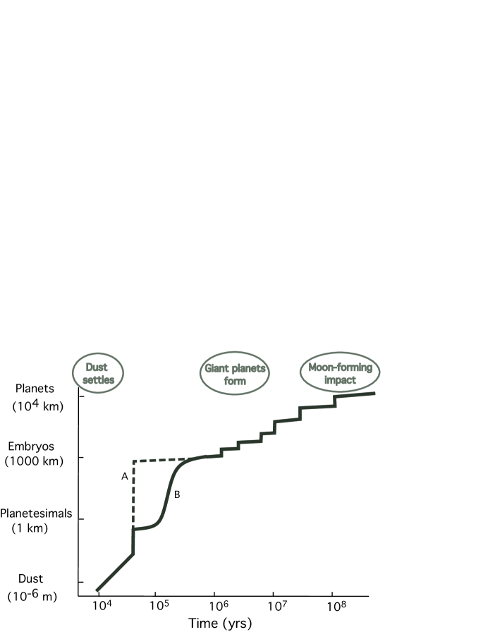
Figure 1: An illustration of the stages of terrestrial planet growth and the relevant timescales not to scale; image from ¹⁴⁴. See §3 for details.

The formation of the terrestrial planets remains one of the enduring problems in planetary science and (in view of the expectation of large numbers of extrasolar terrestrial-type planets) astrophysics today. The complexity of terrestrial geochemistry, constraints on timescales, the presence of abundant water on the Earth, and the curious geochemical and dynamical relationships between the Earth and the Moon are among the problems that must be addressed by models. Pioneering studies by Safronov ¹ and successors such as Weidenschilling ² established the basic physics of gas-free accretion. The effects of gas on accretion were examined somewhat later, most notably by the “Kyoto” school of Hayashi and collaborators ³. In the 1980’s, studies of terrestrial planet formation advanced further thanks to George Wetherill ⁴, his students and postdoctoral collaborators, who highlighted the basic problems of obtaining the correct low planetary eccentricities and inclinations, as well as producing a diversity of sizes ranging from Earth through Mars and Mercury. Breakthroughs in the subject came through the development of special numerical approaches to the problem, as well as theoretical insights that allowed for the right starting boundary conditions. Additional geochemical considerations, including formation timescales derived from radioactive isotopic ratios, and stable isotopic constraints on source regions, continue to challenge the models today. Decades of research have established a rough timeline of events during the formation of the Solar System’s terrestrial planets. These are summarized in Figure 1, which shows the many steps which occurred during the formation of the Earth.

The classical view, developed in the 1960’s and 1970’s, is that the planetesimals grow gradually, from collisional coagulation of pebbles and boulders. The growth becomes exponential (runaway) when the first massive bodies appear in the disk ⁵, ⁶. However, it is not clear how ordered growth can procede beyond 1 meter in size, the so-called meter-size barrier that we explain more extensively in section 2. A new view to by-pass the meter-size barrier is that boulders, pebbels and even chondrule-size particles can be concentrated in localized structures of a turbulent disk, where they form self-gravitating clumps. The size-equivalent of these clumps can be 10km ⁷, 100km ⁸ or 1,000 km ⁹, depending on the models and the physics that is accounted for. The growth rate of $\sim$ Moon-sized embryos decreases during oligarchic growth because of viscous stirring of planetesimals by the embryos and decreased gravitational focusing ¹⁰, ¹¹. Late-stage accretion begins when embryo-embryo collisions occur ¹², ¹³, and takes place in the presence of Jupiter and Saturn, which must have formed in less than $\sim$ 5 Myr ¹⁴. Late-stage accretion lasted for about 100 Myr in the Solar System based on radioisotopic chronometers. ¹⁵.

In this review we describe the numerical tools and theoretical concepts used in simulating terrestrial planet formation, and the geochemical constraints. We focus on two applications: (1) the origin of water on the Earth and (2) the predicted diversity of terrestrial planet systems around other stars. We begin by describing the astrophysical and geochemical constraints on timescales. We then describe the phases of planetesimal growth and the subsequent oligarchic growth of planetary embryos that set the boundary conditions for terrestrial planet formation, following which the numerical approach widely used today is outlined. We discuss results from the various groups that have conducted simulations, and how well certain constraints from observations are reproduced. The relevance of the formation of the Moon by giant impact in understanding terrestrial planet formation is considered. We then highlight application of the simulations to the origin of water on the Earth, and to simulation of extrasolar planetary systems. We close with a list of outstanding issues, and the possible directions for their solution.

2 Early Phases of Terrestrial Planet Formation

2.1 Planetesimal Formation

Planets form from disks created when clumps of interstellar gas and dust, organized in dense molecular clouds, collapse to form stars ¹⁶. The angular momentum content of typical clumps ensures that a portion of the collapsing material ends up in a disk, through which much of the mass works its way inward to the growing “protostar” and angular momentum continues to reside in the disk–fully consistent with the mass and angular momentum distribution of the Sun and planets. Disks undergo evolution from gas-dominated systems to “debris” disks in which only solids remain; based on astronomical observations most of the gas is gone within 6 million years after the collapse begins ¹⁷. (The appearance of the first solids in our solar system is reliably dated by meteorites to be 4.568 billion years ago ¹⁸).

“Planetesimal” is the term used to connote the fundamental building blocks of the planets whose growth is dominated by gravity rather than gas-drag. They are generally defined to be the smallest rocky bodies that are decoupled from the gaseous disk. The most commonly-assumed planetesimal size is 1 km, corresponding to a mass on the order of 10¹⁶ grams. However, km-sized bodies are not completely decoupled from the gas, in that their orbits are significantly altered by gas drag via relatively rapid ($\sim 10^{3}-10^{4}$ yr) damping of their eccentricities and inclinations, and much slower ($\sim 10^{6}$ yr) decay of their semimajor axes ¹⁹. In fact, the actual size distribution of bodies during the phase of gravity-dominated growth is determined by the formation mechanism of these bodies, which remains uncertain (see below). The planetesimal size is therefore used as a parameter in some models of later stages of planetary growth ²⁰.

Modeling planetesimal growth requires a detailed treatment of the structure of the gaseous disk, including turbulence, local pressure gradients, magnetic processes, and vortices. Models can be constrained by observations of dust populations in disks around young stars, although interpretation of observations remains difficult ²¹. There currently exist two qualitatively-different theories for planetesimal formation: collisional growth from smaller bodies eg., ²² and local gravitational instability of smaller bodies ⁷, ²³, ⁹, ⁸.

Collisional growth of micron-sized grains, especially if they are arranged into fluffy aggregates, appears efficient for relatively small particle sizes and impact speeds of $\sim 1\,m\,s^{-1}$ or slower²⁴, ²⁵, ²⁶; see the review by Dominik et al.(2007)²⁷. However, there is a constant battle between disk turbulence, which increases random velocities, and drag-induced settling, which reduces them ²⁸, ²⁹. Growth of particles in such collisions appears effective until they reach roughly 1 cm to 1 m in size. At that point, continued growth may be suppressed by collision velocities of $\geq 10\,m\,s^{-1}$ ³⁰, ²¹.

Meter-sized bodies are the barrier of planetesimal formation. As an object in the gaseous disk grows, it becomes less strongly-coupled to the gas such that its orbital velocity transitions between the gas velocity, which is slowed by partial pressure support, and the local Keplerian velocity. This increases the relative velocity between the object and the local gas such that the object feels a head wind which acts to decrease its orbital energy and cause the body to spiral toward the star. Large ($\geq$ 10s to 100s of meters) objects have enough inertia that orbital decay occurs slowly, but there exists a critical size for which orbital decay is fastest. For the case of rocky bodies in a gaseous disk, this critical size is roughly 1 m, and the timescale for infall for meter-sized bodies can be as short as 100 years. This is referred to as the ‘meter-size “catastrophe” or sometimes “barrier”, because the infall timescale is far shorter than typical growth timescales ³¹. Collisional growth models must therefore quickly cross the barrier at meter-sizes if they are to reach planetesimal sizes ²², ²⁶, ³².

The gravitational instability model for planetesimal formation suggests that a large number of small patches of particles could become locally gravitationally unstable and form planetesimals ¹, ⁷, ²³. (The criterion for gravitational instability of Keplerian disks appears already in Safranov (1960)) ³³. This process requires a concentration of meter-sized or smaller particles. If the density of solids in a small patch exceeds a critical value, then local gravitational instability can occur, leading to top-down formation of planetesimals. A concentration of small particles great by a large factor compared with the gas is the key to the process.

Models for the concentration of small particles often rely on structure within the gaseous component of the disk, generated by turbulence or self-gravity ³⁴, ³⁵. If the disk is even weakly turbulent, a size-dependent concentration of small particles can occur ³⁶, ³⁴, ²⁹. Pre-existant chondrule-sized particles may have been concentrated at these scales by such a mechanism, thus appearing as the basic building blocks of larger structures such as chondritic parent bodies.

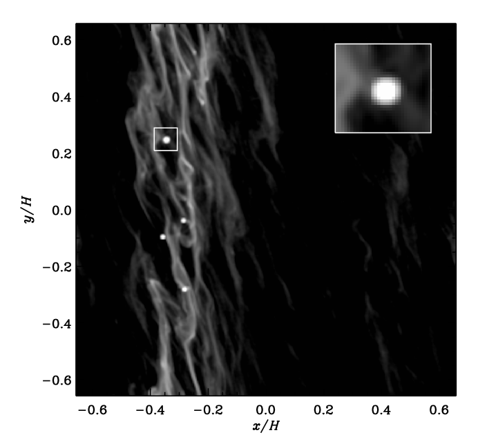
Figure 2: Concentration of boulder-sized particles in MRI-turbulent structures in the model of Johansen et al. (2007) Johansen2007 ⁹. The x and y axes are shown in units of the disk’s vertical scale height H, and this snapshot is from seven orbital times after a clumping event occurred. The greyscale represents the local density of particles, and the solid circles show the location of four clumps that are each more massive than Ceres (i.e., they correspond to $\sim$ 1000 km or larger “planetesimals” (or small embryos) in the overdense filament. The inset focuses on one clump as shown. Original figure provided by Anders Johansen.

Self-gravitating clumps of chondrules may end up as 10- to 100-km sized planetesimals; in this case particles don’t collapse rapidly on the dynamical timescale but slowly contract into planetesimals ⁸. Turbulence can also concentrate larger, meter-sized particles by producing local pressure maxima which can act as gathering points for small bodies. As for the meter-size catastrophe, boulder-sized objects are the fastest to drift toward pressure maxima ³⁷, ³⁸. The concentration in these regions can be further increased via a streaming instability between the gas and solids ³⁹, ⁴⁰, and gravitational collapse of the clumps can occur in these dense regions. Johansen et al.Johansen2007 ⁹ showed that planetesimals can form via this process and that the particle clumps (i.e., the rubble-pile planetesimals) have a distribution of sizes that ranges up to 1000 km or larger. Figure 2 shows the surface density of boulder-sized particles in a disk in which four 1000 km-scale objects have formed ⁹. An alternate location for planetesimal formation via gravitational instability are regions with an increased local density of solids ⁴¹. Other ways to concentrate solids include drag-induced in-spiralling to disk edges (²³, vortices ⁴², ⁴³, or photo-evaporative depletion of the gas layer ⁴⁴.

2.2 Oligarchic growth

Relative velocities in the disk temd to remain low, whether because of damping of eccentricities by gas drag ¹⁹, collisional damping, or merely the presence of a few larger bodies that can limit the dispersion velocities of the smaller ones. Bodies that are slightly larger than the typical size can increase their collisional cross sections due to gravitational focusing and thereby accelerate their growth ¹, ⁵:

$$\frac{dM}{dt}=\frac{\pi R^{2}\Sigma\,v_{rand}}{2\,H}F_{g}(v_{rand}),$$ (1)

where $R$ represents the body’s physical radius, $v_{rand}$ represents the velocity dispersion of planetesimals, $\Sigma$ is the local surface density of planetesimals, $H$ is the scale height of the planetesimal disk, and $F_{g}$ is the so-called gravitational focussing factor, which depends on $V_{rand}$. The expression for $F_{g}$ is complicated ⁴⁵, ⁴⁶; for moderate $v_{rand}$, it can be approximated by $\left(1+\frac{v_{esc}2}{v_{rand}2}\right)$, where $v_{esc}$ is the escape speed from the body’s surface.

While random velocities are small, gravitational focusing can increase the growth rates of bodies by a factor of hundreds, such that $dM/dt\sim M^{4/3}$, leading to a phase of rapid “runaway growth” ⁴⁷, ⁵, ⁶, ⁴⁸, ¹⁰, ¹¹, ⁴⁹, ⁵⁰. The length of this phase depends on the timescale for $v_{rand}$ to increase, which depends on a combination of eccentricity growth via interactions with large bodies and eccentricity damping. For small ($\sim$100 m-sized) planetesimals, gas drag is stronger such that runaway growth can be prolonged and embryos may be larger and grow faster ⁵¹, ²⁰.

As large bodies undergo runaway growth, they gravitationally perturb nearby planetesimals. The random velocities of planetesimals are therefore increased by the larger bodies in a process called “viscous stirring” ¹⁰. During this time, the random velocities of large bodies are kept small via dynamical friction with the swarm of small bodies ¹¹. As random velocities of planetesimals increase, gravitational focusing is reduced, and the growth of large bodies is slowed to the geometrical accretion limit, such that $dM/dt\sim M^{2/3}$ (⁵², ⁵¹). Nonetheless, large bodies continue to grow, and jostle each other such that a characteristic spacing of several mutual Hill radii $R_{H,m}$ is maintained ($R_{H,m}\equiv 0.5[a_{1}+a_{2}]\,[M_{1}+M_{2}/3M_{\star}]^{1/3}$, where $a_{1}$ and $M_{1}$ denote the orbital distance and mass of object 1, etc. ⁵³). This phase of growth is often referred to as “oligarchic growth”, as just a few large bodies dominate the dynamics of the system, with reduced growth rates and increased interactions between neighboring embryos ⁵⁴, ⁵⁵, ⁵⁶, ⁵⁷.

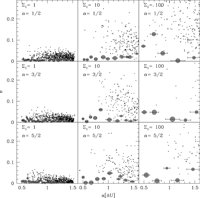
Figure 3: Figure 14 from Leinhardt & Richardson (2005)⁵⁷ showing their distributions of embryos and smaller bodies with a range in surface density exponents $\alpha$ and surface densities $\Sigma_{1}$ . All panels are at 500,000 years, except for panel 3 in rows 1 and 3 which are at 110,000 and 225,000 years, respectively. The horizontal bars represent 10 times the Hill radii.This figure was cited from Leinhardt & Richardson, Astrophys. J., 625, 427 (2005) with copyright permission from IoP publishers.

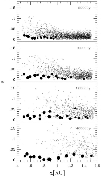
Figure 4: Snapshots in orbital eccentricity $e$ vs. semimajor axis $a$ in simulations of the growth of planetary embryos ⁵⁶. The radius of each particle is proportional to the simulation radius but is not to scale on the x axis.This figure was cited from Kokubo and Ida, Astrophys. J. 581, 666. (2002) with copyright permission from IoP publishers.

Figure 4 shows snapshots in time of a simulation of the formation of planetary embryos from planetesimals near 1 AU ⁵⁶. Accretion proceeds faster in the inner disk, such that the outer disk is still dominated by planetesimals when embryos are fully-formed in the inner disk. Oligarchic growth tends to form systems of embryos with roughly comparable masses and separations of 5-10 mutual Hill radii ⁵⁴, ⁵⁵, ⁵⁸. The details of the embryo distribution depend on the total mass and surface density distribution of the disk ⁵⁶. Typical embryo masses in a solar nebula model are a few percent of an Earth mass, i.e., roughly lunar to Mars-sized ⁵⁵, ⁵⁹. Figure 3 shows nine distributions of embryos with a range in surface densities exponents $\alpha$ and surface densities $\Sigma_{1}$ (see Eqn. 1 of Leinhardt and Richardson⁵⁷). For surface density profiles steeper than $r^{-2}$, the embryo mass decreases with orbital distance. Embryo masses scale roughly linearly with the local disk mass, and formation times are much faster for more massive disks.

The process of embryo formation via runaway and oligarchic growth has very recently come into question for three reasons. First, disk turbulence increases the random velocities of planetesimals, often above the critical disruption threshold for km-sized planetesimals. The capacity of planetesimals to survive collisions is represented in terms of of $Q_{D}^{*}$, the specific energy required to gravitationally disperse half of the object’s mass ⁶⁰, ⁶¹. For collisions more energetic than $Q_{D}^{*}$, collisions are erosive rather than accretionary making it difficult for embryos to grow. In the presence of MRI(magneto-rotational instability) -driven turbulence ⁶², accretionary growth of large bodies appears to require that larger bodies with higher $Q_{D}^{*}$ already exist ⁶³. The critical size of these large bodies is 300-1000 km. Second, new collision models suggest that planetesimals are weaker than previously estimated, such that accretion requires either very slow collisions or pre-seeding of the disk with larger objects ⁶⁴. Third, statistical models that attempt to reproduce the asteroid belt’s observed size distribution must also resort to seeding the region with large objects of at least 100 km in size ⁶⁵. These three lines of evidence all suggest that large, 100-1000 km bodies may have been required for the accretionary growth of the much larger embryos. This paradox could be resolved if planetesimals form via the turbulent concentration plus gravitational collapse model of Johansen et al. (2007)Johansen2007 ⁹, who inevitably formed 1000 km-scale bodies in MRI-turbulent disks.

3 Late-Stage Growth of the Terrestrial Planets

The planetary embryos formed during the previous oligarchic growth phase begin to perturb one another once the local mass in planetesimals and embryos is comparable ¹³. The orbital eccentricities of embryos become excited, which leads to a phase of close encounters and collisions with moderate velocities. Thus begins the final stage of terrestrial planet formation, which ends with the formation of a few massive planets. ⁶⁶, ⁶⁷, ⁶⁸, ⁶⁹, ⁷⁰. The duration of this phase is shortened through the presence of Jupiter, which increases the eccentricities of the embryos’ orbits and hence the mutual collision rates.

Wetherill (1992)Wetherill1992 ⁷¹ was the first to suggest that the formation of planetary embryos was not necessarily limited to the terrestrial planet region. He proposed that planetary embryos formed also in the asteroid belt. The mutual perturbations among the embryos, combined with the perturbations from Jupiter, would have eventually removed all the embryos from the asteroid belt, leaving in that region only a fraction of the planetesimal population on dynamically excited orbits. For this reason, some of the simulations of Chambers and Wetherill (1998) Chambers1998 ⁶⁸ started with a population of embryos ranging from $\sim$0.5 to $\sim$4 AU.

Most recent simulations take advantage of fast symplectic integrators such as Mercury⁷² or SyMBA⁷³. These integrators are optimized for planetary studies, and employ algorithms that allow for roughly 10 times fewer time steps per orbit as compared with a brute-force N-body integrator, for the same accuracy. These integrators also allow for close encounters between bodies, either by numerically solving the interaction component of the Hamiltonian (Mercury) or by recursively subdividing the time step (SyMBA). When performing integrations with these codes, it is always important to choose a time step that is small enough to resolve the orbits of the innermost particles with at least $\sim$ 20 time steps per orbit to avoid numerical errors ⁷⁴, ⁷⁵. Collisions are generally modeled in a very simplistic fashion, as inelastic mergers occurring anytime two bodies touch. Although this assumption appears absurd, it has been shown to have little to no effect on the outcome of accretion simulations ⁷⁶. However, more complex models show that dynamical friction from collisional debris may play an important role at late stages ⁷⁷.

A convenient approximation is often made to reduce the run time needed per simulation, by neglecting graviational interactions between planetesimals (see Raymond et al. (2006)for a discussion of this issue)⁷⁸. Assuming that planetesimals do not interact with each other, the run time $\tau$ scales with the number of embryos $N_{e}$ and the number of planetesimals, $N_{p}$, roughly as $\tau\sim N_{e}^{2}+2N_{e}N_{p}$. The non-interaction of planetesimals eliminates an additional $N_{p}^{2}$ term. Note that $\tau$ refers to the computing time needed for a given timestep. The total runtime is $\tau$ integrated over all timesteps for all surviving particles. Thus, a key element in the actual runtime of a simulation is the mean particle lifetime. Configurations with strong external perturbations (e.g., eccentric giant planets) tend to run faster because the mean particle lifetime is usually shorter than for configurations with weak external perturbations.

Tree codes, which subdivide a group of particles into cells using an opening angle criterion, have the advantage over serial codes in that the run time scales with particle number $N$ as $NlogN$ rather than $N^{2}$. They can be run in parallel on several CPUs to further reduce the runtime. Tree codes have been used to study planetary dynamics, but to date are only useful in the regime of large $N$ ($N\gtrsim 10^{4}$;⁷⁹). The reason for this is that a large amount of computational ”overhead” is required to build the tree, such that for small $N$ more computing time is needed for building the tree, and if run in parallel, for communication between processors. The break-even point between serial codes and tree codes, for example, is at $N\sim 1000$⁸⁰. An advantageous hybrid method for large $N$ accretion simulations is to integrate particles’ orbits with a parallel tree code until $N$ drops to about 1000, then switch to serial code for the rest of the simulation⁸¹.

A common problem with the current generation simulations is that the final terrestrial planets are on orbits that are too eccentric and inclined with respect to the real orbits. The orbital excitation is commonly quantified by the normalized angular momentum deficit⁸²:

$$AMD=\frac{\sum_{j}m_{j}\sqrt{a_{j}}\left(1-cos(i_{j})\sqrt{1-e_{j}^{2}}\right)}{\sum_{j}m_{j}\sqrt{a_{j}}},$$ (2)

where $a_{j}$, $e_{j}$, $i_{j}$, and $m_{j}$ refer to planet $j$’s semimajor axis, eccentricity, inclination with respect to a fiducial plane, and mass. The $AMD$ of the Solar System’s terrestrial planets is 0.0018. For comparison, the Chambers and Wetherill (1998) Model C simulations, each consisting of at most  50 bodies extending out to 4 AU and assuming the present orbits of Jupiter and Saturn, yield a median AMD of -0.033. The Chambers (2001) simulations 21-24, each consisting of about 150 bodies and also assuming the present Jupiter and Saturn, have a median AMD of -0.0050. Those simulations only extended out to 2 AU, and it is likely that their AMD would be even higher if they were extended out to 4 AU (e.g., the Chambers and Wetherill (1998) Model C Simulations, which extend out to 4 AU, have a median AMD about 50% larger than in their Model B simulations, which only extend to 1.8 AU).

The missing physics responsible for this mismatch between simulations and constraints is an open subject of scientific debate. It has been proposed ⁸³, ⁸⁴ that a remnant fraction of the primordial nebula would have damped the eccentricities and inclinations of the growing planets. In this case, however, the simulations typically form systems of planets that are too numerous and too small. The work has been extended by including the effects of secular resonance sweeping as the solar nebula dissipates ⁸⁵, ⁸⁶. This both forces mergers to reduce the number of final terrestrial planets to be comparable to our Solar System, and shortens the growth timescale so that there is sufficient nebular gas at the finish to damp the eccentricities to match those of the Solar System terrestrial planets.The MHD turbulence of the nebula might also alleviate the problem, enhancing the probability that the proto-planets collide with each other and thus leading to systems with a smaller number of larger planets ⁸⁷. A problem with both of these scenarios, however, is that since they occur on the timescale comparable to the existence of the nebular gas (a few to $\sim$10 Myr). This is not consistent with the significantly longer formation timescales inferred from isotopic chronometry of the Earth-Moon system ¹⁵, discussed more extensively at the end of this section.

Another possible way to reconcile the simulation results with the constraints is the inclusion of dynamical friction. Dynamical friction occurs if embryos and proto-planets evolve among a population of small planetesimals with a total mass comparable to the total mass of the embryos. A bi-modal distribution of embryos and planetesimals such as this is the likely result of oligarchic growth ⁴⁹, ⁵⁴. Dynamical friction produces the equipartition of the “excitation” energy (e.g., related to velocity dispersion, in analogy to the temperature of a gas) between gravitationally interacting bodies: the smaller ones obtain higher relative velocities, and the larger ones lower. The relative velocity of embryos (hence their eccentricities and inclinations) will therefore be kept low by dynamical friction. The simulation of a large number of small planetesimals is, of course, very CPU-intensive. Thus simulations typically neglect the effect of the small bodies, or include only a limited number of them, which are, therefore, artificially too massive.

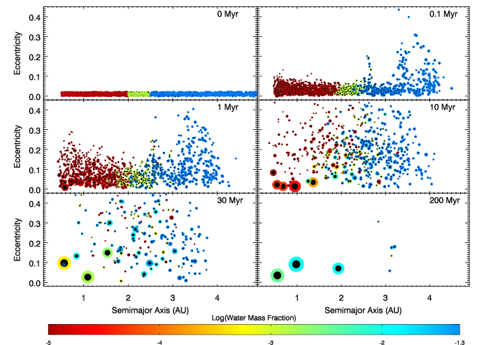
Figure 5: Snapshots in time from a simulation of the late-stage accretion of terrestrial planets, starting from 1885 sub-isolation mass objects ⁷⁸. The size of each body is proportional to its mass^1/3, the dark circle represents the relative size of each body’s iron core (in the black and white version, iron cores are shown only for bodies larger than 0.05 M${}_{\rm Earth}~{}$), and the color corresponds to its water content (red = dry, blue = 5% water). For a movie of this simulation, go to http://casa.colorado.edu/$\sim$raymonsn and click on “movies and graphics”.

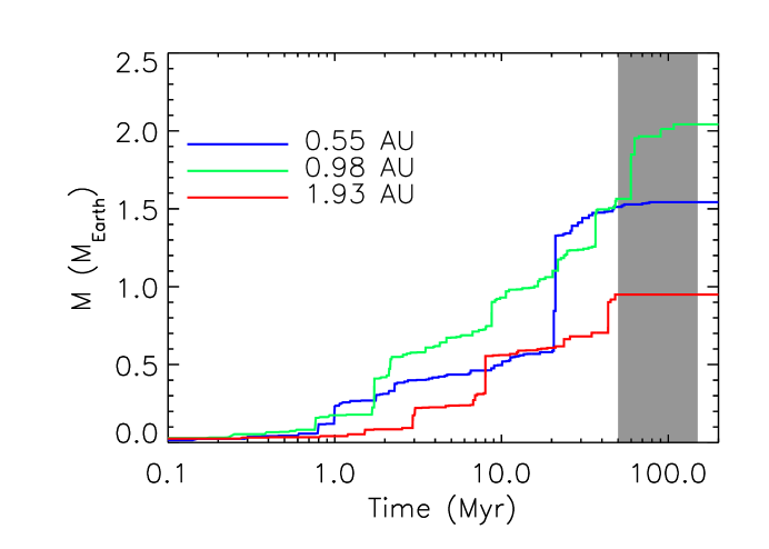
Figure 6: Growth of the three planets that formed in the simulation from Fig. 5 ⁷⁸, labeled by their final orbital distances. The shaded region shows the constraint from isotopic measurements for the timing of the Moon-forming impact ¹⁵.

An example evolution of an accretion simulation is shown in Figure 5 ⁷⁸. This simulation started with 1886 sub-embryo sized objects, and is one of the most computationally expensive to date, having required 1.2 x 10⁴ CPU hours. The simulation contains a single Jupiter-mass giant planet at 5.5 AU (not shown), and the evolution is characteristic of simulations with low-eccentricity giant planets. Eccentricities are excited in the inner disk by mutual scattering between embryos, and in the outer disk via resonant and secular forcing from the giant planet. Dynamical friction acts to keep the eccentricities of faster-growing embryos the smallest, and accretion proceeds from the inside of the disk outward. Only when embryos reach a critical size can they scatter planetesimals and other embryos strongly enough to cause large-scale radial mixing, which is evident in Fig. 5 by the change in colors (which represent water contents) of objects. The Earth analog in this simulation started to accrete asteroidal water only after $\sim$ 20 Myr of evolution, when it was more than half of its final mass. At the end of this simulation, three planets have formed: reasonable Venus and Earth analogs at 0.55 and 0.98 AU, and a much-too-massive Mars analog at 1.93 AU. Figure 6 shows the growth of the three planets in time. The accretion of the Earth analog occurs on the correct timescale, as it experiences its last giant impact at $t\approx 60$ Myr. The Venus and Mars analogs experience their final giant impacts at 22 and 40 Myr, respectively.

The comparison between the results in Chambers and Wetherill (1998)Chambers1998 ⁶⁸ (no small bodies included) and Chambers (2001)Chambers2001 ⁷⁰ (accounting for a bi-modal mass distribution in the initial population) suggested that dynamical friction is indeed important and can drive the simulation results in a good direction. Thus O’Brien et al. (2006)OBrien06 ⁸⁸ performed new simulations, starting from a system of 25 Mars-mass embryos from 0.5 to 4 AU, embedded in a disk of planetesimals with the same total mass and radial extent as the population of embryos, modeled with 1,000 particles. They performed two sets of four simulations. In one set, called ‘EJS’ for ‘Eccentric Jupiter and Saturn,’ Jupiter and Saturn are assumed to be initially on their current orbits, and in the second set, called ‘CJS’ for ‘Circular Jupiter and Saturn,’ they are assumed to be on nearly circular orbits with a smaller mutual separation.

The results of the EJS simulations, with Jupiter and Saturn initially on the current, eccentric orbits, can be compared directly to those of Chambers (2001) Chambers2001 ⁷⁰. The eccentricities and inclinations of the final terrestrial planets ⁸², ⁷⁰ measured through the AMD turn out to be five times smaller, on average, than in Chambers’ runs, and even $\sim$40% lower than in the real Solar System. The median time for the last giant impact is $\sim$30 Myr. For comparison, while Chambers (2001) Chambers2001 ⁷⁰ does not report the time of last giant impact, his Earth and Venus analogues take 54 and 62 Myr, respectively, to reach 90% of their final mass. (A recent study by one of the authors (SNR) and his colleagues suggest a spread of a factor of a few, and sometimes larger, between the last giant impact on Earth analogs in different simulations with the same set of initial conditions but different random number initializations).

The CJS simulations, with Jupiter and Saturn initially on quasi-circular orbits and with smaller mutual separations, give a median time for the last giant collision of about 100 Myr. They still give terrestrial planets that are a bit too dynamically excited. The eccentricities and inclinations, as measured by the AMD, are about 60% larger on average than those of the real terrestrial planets. These somewhat unsatisfactory results with regards to dynamical excitation do not imply necessarily that Jupiter and Saturn had to have their current orbits when the process of terrestrial planet formation started. The spectacular improvement in the results between the runs in Chambers (2001)Chambers2001 ⁷⁰ and the EJS simulations in O’Brien et al. (2006)OBrien06 ⁸⁸ demonstrates the dramatic effect of dynamical friction on reducing planetary excitation. With only 1,000 particles used to simulate the planetesimal disk, there is no reason to think that the simulations by O’Brien et al. (2006)OBrien06 ⁸⁸ give a fully accurate treatment of dynamical friction. Thus, it is possible that a future generation of simulations, using more particles of smaller individual mass to model the planetesimal disk, and allowing for the regeneration of planetesimals when giant impacts occur between embryos⁷⁷, would treat dynamical friction more accurately and lead to satisfactory results even with Jupiter and Saturn starting on circular orbits.

Several statistical quantities exist to compare the properties of a system of simulated terrestrial planets with the actual inner Solar System⁷⁰. These include the number and masses of the planets, their formation timescales, the AMD of the system, and the radial concentration of the planets (the vast majority of the terrestrial planets’ mass is concentrated in an annulus between Venus and Earth). Reproducing all observed constraints in concert is a major goal of this type of research⁸⁹.

With respect to formation timescales, constraints are available from measurement of radioactive isotopic systems in rocks on the Earth and Moon. To date these have yielded conflicting results. A very detailed analysis¹⁵, uses these chronometers, the identity of the tungsten isotopic ratios in the Moon and the Earth’s mantle, and isotopic dating of the oldest moon rocks. They conclude that the last giant impact–that which formed the Earth’s Moon–occurred between 50-150 million years after the appearance of the first solids in the protoplanetary disk which formed the solar system. We assume–but cannot demonstrate– that this giant impact did not occur a significant fraction of the Earth-formation time later than the collisions that built the Earth to its present size. With that in mind, we argue that any simulations which grow the Earth on a timescale roughly between a few tens of millions and 150 million years are consistent with the indications from the geochemical data.

With respect to the radial distribution of terrestrial planet mass, the simulations described above start with a power law column density of solids. In contrast, Chambers and Cassen (2002)Chambers2002 ⁹⁰ simulated late-stage accretion by generating embryos from the detailed disk model of Cassen (2001)Cassen01 ⁹¹ which contains a peak in the surface density at 2 AU (in that model, $\Sigma\propto a$ for $a<$ 2 AU, and $\Sigma\propto a^{-0.3}$ for $a>$ 2 AU). They found that simulations with embryos generated from a standard MMSN model did a much better job of reproducing the properties of the terrestrial planets than the more detailed theoretical disk model. Jin et al. (2008) Jin08 ⁹² created a disk model with multiple zones, assuming that the ionization fraction of the gas varied radially, thereby affecting the local viscosity and causing pileups and dearths of gas at the boundaries between zones. They suggested that non-uniform embryo formation in such a disk could explain Mars’ small size. Preliminary simulations by one of the authors (S.R.) and colleagues have called into question this suggestion.

3.1 Delivery of Water-Rich Material from the Asteroid Belt

An outstanding application of the dynamical models is to the problem of the origin of Earth’s water. The oceanic water content of the Earth is about 0.02% the mass of the Earth, and various geochemical estimates put the total amount of water that was present early in the Earth’s history at 5-50 times this number, some or all of which may yet reside in the mantle ⁹³. However, meteoritic evidence and theoretical modeling suggest that the protoplanetary disk at 1 AU was too warm at the time the gas was present to allow condensation of either water ice or bound water. Therefore, there has been a longstanding interest in models that deliver water ice or water-rich silicate bodies to the Earth during the latter’s formation. Much of the isotopic and dynamical evidence against cometary bodies being a primary source, oft quoted in the literature, has been reviewed recently ⁹⁴, and a comprehensive treatment of the geochemical evidence is beyond the scope of this review. Likewise, alternative models for local delivery of water, for example in the form of adsorbed water on nebular silicate grains ⁹⁵ have been proposed, but will not be described. Of interest here is how the dynamical models described above can be used to quantify the delivery of large bodies to the Earth from the asteroid belt, where chondritic material (in the form of meteorites) has an average $D/H$ ratio close to that of the Earth’s oceans.

The fact that the $D/H$ ratio of Earth’s water is chondritic prompted Morbidelli et al. (2000)Morby2000 ⁹⁶ to look at dynamical models of terrestrial planet formation to investigate whether a sufficiently large amount of mass could be accreted from the asteroid belt. They used simulations from Chambers and Wetherill (1998)Chambers1998 ⁶⁸, in which planetary embryos beyond 2 AU had several times the mass of Mars, and two new simulations with a larger number of individually smaller embryos (masses ranging from a lunar mass at $\sim$1 AU to a Mars mass at $\sim$4 AU). They found that 18 out of the 24 planets formed in the simulations accreted at least one embryo originally positioned beyond 2.5 AU. When this happened, at least $\sim$10% of the final planet mass was accreted from this source. Assuming that the embryos originally beyond 2.5 AU had a composition comparable to that of carbonaceous chondrites (namely with 5 to 10% of mass in water), they concluded that these planets would be “wet’, i.e. they would start their geochemical evolution with a total budget of about 10 ocean masses of water or more. Moreover, Morbidelli et al. (2000)Morby2000 ⁹⁶ also studied the evolution of planetesimals under the influence of the embryos. They found that planetesimals from the outer asteroid belt also contribute to the delivery of water to the forming terrestrial planets, but at a considerably minor level with respect to the embryos. They also found that comets from the outer planet region could bring no more than 10% of an ocean mass to the Earth, because the collision probability of bodies on cometary orbits with the earth is so low. From all these results, they concluded that the accretion of a large amount of water is a stochastic process, depending on whether collisions with embryos from the outer asteroid belt occur or not. Thus, they envisioned the possibility that in the same planetary system some terrestrial planets are wet, and others are water deficient.

The findings of Morbidelli et al. (2000)Morby2000 ⁹⁶ have been confirmed in a series of subsequent works⁹⁷, ⁹⁸, ⁷⁸. In particular, with simulations starting from a larger number of smaller embryos, Raymond et al. (2007)Raymond2007 ⁹⁹ concluded that the accretion of a large amount of water from the outer asteroid belt is a generic result, and argued that the fact that 1/3 of the planets in Morbidelli et al. (2000)Morby2000 ⁹⁶ were dry was an artifact of small number statistics due to the limited number of embryos used in those simulations.

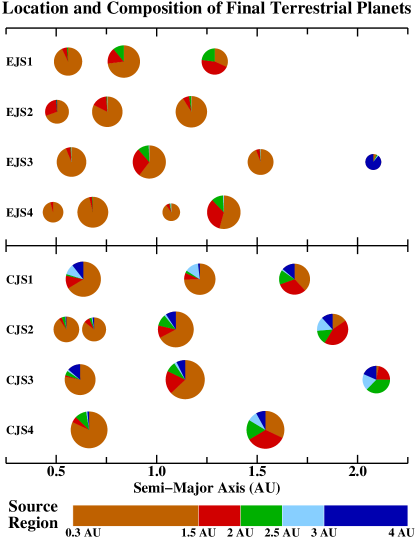
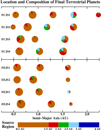
Figure 7: Final terrestrial planets formed in the O’Brien et al. (2006) OBrien06 ⁸⁸ simulations (EJS and CJS) as well as the ECJS and EEJS ⁸⁹ simulations discussed in the text. Pie-diagrams show the relative contribution of material from the different semi-major-axis regions, and the diameter of each symbol is proportional to the diameter of the planet.

Figure  7 shows the origin of the material incorporated in the final terrestrial planets in the O’Brien et al. (2006)OBrien06 ⁸⁸ simulations. The top panel concerns the set of four simulations with Jupiter and Saturn initially on circular orbits, and the middle panel to the set with giant planets initially on the current orbits. Each line refers to one simulation. Each planet is represented by a pie diagram, with size proportional to the planet’s diameter and placed at its final semi-major axis. The colors in each pie show the contributions of material from the different semimajor-axis regions shown on the scale at the bottom of the figure. This represents the feeding zone of each planet. The feeding zones are not static, but generally widen and move outward in time⁷⁸.

An important difference is immediately apparent between the two sets of simulations. In the set with Jupiter and Saturn initially on circular orbits, an important fraction of the mass of all terrestrial planets comes from beyond 2.5 AU, and would likely be water-bearing carbonaceous material. About 75% of this mass is carried by embryos, the remaining part by planetesimals. Thus, the idea that the water comes predominantly from the asteroid belt is supported. However, in the set of simulations with giant planets initially on their current, eccentric orbits, none of the planets accretes a significant amount material from beyond 2.5 AU. In that case, if the asteroid belt is the source of water, it would have to be through objects of ordinary chondritic nature, typical of its inner part. We will come back to this idea below. This dramatic difference between the cases with eccentric or circular giant planets had already been suggested⁹⁰, and is explained by several authors⁹⁷,¹⁰⁰, and⁸⁸.

Thus, a crucial question for the origin of the Earth’s water is whether it is more reasonable to assume that the giant planets initially had eccentric or circular orbits. The core of a giant planet is expected to form on a circular orbit because of strong damping by dynamical friction and tidal interactions with the gas disk ⁴⁹, ¹⁰¹, ¹⁰², ¹⁰³.

Once an isolated giant planet is formed, if the mass is less than about 3 Jupiter masses, its interactions with the gas disk should not raise its orbital eccentricit¹⁰⁴ (but see Goldreich and Sari (2003)Goldreich2003 ¹⁰⁵), but rather damp it out, if it is initially non-zero. In our Solar System, however, we don’t have an isolated giant planet, but two. The dynamics of the Jupiter-Saturn pair has been investigated¹⁰⁶, ¹⁰⁷, ¹⁰⁸. A typical evolution is that Saturn becomes locked into the 2:3 resonance with Jupiter. This case is appealing because it may prevent Jupiter from migrating rapidly towards the Sun, thus explaining why our Solar System does not have a hot giant planet. Even in the case of 2:3 resonance locking, the orbital eccentricity of the giant planets remain small. The eccentricity of Jupiter does not exceed 0.007. There are, however, a few cases in which the eccentricity of the giant planets can grow¹⁰⁷. For instance, if a fast mass accretion is allowed onto the planets, the resonance configuration can be broken, and the eccentricity of Jupiter can temporarily grow to $\sim$0.1. Also, if the planets are locked into the 3:5 resonance, the eccentricity of Jupiter can be raised to 0.035, which is close to its current value. All these cases, however, are unstable and temporary, so one has to invoke the disappearance of the disk at the time of the excitation, otherwise the planets would find another more stable configuration and the disk would damp the eccentricities back to very small values. So, according to our (limited) understanding of giant planet formation and gas-disk interactions, a very small orbital eccentricity seems to be more plausible, but an eccentric orbit cannot be ruled out with absolute confidence.

What seems more secure, conversely, is that when the terrestrial planet formation process began, the orbits of Jupiter and Saturn had to have a smaller mutual separation than their current value. In fact, all simulations agree in showing that the interaction of the giant planets with the massive planetesimal disk that would have existed in the early outer Solar System leads to a significant amount of radial migration ¹⁰⁹, ¹¹⁰, ¹¹¹. In particular, Saturn, Uranus and Neptune migrate outwards, whereas Jupiter migrates inwards. Thus, the orbital separation between Jupiter and Saturn grows with time. Recently, a model of the evolution and delayed migration of the giant planets has been proposed, and it reproduces fairly well the current architecture of the outer solar system¹¹², ¹¹³. This “Nice” model assumes that Jupiter and Saturn were initially interior to their mutual 1:2 mean motion resonance (MMR), and that the orbits of the giant planets at the time they cross their 2:1 MMR were nearly circular. Giant planet migration and the crossing of the 2:1 resonance could be delayed for hundreds of Myr, such that the initial configuration would last for the entirety of the terrestrial planet formation process¹¹³. The second assumption of circular orbits at the time of the resonance crossing does not dismiss, in principle, the simulations of terrestrial planet formation starting with Jupiter and Saturn on eccentric orbits, because, in these simulations, the giant planets eccentricities are damped very fast by the ejection of material from the Solar System and meet the requirements of Tsiganis et al. (2005)¹¹² and Gomes et al. (2005)¹¹³ model after a few tens of Myr. One should explain in this case, though, where such eccentricity comes from. Conversely, the first assumption of a smaller initial orbital orbital separation of Jupiter and Saturn is essential for the success of that model.

For these reasons, we have performed a new set of four simulations, where Jupiter and Saturn are assumed to have initially the current orbital eccentricities, and an orbital separation consistent with the Tsiganis et al. (2005)¹¹² and Gomes et al. (2005)¹¹³ model. The results in terms of final eccentricities and inclinations of the terrestrial planets and accretion timescales are intermediate between those of the two sets of simulations in O’Brien et al. (2006)OBrien06 ⁸⁸ discussed above with AMD values consistent with the Solar System values and a formation timescale consistent with the Hf-W age of the Earth-Moon system¹⁵. The origin of the mass accreted by the terrestrial planets is presented in the bottom strips of Fig. 7. The planets at or beyond 1 AU, with only one exception, receive an important mass contribution from the outer asteroid belt, that is comparable to, if not larger, than that from the inner belt. The planets inside 1 AU typically do not receive a significant mass contribution from the outer belt, and the contribution from the inner belt is also very moderate.

We believe that we understand, at least at a qualitative level, the differences between the results of these new runs and those of the set of O’Brien et al. (2006) ⁸⁸ with Jupiter and Saturn on their current orbits, in which none of the planets recieved significant outer-belt material. If the orbits of the giant planets are closer to each other, the planets precess faster. Thus the positions of the secular resonances are shifted outwards. In particular, the powerful $\nu_{6}$ resonance (occurring when a body’s perihelion precesses at the same rate as Saturn’s), which is currently at the inner border of the belt, moves beyond the outer belt. The $\nu_{6}$ resonance can drive objects onto orbits with $e\sim 1$, such that they are eliminated by collision with the Sun. It is therefore an obstacle to the transport of embryos from the asteroid belt into the terrestrial planet region. In fact, in decreasing their semi-major axes from main belt-like values to terrestrial planets-like values, the embryos in the EJS simulation have to pass through the resonance. Of course, collisions with the growing terrestrial planets are also possible for objects with a Main Belt-like semi-major axis and a large eccentricity, but they are less likely. An embryo can be extracted from the resonance by an encounter with another embryo, but this is also an event with a moderate probability. So, the flux of material from the belt to the terrestrial planet region is enhanced if the $\nu_{6}$ resonance is not present. This is the case if the eccentricities of the planets are zero as in the CJS simulations (in this case the resonance vanishes), or if the planets are closer to each other as in the ECJS simulations (in which case the resonance is active, but it is not between the terrestrial planets region and the asteroid belt). In the ECJS simulations, the $\nu_{6}$ is located around 3.4 AU. We stress that, in order to move the $\nu_{6}$ resonance beyond the asteroid belt, it is not necessary that Jupiter and Saturn are as close as postulated in the Tsiganis et al. (2005) ¹¹² and Gomes et al. (2005) ¹¹³ model. The initial, less extreme, orbital separations used in other models ¹¹⁰, ¹¹¹ would give a similar result.

We have recently performed several additional sets of simulations ⁸⁹, including the EEJS (‘Extra-Eccentric Jupiter and Saturn’) set. In four EEJS simulations, Jupiter and Saturn were placed at their current semimajor axes but with starting eccentricities of 0.1. These systems therefore experienced very strong perturbations from the $\nu_{6}$ resonance at 2.1 AU, which acted to remove material from the Mars region and also to effectively divide the inner Solar System from the asteroid belt. These simulations were the first to produce reasonable Mars analogs, but suffered in terms of water delivery to the Earth. Scattering of embryos and planetesimals during accretion decreased Jupiter and Saturn’s eccentricities to close to their current values, but the EEJS system does not allow for any delayed giant planet migration as may be required by models of the resonant structure of the Kuiper belt ¹¹⁴, ¹¹⁵. In fact, it is important to note that the EJS simulations described above are absolutely inconsistent with the Solar System’s architecture because accretion damps the eccentricities of Jupiter and Saturn to below their current values, and there is no clear mechanism to increase them without affecting their semimajor axes.

In conclusion, the simulations seem to support, from a dynamical standpoint, the idea of the origin of water on Earth from the outer asteroid belt. However, the stochasticity of the terrestrial planet accretion process, the limitations of the simulations that we have used, and the uncertainties on the initial configuration of the giant planets do not allow us to exclude a priori the possibility that the Earth did not receive any contribution from the outer asteroid belt, whereas it accreted an important fraction of its mass from the inner belt or its vicinity. For this reason, geochemical evidence has been used to try to constrain where the Earth’s water came from. For example ¹¹⁶ have argued that (a) oxygen isotopic differences and (b) siderophile element patterns limit the carbonaceous chondritic contribution to 1% of the mass of the Earth. Constraint (a) can be removed or relaxed if the oxygen isotope composition of the Earth and the putative chondritic impactor were homogenized in the manner proposed for the Moon-forming impact event ¹¹⁷. (For the Moon-forming impactor such a process is deemed essential because the Earth and Moon have identical isotopic ratios for both oxygen and tungsten, whereas meteorites vary from these ratios). Constraint (b) is a strong one only for relatively small bodies delivering water in a late veneer of material, or undifferentiated chondritic embryos mixing fully with the Earth’s mantle during the main growth phase. If the embryo that delivered the water were differentiated then its core, containing most of the siderophile elements, would not mix with the Earth’s mantle.

4 Extrapolation to Extrasolar Terrestrial Planet Systems

What counts for terrestrial planet formation? The key parameters are 1) the disk mass and radial density distribution, and 2) the giant planet properties (mass, orbit, migration). Here we summarize some relevant issues see ¹¹⁸ for a more detailed review:

• Effect of Disk Properties The accreted planet mass is slightly more than linearly proportional to the disk mass because the planetary feeding zone widens with disk mass due to stronger embryo-embryo scattering ¹¹⁹, ¹²⁰. However, planets that grow to more than a few Earth masses during the gaseous disk phase may accrete a thick H/He envelope and be “mini-Neptunes” rather than “super Earths” ¹²¹, ¹²² . Whether such objects might be among the super-Earth mass planets observed around other stars is an interesting but as yet ill-constrained speculation.

  The disk’s surface density profile is another key factor. For steeper density profiles, the terrestrial planets form faster and closer to the star, are more massive, more iron-rich and drier than planets that form in disks with shallower density profiles ⁹⁸. Disks around other stars are observed to have somewhat shallower density slopes¹²³, ¹²⁴ than the $r^{-3/2}$ minimum-mass solar nebula model of Hayashi (1981)Hayashi1981 ¹²⁵ and Weidenschilling (1977) Weidenschilling1977 ¹²⁶. However, given the preponderance of evidence that giant planets migrate, the validity of the minimum-mass solar nebula for either our own solar system or other planetary systems is called into question ¹²⁷, ¹²⁸. Well-resolved observations of disk surface density profiles from facilities like ALMA will help resolve this in the near future.

• Low-Mass Stars. Low-mass stars are in some sense an ideal place to look for Earth-like planets, because an Earth-mass planet in the habitable zone induces a stronger radial velocity signal in the star on a much shorter period than for a Sun-like star ¹²⁹, ¹³⁰. However, sub-mm observations of the outer portions of dusty disks around young stars show a roughly linear correlation between disk mass and stellar mass, with a scatter of about 2 orders of magnitude in disk mass for a given stellar mass ¹³¹, ¹³², ¹³³. Thus, low-mass stars tend to have low-mass disks which should therefore form low-mass giant ¹³⁴ and terrestrial planets ¹²⁰. However, several low-mass stars are observed to host massive (several Earth-mass), close-in planets ¹³⁵, ¹³⁶.

• Effect of Giant Planet Properties. Compared with a standard case that includes giant planets exterior to the terrestrial planet forming region, the following trends have been noted in dynamical simulations: 1) More massive giant planets lead to fewer, more massive terrestrial planets ¹³⁷, ⁹⁷; 2) More eccentric giant planets lead to fewer, drier, more eccentric terrestrial planets ⁹⁰, ¹³⁷, ⁹⁷, ¹⁰⁰, ⁸⁸. Giant planets have a negative effect on water delivery in virtually all cases, overly-perturbing and ejecting much more water-rich asteroidal material than they allow to slowly scatter inwards (S. Raymond, unpublished data).

  Hot Jupiter systems represent an interesting situation. In these systems, the giant planet is thought to have formed exterior to the terrestrial planet zone, then migrated through that zone ¹³⁸. Recent simulations have shown that the giant planet’s migration actually induces the formation of rocky planets in two ways: 1) interior to the giant planet, material is shepherded by mean motion resonances, leading to the formation of very close-in terrestrial planets ¹³⁹, ¹⁴⁰, ¹⁴¹, ¹⁴², ¹¹⁸, ¹⁴³; and 2) exterior to the giant planet, the orbits of scattered embryos are re-circularized by gaseous interactions leading to the formation of a second generation of extremely water-rich terrestrial planets at $\sim$ 1 AU ¹⁴², ¹⁴³. Hence, a key factor is the chronology of migration vs. disk dispersal. If the migration happens when there is still a lot of mass in the disk for a good amount of time, then scattered material can be saved and planets can formed.

5 Conclusion

Simulation of terrestrial planet formation has become a mature subfield of dynamical astronomy, with the potential to provide insight into the origin of our own solar system as well as that of the increasing number of multiple planet systems being discovered beyond our solar system. Further progress certainly will come from faster computers employing novelties such as, for example, many CPUs on a given chip allowing for easy communication between processors and improved performance and relevance of parallel codes. But additional insight into the physics and chemistry of the problem will be required as well. For example, while the general nature of our terrestrial planet system seems to be broadly reproduced by the models, still unexplained is the presence of an embryo-sized body, Mars, in place of the more massive objects that the simulations tend to yield. Are such outcomes common? We cannot answer this question with the current state of maturity of the field.

Another issue is the effect that collisions between embryos and the growing terrestrial planets have on the geochemistry of the latter. The challenge of quantifying in detail the chemical and physical processes that occur during giant impacts is a problem outside the scope of the dynamical modeling described here, but crucial in trying to relate the geochemistry of the Earth and other terrestrial planets to the source material from which they grew. Close collaboration between groups that specialize in these two very different types of numerical simulations may permit more detailed and confident geochemical predictions in the future. And this, in turn, will increase our confidence in the predictions the models described herein can make for the properties of terrestrial planets around stars other than our own.

6 Acknowledgements

We thank Anders Johansen, Eiichiro Kokubo, and Zoe Leinhardt for their contributed figures. S.N.R. is grateful for funding from NASA’s Origins of Solar Systems program (grant NNX09AB84G) and the Virtual Planetary Laboratory, a NASA Astrobiology Institute lead team, supported by NASA under Cooperative Agreement No. NNH05ZDA001C. This paper is PSI Contribution 461.

.

References

- [1] V. S. Safronov, Evoliutsiia doplanetnogo oblaka. (1969., 1969).
- [2] S. Weidenschilling, Icarus 22, 426 (1976).
- [3] Y. Nakagawa, K. Nakazawa, C. Hayashi, Icarus 45, 517 (1981).
- [4] G. W. Wetherill, Ann. Rev. Astr. Ap. 18, 77 (1980).
- [5] R. Greenberg, W. K. Hartmann, C. R. Chapman, J. F. Wacker, Icarus 35, 1 (1978).
- [6] G. W. Wetherill, G. R. Stewart, Icarus 77, 330 (1989).
- [7] P. Goldreich, W. R. Ward, Astrophys. J. 183, 1051 (1973).
- [8] J. N. Cuzzi, R. C. Hogan, K. Shariff, Astrophys. J. 687, 1432 (2008).
- [9] A. Johansen, et al., Nature 448, 1022 (2007).
- [10] S. Ida, J. Makino, Icarus 96, 107 (1992).
- [11] S. Ida, J. Makino, Icarus 98, 28 (1992).
- [12] G. W. Wetherill, Science 228, 877 (1985).
- [13] S. J. Kenyon, B. C. Bromley, Astron. J. 131, 1837 (2006).
- [14] K. E. Haisch, Jr., E. A. Lada, C. J. Lada, Astrophys. J. Lett. 553, L153 (2001).
- [15] M. Touboul, T. Kleine, B. Bourdon, H. Palme, R. Wieler, Nature 450, 1206 (2007).
- [16] B. Reipurth, D. Jewitt, K. Keil, Protostars and Planets V (University of Arizona Press, Tucson, 2007).
- [17] J. Najita, S. Strom, J. Muzerolle, Mon. Not. R Astron. Soc. 378, 369 (2007).
- [18] F. Moynier, Q.-z. Yin, B. Jacobsen, Astrophysical Journal 671, L181 (2007).
- [19] I. Adachi, C. Hayashi, K. Nakazawa, Progress of Theoretical Physics 56, 1756 (1976).
- [20] J. Chambers, Icarus 180, 496 (2006).
- [21] C. P. Dullemond, C. Dominik, A&A 434, 971 (2005).
- [22] S. J. Weidenschilling, J. N. Cuzzi, Protostars and Planets III, E. H. Levy, J. I. Lunine, eds. (University of Arizona Press, Tucson, AZ, 1993), pp. 1031–1060.
- [23] A. N. Youdin, F. H. Shu, Astrophys. J. 580, 494 (2002).
- [24] G. Wurm, J. Blum, Astrophys. J. Lett. 529, L57 (2000).
- [25] T. Poppe, J. Blum, T. Henning, Astrophys. J. 533, 454 (2000).
- [26] W. Benz, Space Science Reviews 92, 279 (2000).
- [27] C. Dominik, A. G. G. M. Tielens, Astrophys. J. 480, 647 (1997).
- [28] J. N. Cuzzi, A. R. Dobrovolskis, J. M. Champney, Icarus 106, 102 (1993).
- [29] J. N. Cuzzi, C. M. O. Alexander, Nature 441, 483 (2006).
- [30] C. P. Dullemond, C. Dominik, A&A 421, 1075 (2004).
- [31] S. J. Weidenschilling, Monthly Not. Roy. Astron. Soc. 180, 57 (1977).
- [32] S. J. Weidenschilling, Space Science Reviews 92, 295 (2000).
- [33] V. Safronov, Annales d’Astrophysique 23, 979 (1960).
- [34] J. N. Cuzzi, R. C. Hogan, J. M. Paque, A. R. Dobrovolskis, Astrophys. J. 546, 496 (2001).
- [35] W. K. M. Rice, G. Lodato, J. E. Pringle, P. J. Armitage, I. A. Bonnell, Monthly Not. Roy. Astron. Soc. 372, L9 (2006).
- [36] J. N. Cuzzi, A. R. Dobrovolskis, R. C. Hogan, Chondrules and the Protoplanetary Disk (1996), pp. 35–43.
- [37] N. Haghighipour, A. P. Boss, Astrophys. J. 598, 1301 (2003).
- [38] A. Johansen, H. Klahr, T. Henning, Astrophys. J. 636, 1121 (2006).
- [39] A. N. Youdin, J. Goodman, Astrophys. J. 620, 459 (2005).
- [40] A. Johansen, A. Youdin, Astrophys. J. 662, 627 (2007).
- [41] J. Goodman, B. Pindor, Icarus 148, 537 (2000).
- [42] P. Tanga, A. Babiano, B. Dubrulle, A. Provenzale, Icarus 121, 158 (1996).
- [43] P. Barge, J. Sommeria, Astronomy and Astrophysics 295, L1 (1995).
- [44] H. B. Throop, J. Bally, Astrophys. J. Lett. 623, L149 (2005).
- [45] Y. Greenzweig, J. J. Lissauer, Icarus 100, 440 (1992).
- [46] Y. Greenzweig, J. J. Lissauer, Icarus 87, 40 (1990).
- [47] V. Safronov, Evolution of the Protoplanetary Cloud and Formation of the Earth and Planets (NASA TTF-677, 1972).
- [48] G. W. Wetherill, G. R. Stewart, Icarus 106, 190 (1993).
- [49] E. Kokubo, S. Ida, Icarus 123, 180 (1996).
- [50] P. Goldreich, Y. Lithwick, R. Sari, Astrophys. J. 614, 497 (2004).
- [51] R. R. Rafikov, Astron. J. 125, 942 (2003).
- [52] S. Ida, J. Makino, Icarus 106, 210 (1993).
- [53] E. Kokubo, S. Ida, Icarus 114, 247 (1995).
- [54] E. Kokubo, S. Ida, Icarus 131, 171 (1998).
- [55] E. Kokubo, S. Ida, Icarus 143, 15 (2000).
- [56] E. Kokubo, S. Ida, Astrophys. J. 581, 666 (2002).
- [57] Z. M. Leinhardt, D. C. Richardson, Astrophys. J. 625, 427 (2005).
- [58] S. J. Weidenschilling, D. Spaute, D. R. Davis, F. Marzari, K. Ohtsuki, Icarus 128, 429 (1997).
- [59] B. F. Collins, R. Sari, ArXiv e-prints (2009).
- [60] H. J. Melosh, E. V. Ryan, Icarus 129, 562 (1997).
- [61] W. Benz, E. Asphaug, Icarus 142, 5 (1999).
- [62] M. Pessah, C.-k. Chan, D. Psaltis, Astrophysical Journal 668, L51 (2007).
- [63] S. Ida, T. Guillot, A. Morbidelli, Astrophys. J. 686, 1292 (2008).
- [64] S. T. Stewart, Z. M. Leinhardt, Astrophys. J. Lett. 691, L133 (2009).
- [65] A. Morbidelli, D. Nesvorny, W. F. Bottke, H. F. Levison, LPI Contributions 1405, 8042 (2008).
- [66] G. W. Wetherill, Annual Review of Earth and Planetary Sciences 18, 205 (1990).
- [67] G. W. Wetherill, Icarus 119, 219 (1996).
- [68] J. E. Chambers, G. W. Wetherill, Icarus 136, 304 (1998).
- [69] C. B. Agnor, R. M. Canup, H. F. Levison, Icarus 142, 219 (1999).
- [70] J. E. Chambers, Icarus 152, 205 (2001).
- [71] G. W. Wetherill, Icarus 100, 307 (1992).
- [72] J. E. Chambers, Monthly Not. Roy. Astron. Soc. 304, 793 (1999).
- [73] M. J. Duncan, H. F. Levison, M. H. Lee, Astron. J. 116, 2067 (1998).
- [74] K. P. Rauch, M. Holman, Astron. J. 117, 1087 (1999).
- [75] H. F. Levison, M. J. Duncan, Astron. J. 120, 2117 (2000).
- [76] S. G. Alexander, C. B. Agnor, Icarus 132, 113 (1998).
- [77] H. Levison, D. Nesvorny, C. Agnor, A. Morbidelli, AAS/Division for Planetary Sciences Meeting Abstracts 37, 25.01 (2005).
- [78] S. N. Raymond, T. Quinn, J. I. Lunine, Icarus 183, 265 (2006).
- [79] D. C. Richardson, T. Quinn, J. Stadel, G. Lake, Icarus 143, 45 (2000).
- [80] S. N. Raymond, Ph.D. Thesis (2005).
- [81] R. Morishima, M. W. Schmidt, J. Stadel, B. Moore, Astrophys. J. 685, 1247 (2008).
- [82] J. Laskar, A&A 317, L75 (1997).
- [83] J. Kominami, S. Ida, Icarus 157, 43 (2002).
- [84] J. Kominami, S. Ida, Icarus 167, 231 (2004).
- [85] M. Nagasawa, E. Thommes, S. Kenyon, B. Bromley, D. Lin, Protostars and Planets V, B. Reipurth, D. Jewitt, K. Keil, eds. (University of Arizona, 2006).
- [86] E. Thommes, M. Nagasawa, D. N. C. Lin, Astrophys. J. 676, 728 (2008).
- [87] M. Ogihara, S. Ida, A. Morbidelli, Icarus (2007). In press.
- [88] D. P. O’Brien, A. Morbidelli, H. F. Levison, Icarus 184, 39 (2006).
- [89] S. Raymond, D. P. O’Brien, A. Morbidelli, N. Kaib, Icarus, in press, arXiv:0905:3750 (2009).
- [90] J. E. Chambers, P. Cassen, Meteoritics and Planetary Science 37, 1523 (2002).
- [91] P. Cassen, Meteoritics and Planetary Science 36, 671 (2001).
- [92] L. Jin, W. D. Arnett, N. Sui, X. Wang, Astrophys. J. 674, L105 (2008).
- [93] Y. Abe, E. Ohtani, T. Okuchi, K. Righter, M. Drake, Origin of the Earth and Moon, R. Canup, K. Righter, eds. (University of Arizona, 2000), pp. 413–433.
- [94] J. I. Lunine, J. Chambers, A. Morbidelli, L. Leshin, Icarus 165, 1 (2003).
- [95] K. Muralidharan, P. Deymier, M. Stimpfl, N. H. de Leeuw, M. J. Drake, Icarus 198, 400 (2008).
- [96] A. Morbidelli, et al., Meteoritics and Planetary Science 35, 1309 (2000).
- [97] S. N. Raymond, T. Quinn, J. I. Lunine, Icarus 168, 1 (2004).
- [98] S. N. Raymond, T. Quinn, J. I. Lunine, Astrophys. J. 632, 670 (2005).
- [99] S. N. Raymond, T. Quinn, J. I. Lunine, Astrobiology 7, 66 (2007).
- [100] S. N. Raymond, Astrophys. J. Lett. 643, L131 (2006).
- [101] W. R. Ward, Icarus 106, 274 (1993).
- [102] H. Tanaka, W. R. Ward, Astrophys. J. 602, 388 (2004).
- [103] E. W. Thommes, M. J. Duncan, H. F. Levison, Icarus 161, 431 (2003).
- [104] W. Kley, G. Dirksen, A&A 447, 369 (2006).
- [105] P. Goldreich, R. Sari, Astrophys. J. 585, 1024 (2003).
- [106] F. Masset, M. Snellgrove, Monthly Not. Roy. Astron. Soc. 320, L55 (2001).
- [107] A. Morbidelli, A. Crida, Icarus (2007). Submitted.
- [108] A. Pierens, R. P. Nelson, Astrophys. J. 34, 939 (2008).
- [109] J. A. Fernandez, W.-H. Ip, Icarus 58, 109 (1984).
- [110] J. M. Hahn, R. Malhotra, Astron. J. 117, 3041 (1999).
- [111] R. S. Gomes, A. Morbidelli, H. F. Levison, Icarus 170, 492 (2004).
- [112] K. Tsiganis, R. Gomes, A. Morbidelli, H. F. Levison, Nature 435, 459 (2005).
- [113] R. Gomes, H. F. Levison, K. Tsiganis, A. Morbidelli, Nature 435, 466 (2005).
- [114] R. Malhotra, Astronomical Journal 110, 420 (1995).
- [115] H. F. Levison, A. Morbidelli, Nature 426, 419 (2003).
- [116] M. Drake, K. Righter, Nature 39, 39 (2002).
- [117] K. Pahlevan, D. J. Stevenson, LPSC 40, 2392 (2009).
- [118] S. N. Raymond, IAU Symposium (2008), vol. 249 of IAU Symposium, pp. 233–250.
- [119] E. Kokubo, J. Kominami, S. Ida, Astrophys. J. 642, 1131 (2006).
- [120] S. N. Raymond, J. Scalo, V. S. Meadows, Astrophys. J. 669, 606 (2007).
- [121] M. Ikoma, K. Nakazawa, H. Emori, Astrophys. J. 537, 1013 (2000).
- [122] E. R. Adams, S. Seager, L. Elkins-Tanton, Astrophys. J. 673, 1160 (2008).
- [123] L. W. Looney, L. G. Mundy, W. J. Welch, Astrophys. J. 592, 255 (2003).
- [124] S. M. Andrews, J. P. Williams, Astrophys. J. 659, 705 (2007).
- [125] C. Hayashi, Progress of Theoretical Physics Supplement 70, 35 (1981).
- [126] S. J. Weidenschilling, Ap. Space Sci. 51, 153 (1977).
- [127] M. J. Kuchner, Astrophys. J. 612, 1147 (2004).
- [128] S. J. Desch, Astrophys. J. 671, 878 (2007).
- [129] J. Scalo, et al., Astrobiology 7, 85 (2007).
- [130] J. C. Tarter, et al., Astrobiology 7, 30 (2007).
- [131] S. M. Andrews, J. P. Williams, Astrophys. J. 631, 1134 (2005).
- [132] S. M. Andrews, J. P. Williams, Astrophys. J. 671, 1800 (2007).
- [133] A. Scholz, R. Jayawardhana, K. Wood, Astrophys. J. 645, 1498 (2006).
- [134] G. Laughlin, P. Bodenheimer, F. C. Adams, Astrophys. J. Lett. 612, L73 (2004).
- [135] E. J. Rivera, et al., Astrophys. J. 634, 625 (2005).
- [136] S. Udry, et al., A&A 469, L43 (2007).
- [137] H. F. Levison, C. Agnor, Astron. J. 125, 2692 (2003).
- [138] D. N. C. Lin, P. Bodenheimer, D. C. Richardson, Nature 380, 606 (1996).
- [139] J.-L. Zhou, S. J. Aarseth, D. N. C. Lin, M. Nagasawa, Astrophys. J. Lett. 631, L85 (2005).
- [140] M. J. Fogg, R. P. Nelson, A&A 441, 791 (2005).
- [141] M. J. Fogg, R. P. Nelson, A&A 472, 1003 (2007).
- [142] S. N. Raymond, A. M. Mandell, S. Sigurdsson, Science 313, 1413 (2006).
- [143] A. M. Mandell, S. N. Raymond, S. Sigurdsson, Astrophys. J. 660, 823 (2007).
- [144] S. Raymond p. in press (2009).
.