Systematic reduction of sign errors in many-body problems: generalization of self-healing diffusion Monte Carlo to excited states

Abstract

A recently developed self-healing diffusion Monte Carlo algorithm [PRB 79, 195117] is extended to the calculation of excited states. The formalism is based on an excited-state fixed-node approximation and the mixed estimator of the excited-state probability density. The fixed-node ground state wave-functions of inequivalent nodal pockets are found simultaneously using a recursive approach. The decay of the wave-function into lower energy states is prevented using two methods: i) The projection of the improved trial-wave function into previously calculated eigenstates is removed; and ii) the reference energy for each nodal pocket is adjusted in order to create a kink in the global fixed-node wave-function which, when locally smoothed, increases the volume of the higher energy pockets at the expense of the lower energy ones until the energies of every pocket become equal. This reference energy method is designed to find nodal structures that are local minima for arbitrary fluctuations of the nodes within a given nodal topology. It is demonstrated in a model system that the algorithm converges to many-body eigenstates in bosonic and fermionic cases.

I Introduction

Although several important chemical and physical properties of matter are determined by the lowest energy electronic configuration (or ground state), a significant number of physical properties are crucially dependent on the excitation spectra. These properties range from electronic optical excitations to transport and thermodynamic behavior.

While elegant theories that take advantage of the variational principle have been formulated for the ground state, hohenberg ; kohn the theories on the excitation spectra are far more complex. hedin65 Therefore, although excited states are extremely important, our understanding of them is limited as compared with the ground state.

Diffusion quantum Monte Carlo (DMC) is the method of choice to obtain the ground state energy of systems with more than $\sim\!20$ electrons. The DMC algorithm ceperley80 transforms the calculation of an excited state (e.g., the fermionic ground state) into a ground state calculation. The accuracy of the method depends, however, on a previous estimate of the zeros (nodes) of the wave-function.

The ground state wave-function of most many-body Hamiltonians $\mathcal{H({\bf R})}$ is a bosonic (symmetric) wave-function without nodes. Any other eigenstate of a many-body Hamiltonian $\mathcal{H({\bf R})}$ must have nodes in order to be orthogonal to the bosonic ground state. In the case of fermions (e.g., electrons), the ground state must be antisymmetric. Therefore, the electronic ground state is an excited state of the many-body Hamiltonian $\mathcal{H({\bf R})}$ and must have nodes (hyper-surfaces in $3N_{e}$ space where the wave-function becomes zero and changes sign, being $N_{e}$ the number of particles).

The standard diffusion Monte Carlo (DMC) approach ceperley80 finds the lowest energy $E^{DMC}_{T}$ of all the wave-functions that share the nodes $S_{T}({\bf R})$ of a trial wave-function $\Psi_{T}({\bf R})$, where ${\bf R}$ is a point in the $3N_{e}$ coordinate space. This lowest energy wave-function is denoted as the fixed-node ground state $\Psi_{FN}({\bf R})$.

Since “no nodes” is a condition easy to satisfy, the ground state energy of a bosonic system can be found with a precision limited only by statistical and time-step errors. For any other eigenstate $\Psi_{n}({\bf R})$, a good approximation of its nodal surface $S_{n}({\bf R})$ must be provided in order to avoid systematic errors. Departures in $S_{T}({\bf R})$ from the exact nodes $S_{n}({\bf R})$ cause, in general, errors of the energy as compared with the exact eigenstate energy. foulkes99 For the fermionic ground state, the standard DMC algorithm provides only an upper bound of the ground state energy. anderson79 ; reynolds82 Moreover, if $\Psi_{n}({\bf R})$ is non degenerate, any departure of $S_{T}({\bf R})$ from $S_{n}({\bf R})$ creates a kink in the fixed-node ground state. keystone Accordingly, accurate many-body calculations require methods to obtain and improve $S_{T}({\bf R})$. The problem of searching the exact nodes $S_{n}({\bf R})$, the surfaces in $3N_{e}$ space where the wave-function of an arbitrary eigenstate $n$ changes sign, is one of the outstanding problems in condensed matter theory.  ceperley91

This paper is the natural conclusion of earlier work. In Ref. rosetta, we showed that even the exact Kohn-Shamkohn wave-functions cannot be expected to provide accurate nodal structures for DMC calculations. However, we also showed that an optimal Kohn-Sham-like nodal potential exists. Subsequently in Ref. keystone, we demonstrated that the nodes of the fermionic ground state wave-function can be found in an iterative process by locally smoothing the kinks of the fixed-node wave-function. We also showed that an effective nodal potential can be found to obtain a compact representation of an optimized trial wave-function with good nodes. While some details are rederived here, reading those papers before this one is highlyfn:highly recommended.

In this paper the self-healing diffusion Monte Carlo method (SHDMC) is extended to find the nodes, wave-functions, and energies of low-energy eigen-states of bosonic and fermionic systems.

II The simple SHDMC algorithm for the ground state

This paper describes how to extend the “simple SHDMC algorithm” (as described in Section III.C of Ref. keystone, ) to excited states. An extension to optimize the multi-determinant expansion, (see Section IV in Ref. keystone, ) is clearly possible and will be explained elsewhere.

The ground state SHDMC algorithm builds upon the importance sampling DMC method. ceperley80 The standard diffusion Monte Carlo approach is based on the Ceperley-Alderceperley80 equation: units

$$\frac{\partial f({\bf R},\tau)}{\partial\tau}\! = \!{\bf\nabla_{R}^{2}}f({\bf R},\tau)-\!{\bf\nabla_{R}}\left(f({\bf R},\tau){\bf\nabla_{R}}ln\left|\Psi_{T}({\bf R})\right|^{2}\right)$$ (1)

$$-\left[E_{L}({\bf R})-E_{T}\right]f({\bf R},\tau)\;,$$

where $E_{L}({\bf R})=[\hat{\mathcal{H}}\Psi_{T}({\bf R})]/\Psi_{T}({\bf R})$ is the “local energy,” $\hat{\mathcal{H}}$ is the many-body Hamiltonian operator, ${\bf R}$ denotes a point in $3N_{e}$ space, and $E_{T}$ is a reference energy. Equation (1) is often solved numericallyceperley80 using a large number $N_{c}$ of electron configurations (or walkers) which are points ${{\bf R}_{i}}$ in the $3N_{e}$ space. These walkers i) randomly diffuse according to the first term in Eq. (1) and ii) drift according to the second term a time $\delta\tau$. In addition, iii) the walkers branch {or pass on} with probability $p=1-\exp[(E_{L}({\bf R})-E_{T})\delta\tau]$ {or $p=\exp[(E_{L}({\bf R}_{i})-E_{T})\delta\tau]-1$ }. To prevent large fluctuations in the population of walkers and excessive branching or killing, often a statistical weight is assigned to each walker. A detailed review of the numerical methods used for minimizing errors and accelerating DMC calculations is given in Ref. umrigar93, .

In the limit of $\tau\rightarrow\infty$, the distribution function of the walkers in an importance sampling DMC algorithm is given byceperley80

$$f({\bf R},\tau\rightarrow\infty) = \Psi_{T}^{*}({\bf R})\Psi_{FN}({\bf R})\;e^{-(E^{DMC}_{T}-E_{T})\tau}$$

$$= \lim_{N_{c}\rightarrow\infty}\lim_{j\rightarrow\infty}\frac{1}{N_{c}}\sum_{i}^{N_{c}}W_{i}^{j}(j)\;\delta\left({\bf R-R}_{i}^{j}\right)\;.$$

The ${\bf R}_{i}^{j}$ in Eq. (II) correspond to the positions of walker $i$ at the step $j$ for an equilibrated DMC run of $N_{c}$ configurations. The original SHDMC method for the ground state was implemented in a mixed branching with weights scheme. For reasons that will be clear below, it is easier to formulate a method for excited states with a constant number of walkers with weights $W_{i}^{j}(k)$ which are given by

$$W_{i}^{j}(k)=e^{-\left[E_{i}^{j}(k)-E_{T}\right]k\;\delta\tau},$$ (3)

with $k$ being a number of steps, $\delta\tau$ the time step, and

$$E_{i}^{j}(k)=\frac{1}{k}\sum_{\ell=0}^{k-1}E_{L}({\bf R}_{i}^{j-\ell})\;.$$ (4)

The energy reference $E_{T}$ in Eq. (3) is adjusted so that $\sum_{i}W_{i}^{j}(k)\approx N_{c}$ assuming a constant $E_{T}$ for $k$ steps.

Note that setting all $W_{i}^{j}(k)=1$ in Eq. (II) gives at equilibrium, by construction, a distribution $f({\bf R})=|\Psi_{T}({\bf R})|^{2}$, because this is equivalent to setting $E_{L}({\bf R})=E_{T}$ in Eq. (1). If one sets the initial distribution of walkers as $f({\bf R},0)=|\Psi_{T}({\bf R})|^{2}$, then the distribution of walkers at imaginary time $\tau=k\delta\tau$ is given by

$$f({\bf R},\tau) = \Psi_{T}({\bf R})\left[e^{-\tau\hat{\mathcal{H}}_{FN}}\Psi_{T}({\bf R})\right]$$

$$= \Psi_{T}({\bf R})\Psi_{T}({\bf R},\tau)$$

$$= \lim_{N_{c}\rightarrow\infty}\frac{1}{N_{c}}\sum_{i}^{N_{c}}W_{i}^{j}(k)\delta\left({\bf R-R}_{i}^{j}\right)\;.$$

Therefore, at equilibrium and in a no branching approach, the weights $W_{i}^{j}(k)$ contain all the difference between $f({\bf R},\tau)$ and $|\Psi_{T}({\bf R})|^{2}$ . In Eq. (II) $e^{-\tau\hat{\mathcal{H}}_{FN}}$ is the fixed-node evolution operator, which is a function of the fixed-node Hamiltonian operator $\hat{\mathcal{H}}_{FN}$ given by

$$\hat{\mathcal{H}}_{FN}=\hat{\mathcal{H}}-E_{T}+\!\infty\ \lim_{\epsilon\rightarrow 0}\theta\left\{\epsilon-d_{m}[S_{T}({\bf R^{\prime}})-{\bf R}]\right\}\;.$$ (6)

The third term in the right-hand side of Eq. (6) adds an infinite potential at the points ${\bf R}$ with minimum distance to any point of the nodal surface $d_{m}[S_{T}({\bf R^{\prime}})-{\bf R}]$ smaller than $\epsilon$. fn:nodelta

Using Eq. (II) one can formally obtain

$$\langle{\bf R}|\Psi_{T}(\tau)\rangle=\Psi_{T}({\bf R},\tau)=e^{-\tau\hat{\mathcal{H}}_{FN}}\Psi_{T}({\bf R})=\frac{f({\bf R},\tau)}{\Psi_{T}({\bf R})}\;,$$ (7)

and using Eq. (II) one obtains

$$\langle{\bf R}|\Psi_{FN}\rangle=\Psi_{FN}({\bf R})=\lim_{\tau\rightarrow\infty}\Psi_{T}({\bf R},\tau)e^{(E^{DMC}_{T}-E_{T})\tau}\;.$$ (8)

The trial wave-function $\Psi_{T}({\bf R})$ is commonly a product of an antisymmetric function $\Phi_{T}({\bf R})$ and a Jastrowfn:Jastrow factor $e^{J({\bf R})}$. Often $\Phi_{T}({\bf R})$ is a truncated sum of Slater determinants or pfaffians $\Phi_{n}({\bf R})$:

$$\langle{\bf R}|\Psi_{T}\rangle=\Psi_{T}({\bf R})=e^{J({\bf R})}\sum_{n}^{\sim}\lambda_{n}\Phi_{n}({\bf R})\;.$$ (9)

In Ref. keystone, we proved that we can evaluate $e^{-\tau\hat{\mathcal{H}}}|\Psi_{T}\rangle$ for $\tau\rightarrow\infty$ using a numerically stable algorithm. The analytical derivation of the algorithmkeystone can be summarizedfn:highly here as

$$|\Psi_{0}\rangle = \lim_{\tau\rightarrow\infty}e^{-\tau\hat{\mathcal{H}}}|\Psi_{T}^{\ell=0}\rangle$$ (10)

$$= \lim_{\stackrel{{\scriptstyle\ell\rightarrow\infty}}{{\tau\rightarrow\infty}}}\prod_{\ell}(e^{-\delta\tau^{\prime}\hat{\mathcal{H}}}e^{-\tau\hat{\mathcal{H}}^{(\ell-1)}_{FN}})|\Psi_{T}^{\ell=0}\rangle$$

$$= \lim_{\stackrel{{\scriptstyle\ell\rightarrow\infty}}{{\tau\rightarrow\infty}}}\prod_{\ell}(\tilde{D}e^{-\tau\hat{\mathcal{H}}^{(\ell-1)}_{FN}})|\Psi_{T}^{\ell=0}\rangle$$

$$= |\Psi_{T}^{\ell\rightarrow\infty}\rangle\;.$$

The operator $\tilde{D}$ is defined in Eq. (16). Equation (II) means that the ground state $|\Psi_{0}\rangle$ fn:groundstate can be obtained recursively by generating a new trial wave-function $|\Psi_{T}^{\ell}\rangle$ from a fixed-node DMC calculation that uses the previous trial wave-function $|\Psi_{T}^{\ell-1}\rangle$, which is given by

$$|\Psi_{T}^{\ell}\rangle = \tilde{D}\lim_{\tau\rightarrow\infty}e^{-\tau\mathcal{H}^{(\ell-1)}_{FN}}|\Psi_{T}^{\ell-1}\rangle$$

$$= \tilde{D}|\Psi_{FN}^{\ell}\rangle\;.$$

Equation (II) means that new coefficients $\lambda_{n}$ of a truncated expansion of a trial wave-function of the form given in Eq. (9) are obtained numerically from the distribution of walkers of a DMC run as

$$\langle\lambda_{n}\rangle=\frac{1}{N_{c}}\sum_{i=1}^{N_{c}}W_{i}^{j}(k\gg 1)\;\xi_{n}^{*}({\bf R}_{i}^{j})\;\gamma({\bf R}_{i}^{j})\;,$$ (13)

where

$$\xi_{n}({\bf R})=e^{-2J({\bf R})}\frac{\Phi_{n}({\bf R})}{\Phi_{T}({\bf R})}$$ (14)

and keystone ; umrigar93

$$\gamma({\bf R})=\frac{-1+\sqrt{1+2|{\bf v}|^{2}\tau}}{|{\bf v}|^{2}\tau}\text{ with }{\bf v}=\frac{\nabla\Psi_{T}({\bf R})}{\Psi_{T}({\bf R})}\;.$$ (15)

A complete explanation of our method is given in Ref. keystone, . Briefly here, our method systematically improves the nodes for three main reasons:

1) The projectors in Eq. (14) include only functions $\Phi_{n}({\bf R})$ that retain all symmetries of the ground state. In more technical terms, the ground state is expanded only with functions that belong to the same irreducible representation. This means that if the $\Phi_{n}({\bf R})$ are determinants, for example, the bosonic ground state is excluded. Therefore, fluctuations that depart from the fermionic Hilbert space are filtered and do not propagate into the trial wave-function from one DMC run to the next SHDMC iteration.

2) The projection of $\Psi_{FN}({\bf R})$ into a finite set of $\Phi_{n}({\bf R})$ with low non-interacting energy can be shownkeystone to be equivalent to locally smoothing the kinks at the node of the fixed-node wave-function with a function of the form

$$\langle{\bf R}|\tilde{D}|{\bf R^{\prime}}\rangle=\tilde{\delta}\left({\bf R,R^{\prime}}\right)=\sum_{n}^{\sim}\Phi_{n}({\bf R})\Phi_{n}^{*}({\bf R^{\prime}})\;.$$ (16)

We proved that a large class of local smoothing functions have the same effect on the nodes as a Gaussian, under certain conditions, which includes the case of Eq. (16). In turn, in Ref. keystone, we proved that, to linear order in $\sqrt{\delta\tau^{\prime}}$, the convolution of a Gaussian with any continuous function has the same effect on the nodes as the imaginary time propagator $e^{-\delta\tau^{\prime}\hat{\mathcal{H}}}$ [this allows replacing Eq. (10) by Eq. (II)].

Thus our method can be viewed as the recursive application of two operators on the trial wave-function: i) $e^{-\tau\mathcal{H}_{FN}}$ that turns $|\Psi_{T}\rangle$ into $|\Psi_{FN}\rangle$ and ii) $\tilde{D}$ that samples and truncates the expansion and changes the nodes as $e^{-\tau\hat{\mathcal{H}}}$. Accordingly, our method is formally related to the shadow wave-function shadow and the A-function approach bianchi93 ; bianchi96 [see Eq. (10)].

3) Finally, we argued that the method is robust against statistical noise, because the kink should increase with the distance between the exact node $S({\bf R})$ and the node of the trial wave-function $S_{T}({\bf R})$ [the kink must disappear for $S_{T}({\bf R})=S({\bf R})$]. In addition, we took the relative error in $\lambda_{n}$ as truncation criterion for $\tilde{D}$.

III Extension of the Self-Healing DMC algorithm to excited states

A detailed explanation of the advantages and limitations of the standard fixed-node approximation for excited states is given in Ref. foulkes99, This paper explores the possibility of overcoming these limitations in calculating excited states by excluding the projection of lower energy states from the set of $\xi_{n}({\bf R})$. However, in to follow this path the problem of inequivalent nodal pockets has to be addressed.

III.1 Inequivalent nodal pockets

The expression “nodal pocket” denotes a volume in $3N_{e}$ space enclosed by the nodal surface $S_{T}({\bf R})$. It has been shown ceperley91 that the ground state of any fermionic Hamiltonian with a local potential has nodal pockets that belong to the same class, meaning that the complete $3N_{e}$ space can be covered by applying all symmetry operations (e.g., particle permutations) to just one nodal pocket. Therefore, if the trial wave-function is obtained from such a Hamiltonian, all nodal pockets are equivalent by symmetry. For the ground state, one can obtain the fixed-node wave-function in just one pocket and map it to the rest of the $3N_{e}$ space using permutations of the particles and other symmetries of $\hat{\mathcal{H}}$.

In the case of arbitrary excited states, there are inequivalent nodal pockets that present a challenge to the fixed-node approach. HLRbook Due to this inequivalent pocket problem, alternatives to the fixed-node method and variations have been tried. ceperley88 ; barnett91 ; blume97 ; dasilva01 ; nightingale00 ; luchow03 ; schautz04 ; umrigar07 ; purwanto09 Self-healing DMCkeystone implicitly takes advantage of the equivalence of nodal pockets in the fermionic ground state and must be extended to the inequivalent pocket case. For this reason a nonbranching formulation is used in the excited state case.

III.2 Equilibration of walkers in inequivalent nodal pockets

A first complication, which has a simple solution, of the nonbranching fixed-node approximation is that the number of walkers in each nodal pocket is also fixed by the nodes. As a consequence of the drift or “quantum force” term [second term in Eq. (1)], the walkers are repelled from the regions where the wave-function is zero and they cannot cross the node for $\delta\tau\rightarrow 0$. The fact that the population in each nodal pocket is fixed has no consequence for the ground state because all nodal pockets are equivalent. For the ground state it is not important in which nodal pocket the walker is trapped because particle permutations can move every walker into the same nodal pocket and the projectors $\xi_{n}({\bf R})$ in Eq. (14) are invariant under such permutations.

However, in the case of excited states, which have more nodes than those required by symmetry, fn:permutations there are inequivalent nodal pockets. In a nonbranching DMC scheme with weights, the population is locked from the start in a set of pockets. If the initial distribution of $N_{c}$ walkers is chosen with a Metropolis algorithm to match $|\Psi_{T}({\bf R})|^{2}$, there would be random variations in the starting population of the order of $\sqrt{N_{c}/N_{p}}$, where $N_{p}$ is the number of inequivalent nodal pockets. This would cause systematic errors if the wave-function coefficients $\lambda_{n}$ were sampled without taking preventive measures. Moreover, even if the initial numbers of walkers in each pocket were set “by hand” (to be proportional to the integral $|\Psi_{T}({\bf R})|^{2}$ in each pocket), the resolution of the sampling cannot be better than $1/N_{c}$. The importance of this error grows if $N_{c}$ is small or if the number of inequivalent nodal pockets is large.

To prevent this error from occurring, some walkers are simply allowed to cross the node after the wave-function coefficients are sampled. At the end of a sub-block of $k$ steps, for every walker $i$ at ${\bf R}_{i}$, a random move ${\bf\Delta R}_{i}$ is generated with a Gaussian distribution using $\sigma^{2}=\delta\tau^{\prime}$, without the drift velocity contribution. This move is accepted only if the wave function changes sign with a Metropolis probability $p=\max\left\{1,[\Psi_{T}({\bf R}_{i}{\bf+\Delta R})/\Psi_{T}({\bf R}_{i})]^{2}\right\}$. This ensures that i) the distribution of walkers remains proportional to $|\Psi_{T}({\bf R})|^{2}$ and ii) the average number of walkers in each pocket is proportional to the integral of $|\Psi_{T}({\bf R})|^{2}$ as the number of sub-blocks $M$ tends to $\infty$.

III.3 Unequal fixed-node energies in inequivalent nodal pockets

A second complication of the fixed-node approach for the general case of excited states appears because small departures of $S_{T}({\bf R})$ from the exact nodes $S_{n}({\bf R})$ often will result in inequivalent nodal pockets having fixed-node solutions with different fixed-node energies. When nodal pockets are not equivalent, a standard DMC algorithm will converge to a “single nodal pocket” population. In this case, the lowest energy pocket will contain all the walkers in a branching algorithm [or all significant weights ($W_{i}^{j}(k)\neq 0$ )]. Accordingly, the average energy sampled will correspond to the lowest energy nodal pocket, which will be different from that of the true excited-state energy (see Chapter 6 in Ref. HLRbook, and references therein).

If the coefficients of an excited-state fixed-node wave-function are sampled with the same procedure used for the ground statekeystone [see Eq. (13)], they would correspond to a function that is different from zero just at the class of nodal pockets with lowest DMC energy and zero everywhere else. This function will not be, in general, orthogonal to the lower energy states. Moreover, this will result in kinks at the nodes in the wave-function sampled with Eq. (13) between lowest energy nodal pockets and inequivalent ones.

A first preventive measure to avoid a single pocket population is to avoid the limit $\tau\rightarrow\infty$ in Eqs. (II) and (II) which replaces $|\Psi_{FN}^{\ell}\rangle$ by $e^{-k\delta\tau\mathcal{H}^{(\ell-1)}_{FN}}|\Psi_{T}^{\ell-1}\rangle$ in Eq. (II). As a result $k$ in Eq. (13) is limited to small values, which brings all values of $W_{i}^{j}(k)$ closer to $1$. Since the approach is recursive, the limit of $\tau\rightarrow\infty$ is reached as $\ell\rightarrow\infty$ (since successive applications of the algorithm are accumulated in $|\Psi_{T}^{\ell}\rangle$). In addition, to prevent the wave-function from falling into lower energy states, two techniques are used: i) direct projection and ii) unequal reference energies.

III.4 Direct projection

While the trial wave-function can be forced to be orthogonal to the ground state, or any other excited state calculated before, the fixed-node wave-function can develop a projection into lower energy states, because the DMC algorithm only requires $\Psi_{FN}({\bf R})$ to be zero at the nodes $S_{T}({\bf R})$. To prevent excited states from drifting into lower energy states, let me assume, for a moment, that approximated expressions of the excited states $\langle{\bf R}|e^{\hat{J}}|\breve{\Phi}_{n}\rangle=\Psi_{n}({\bf R})=e^{J({\bf R})}\breve{\Phi}_{n}({\bf R})$ with $n\leq\nu$ can be obtained and used to build the projector

$$\hat{P}=e^{\hat{J}}\left[1-\sum_{n}^{\nu}|\breve{\Phi}_{n}\rangle\langle\breve{\Phi}_{n}^{*}|\right]e^{-\hat{J}}\;\;,$$ (17)

where the operator $e^{\hat{J}}$ is the multiplication by a Jastrow. Since the $|\breve{\Phi}_{n}\rangle$ shall be obtained statistically, they will have errors and will not form an orthogonal basis in general. Therefore, $\langle\breve{\Phi}_{n}^{*}|$ are elements of the conjugated basis that satisfy $\langle\breve{\Phi}_{n}^{*}|\breve{\Phi}_{m}\rangle=\delta_{n,m}$. They can be constructed inverting the overlap matrix $S_{n,m}=\langle\breve{\Phi}_{n}|\breve{\Phi}_{m}\rangle$ as

$$\langle\breve{\Phi}_{n}^{*}|=\sum_{m}S^{-1}_{n,m}\langle\breve{\Phi}_{m}|\;.$$ (18)

Then, the extension of the self-healing algorithm to the next excited $|\Psi_{\nu+1}\rangle$ can be rederived analytically as follows:

$$|\Psi_{\nu+1}\rangle = \lim_{\tau\rightarrow\infty}\hat{P}\;e^{-\tau\hat{\mathcal{H}}}\hat{P}|\Psi_{T,\nu+1}^{\ell=0}\rangle$$

$$= \lim_{\ell\rightarrow\infty}\hat{P}\;\prod_{\ell}\left(e^{-(\delta\tau^{\prime}+k\delta\tau)\hat{\mathcal{H}}}\hat{P}\right)|\Psi_{T,\nu+1}^{\ell=0}\rangle$$

$$= \lim_{\ell\rightarrow\infty}\hat{P}\;\prod_{\ell}\left(e^{-\delta\tau^{\prime}\hat{\mathcal{H}}}e^{-k\delta\tau\hat{\mathcal{H}}_{FN}^{(\ell-1)}}\hat{P}\right)|\Psi_{T,\nu+1}^{\ell=0}\rangle$$

$$\simeq \lim_{\ell\rightarrow\infty}\hat{P}\;\prod_{\ell}\left(\tilde{D}e^{-k\delta\tau\hat{\mathcal{H}}^{(\ell-1)}_{FN}}\hat{P}\right)|\Psi_{T,\nu+1}^{\ell=0}\rangle$$

$$= |\Psi_{T,\nu+1}^{\ell\rightarrow\infty}\rangle.$$

Equation (III.4) means that for any initial trial wave-function $|\Psi_{T,\nu+1}^{\ell=0}\rangle$ with $\hat{P}|\Psi_{T,\nu+1}^{\ell=0}\rangle\neq 0$, one can obtain the next excited state $|\Psi_{\nu+1}\rangle$ recursively. The numerical implementation of the algorithm for excited states (see Section IV for details) is almost identical to the ground state versionkeystone with three differences: i) there is no branching and the product $k\delta\tau$ is chosen so as $W_{i}^{j}(k)\simeq 1$ [see Eq. (13)], ii) the projection of the vector of coefficients $\lambda_{n}$ into the ones corresponding to eigenstates calculated earlier is removed with $\hat{P}$, and iii) some walkers cross the node after $k$ time steps (see above).

Eq. (III.4) holds in the limit of $N_{c}\rightarrow\infty$, $\delta\tau\rightarrow 0$, $\delta\tau^{\prime}\rightarrow 0$, $\ell k\delta\tau\rightarrow\infty$, and $\ell\delta\tau^{\prime}\rightarrow\infty$. In the derivation of Eq. (III.4), the following properties were used: $\hat{P}^{2}=\hat{P}$, and $[\hat{\mathcal{H}},\hat{P}]\simeq 0$. In Ref. keystone, it was shown that, under certain conditions,

$$S\left[e^{-\delta\tau^{\prime}\hat{\mathcal{H}}}e^{-k\delta\tau\hat{\mathcal{H}}^{(\ell-1)}_{FN}}\hat{P}|\Psi_{T}^{\ell}\rangle\right]\simeq S\left[\tilde{D}e^{-k\delta\tau\hat{\mathcal{H}}^{(\ell-1)}_{FN}}\hat{P}|\Psi_{T}^{\ell}\rangle\right]\;;$$ (20)

that is, the nodes of the two functions in the brackets are approximately the same.

Note that the second term in brackets of Eq. (17) has precisely the form given in Eq. (16). By construction, this term would generate a function with nodes corresponding to a linear combination of lower energy eigenstates. The projector $\hat{P}$, instead, excludes any change in the wave-functions introduced by the projection and sampling operator $\tilde{D}$ or by $e^{-\tau\mathcal{H}^{(\ell-1)}_{FN}}$ in the direction of lower energy wave-functions (which includes their nodes).

III.5 Adjusting the reference energy in each nodal pocket

If walkers at one side of the node have more weight than at the other (because of inequivalent pockets with different fixed-node energies), the propagated wave-function obtained by sampling the walkers will be multiplied by a larger (smaller) factor for the low (high) energy side of the nodal surface. This generates an additional contribution to the kink at the node that, when locally smoothed, increases the volume of lower energy pockets at the expense of the higher energy ones, causing the volume of the lower (higher) energy pockets to grow (diminish). This, in turn, will have an impact on the kinetic energy: due to quantum confinement effects, the difference in fixed-node energies will increase in the next iteration. This very interesting effect in fact acts to our advantage by helping us to find the ground state even when starting from a very poor wave-function. keystone For excited states, this effect is prevented by i) limiting the maximum value of $k$ and ii) the projector $\hat{P}$ in Eq. (III.4). However, the eigenstates $|\Psi_{n}\rangle$ will have statistical errors that can create systematic errors in the higher states. To partially prevent these errors, and to limit the number of orthogonality constraints, the energy reference can be changed in order to invert this contribution to the kink to our advantage.

While a single reference energy $E_{T}$ can still be used for the DMC run in each block, the projectors of Eq. (13) are redefined using a reference energy dependent on the nodal pocket. In addition, following a suggestion of C. Umrigar, umrigar_private the change in the coefficients $\delta\lambda_{n}$ is sampled instead of the total value $\lambda_{n}$.

$$\lambda_{n}^{\ell} = \lambda_{n}^{\ell-1}+\langle\delta\lambda_{n}\rangle$$ (21)

$$\langle\delta\lambda_{n}\rangle = \frac{1}{N_{c}}\sum_{i=1}^{N_{c}}(W_{i}^{j}(k)e^{-\beta\left[E_{T}-\bar{E}_{i}^{j}(j_{0})\right]k\;\delta\tau}-1)\;\xi_{n}^{*}({\bf R}_{i}^{j})\;\gamma({\bf R}_{i}^{j})\;,$$

where $\beta$ is an adjustable parameter and

$$\bar{E}_{i}^{j}(j_{0})=\frac{\sum_{m=j_{0}}^{j}W_{i}^{m}(k)\gamma({\bf R}_{i}^{m})E_{L}({\bf R}^{m}_{i})}{\sum_{m=j_{0}}^{j}W_{i}^{m}(k)\gamma({\bf R}_{i}^{m})}$$ (22)

is the weighted average of the local energy during the lifetime of the walker $i$ since the start of the block or the last time it crossed the node at step $j_{0}$. If $\beta=1$ is selected in Eq. (21), the factor $e^{-\beta[E_{T}-\bar{E}_{i}^{j}(j_{0})]}$ just replaces in the definition of the weights [see Eq. (3)] $E_{T}$ by $\bar{E}_{i}^{j}(j_{0})$. The energy $\bar{E}_{i}^{j}(j_{0})$ for $j-j_{0}\gg k$ is expected to converge to the fixed-node energy of the nodal pocket where the walker $i$ is trapped; however, only the last two-thirds of the block are used to accumulate values to allow $\bar{E}_{i}^{j}(j_{0})$ to equilibrate.

It was argued before that, for $\beta=0$, the differences in the fixed-node energies of neighboring nodal pockets create a contribution to the kink that, when locally smoothed, increases the volume of nodal pockets with low fixed-node energy. For $\beta>1$, it is likely that this contribution to the kink is inverted so that the volume of the lower (higher) energy pockets is reduced (increased) by the smoothing function (16). Therefore, it can be assumed that a value of $\beta>1$ should stabilize the higher energy nodal pockets, increasing their volume and, thus, reducing their energy. This process will stop when the fixed-node energy of all nodal pockets becomes equal.

Note that by introducing this artificial contribution to the kink, one may stabilize some nodal structures, preventing nodal fluctuations that reduce the energy of one nodal pocket at the expense of the others. However, fluctuations that lower the energy of every nodal pocket are not prevented. Therefore, if several eigenstates have the same nodal topology, higher energy states could drift into lower energy ones if orthogonality constraints [see Eq. (17)] are not imposed.

Finally, note that choosing $\beta>1$ can also cause problems if the quality of the wave-function is not good or if the statistics is poor. For example, a small statistical fluctuation in the values of $\lambda_{n}$ could create a new nodal pocket with high energy. In successive blocks (as $\ell$ increases), this pocket will grow at the expense of the others, causing the total energy to rise.

IV SHDMC algorithm for excited states

A basis of $\Phi_{n}({\bf R})$ must be constructed, taking advantage of all the symmetries of $\hat{\mathcal{H}}$.fn:permutations The $\Phi_{n}({\bf R})$ should be selected to be eigen-functions of a noninteracting many-body system keystone belonging to the same irreducible representation for every symmetry group of $\hat{\mathcal{H}}$. The calculation must be repeated for each irreducible representation. Note that the same algorithm is used for bosons or fermions: the only difference is the basis used to expand the wave-functions.

The calculation of excited states with SHDMC is composed of a sequence of blocks. Each block $\ell$ has $M$ sub-blocks with $k$ standard DMC steps.

The basic algorithm is the following:

1. An initial set of coefficients for the expansion of the trial wave-function is selected.

2. The changes $\delta\lambda_{n}$ are accumulated [see Eqs. (14) and (21)] at the end of each sub-block. Some walkers near the node can cross it at the end of each sub-block.

3. At the end of each block $\ell$, the error in $\delta\lambda_{n}$ is evaluated. If this error is larger than 25% of $\lambda_{n}+\delta\lambda_{n}$, then $\lambda_{n}$ is set to zero; keystone otherwise, $\lambda_{n}$ is set to $\lambda_{n}+\delta\lambda_{n}$.

4. A new trial wave-function is constructed at the end of each block $\ell$ using the new values of the coefficients sampled after removing with $\hat{P}$ the projection into eigenstates calculated earlier.

5. If the scalar product between the vector of new $\delta\lambda_{n}$ with the one obtained in the previous block ($\ell-1$) is positive, the number of sub-blocks $M$ is increased by one. Otherwise, $M$ is multiplied by a factor larger than one (e.g., $1.25$). This factor increases the statistics reducing the impact of noise. fn:changes

6. Steps 2-6 are repeated until the variance of the weights $W_{i}^{j}(k)$ is smaller than a prescribed tolerance (see Fig. 6 in Section V).

7. The projector $\hat{P}$ is updated to include the new excited state.

8. Steps 1-7 are repeated until a desired number of excited states is obtained.

IV.1 Remarks

Some points about the application of the algorithm should be addressed before discussing the results.

• In this paper, to test the method, intentionally poor trial wave-functions have been selected as a starting point. Good initial wave-functions and a good Jastrow are advised in real production runs in large systems. Methods to select good initial trial wave-functions will be discussed elsewhere.

• Time-step errors and, in particular, persistent walker configurationsumrigar93 can cause significant problems. When this happens it often results in an increase in the error bar of every $\lambda_{n}$ which causes a large reduction in the number of coefficients retained in the trial wave-function. This problem is avoided in the algorithm by discarding the entire block if a 50% reduction in the number of basis functions retained is detected. Nevertheless, if the quality of the initial $\Psi_{T}({\bf R})$ is bad, it is strongly recommended to reduce the time step $\delta\tau$. As the quality of the wave-function improves with successive iterations, one can increase $\delta\tau$. For fast convergence $\sqrt{k\;\delta\tau}$ should be of the order of the interparticle distance.

• As a strategy, it is better to run at first using $\beta=0$ in Eq. (21) including every state calculated before in $\hat{P}$ [see Eq. (17)]. Once the wave-function $\Psi_{T}({\bf R})$ is converged, one can set $\hat{P}=1$ and $\beta=1$ and monitor if $\Psi_{T}({\bf R})$ evolves into a subset of lower energy states. To prevent the propagation of errors of every lower energy state included in $\hat{P}$ into the next excited state, a run including only this subset in $\hat{P}$ can be performed.

• To obtain accurate total energies, a long run with large $k$ is required (this is almost a standard DMC run).

• SHDMC should not be used blindly as a library routine. The calculation of excited states with SHDMC is a task that will probably remain limited to quantum Monte Carlo experts. While, in contrast, density functional approximated methods have suddenly become very easy to use, it is not quite clear to the author that requiring expertise and a deep understanding is a disadvantage. Any new code using SHDMC should be tested in a small system where analytical solutions or results with an alternative approachumrigar07 are available. The comparison with a soluble model is presented in the next section.

V Applications to Model Systems

This section compares the methods described above for the calculation of excited states with SHDMC, with full configuration interaction (CI) calculations in the model system used in Refs. rosetta, and keystone, .

Briefly, the lower energy eigenstates are found for two electrons moving in a two dimensional square with a side length $1$ with a repulsive interaction potential of the formunits $V({\bf r},{\bf r^{\prime}})=8\pi^{2}\gamma\cos{[\alpha\pi(x-x^{\prime})]}\cos{[\alpha\pi(y-y^{\prime})]}$ with $\alpha=1/\pi$ and $\gamma=4$. The many-body wave-function is expanded in functions $\Phi_{n}({\bf R})$ that are eigenstates of the noninteracting system. The $\Phi_{n}({\bf R})$ are linear combinations of functions of the form $\prod_{\nu}\sin(m_{\nu}\pi x_{\nu})$ with $m_{\nu}\leq 7$. Full CI calculations are performed to obtain a nearly exact expression of the lower energy states of the system $\Psi_{n}({\bf R})=\sum_{m}a_{m}^{n}\Phi_{m}({\bf R})$.

We solve the problem both for the singlet and the triplet case. The singlet state of this system is bosonic-like, since the ground state wave-function has no nodes. The lowest energy excitations of the noninteracting problem $\Phi_{n}({\bf R})$ that have the same symmetry (that is, that are invariant under exchange of particles, and under all symmetry operations of the group $D_{4}$) are selected to expand $\hat{\mathcal{H}}$. For the case of the triplet, the wave-function must change sign for permutations of the particles. The ground state is, however, degenerate (belongs to the $E$ representation of $D_{4}$). The $E$ representation can be described by wave-function even (odd) for reflections in $x$ and odd (even) for reflections in $y$. We choose the wave-functions that are odd in the $x$ direction: belonging to a $D_{2}$ subgroup of the $D_{4}$ symmetry. For more details on the triplet ground state calculations, see Refs. rosetta, and keystone, .

To facilitate the comparison with the full CI results, projectors $\xi_{n}({\bf R})$ are constructed with the same basis functions used in the CI expansion. For the same reason, no Jastrow function is used [$J=0$ in Eq. (14)].

To test the method, poor initial trial wave-functions are intentionally chosen as follows: For the ground state the lowest energy function of the noninteracting system is selected. For the $n^{th}$ ($n=\nu+1$) excited state, the initial trial wave-function $|\Psi_{T,n}^{\ell=0}\rangle$ was constructed by completing the first $\nu$ columns of a determinant with the first $\nu+1$ coefficients of the $\nu$ eigenstates calculated before. Subsequently, the vector of cofactors of the last column was calculated. The coefficients of this vector are used to construct a trial wave-function orthogonal to all the eigenstates calculated earlier.

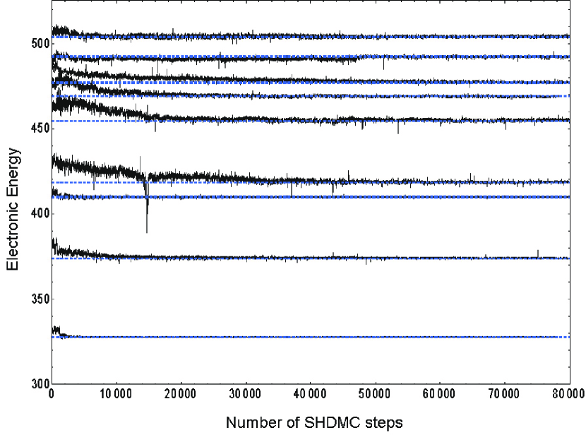
Figure 1: (Color online) Self-healed DMC run obtained for successive eigenstates belonging to the $A_{1}$ (trivial) irreducible representation of the group $D_{4}$ in the singlet state. Black lines denote the average value of the local energy. The horizontal blue dashed lines mark the energy of the corresponding excitation in the full CI calculation.

Figure 1 shows the results of successive SHDMC runs for the singlet ground state and the next $8$ excitations that belong to the same symmetry (total spin $S=0$, and irreducible representation $A_{1}$ of the group $D_{4}$). The SHDMC calculations were done using $N_{c}=200$ walkers with a sub-block length $k=50$, a time step $\delta\tau=0.0002$, units $\delta\tau^{\prime}=0.002$ (for the ground state $\delta\tau^{\prime}=0$ ) and, $\beta=1$ in Eq. (21).

The lines in Fig. 1 join the values obtained for the weighted average of the local energy $E_{L}({\bf R})$ for each time step. The horizontal dashed lines mark the energy of the nearly analytical result obtained with full CI. The agreement between SHDMC and full CI is extremely good. As higher energy eigenstates are calculated however, and the number of nodal pockets and nodal surfaces increases, time step errors start to play a dominant role. In particular, for the $9^{th}$ excitation (not shown) $\delta\tau$ must be reduced.

The occasional peaks (or drops) observable in the data are correlated with the update of $\Psi_{T}({\bf R})$, and their reduction also reflects a systematic improvement in the trial wave-function. At the end of each block, the trial wave-function coefficients $\lambda_{n}$ are updated and all weights are reset to 1. They gradually reach equilibrium values when new energies are sampled, completing a sub-block of length $k$. As a result, at the beginning of each block, the energy sampled is the average of the trial wave-function energy, which is often different than the DMC energy sampled thereafter (but it can be smaller or higher for a bad trial wave-function with small $N_{c}$).

One interesting result is that some orthogonality constraints are not required to obtain some excited states. This is the case, for example, of the first excited state calculated with $\beta=1$. This is presumably due to the fact that the number of nodal pockets is different for the excited state and the ground state and the decay path from the first excited state to the ground state is obstructed by the formation of a kink between inequivalent nodal pockets if a value of $\beta\approx 1$ is used. This is also the case for states $6$ and $7$, which were obtained before state 5 despite the fact that they have higher energy.

A similar effect is observed in some triplet excitations. Due to the choice of initial trial wave-function and the kink induced by $\beta=1$, the $3^{rd}$ excitation is found before the $2^{nd}$, and the $5^{th}$ is obtained before the $2^{nd}$ and the $4^{th}$. This interesting effect disappears if $\beta=0$ is chosen.

Table 1 shows the logarithm of the residual projection

$$L_{rp}=\log\left(1-|\langle\Psi_{n}^{CI}|\Psi_{n}\rangle|\right)$$ (23)

of the excited state wave-function $|\Psi_{n}\rangle$ sampled with SHDMC onto the corresponding full CI result $|\Psi_{n}^{CI}\rangle$ as a function of the number of iterations for different eigenstates. The states are ordered as they first appear in the calculation.

In addition, Table 1 compares the values of the eigen-energies obtained with CI and SHDMC. The agreement is very good. In some cases the difference is larger than the error bar. This might signal that small nodal errors remain. Note that there is no upper bound theorem for excited states but for the ground state within an abelian irreducible representation.foulkes99

Table 1: Values obtained for $L_{rp}$ [see Eq. (23) ] for a total of (a) $4\times 10^{4}$ (b) $8\times 10^{4}$ and (c) $12\times 10^{4}$ DMC steps and corresponding eigen-energies for two electrons in a square box with a model interaction. The logarithm of the residual projection $L_{rp}$ of the SHDMC wave-function with the corresponding full result CI is given for different eigenstates belonging to the same symmetry of the ground state as a function of the number of steps used to sample the wave-function. The states are included in the order they were obtained.

State	Spin	Rep.	$L_{rp}$	$L_{rp}$	$L_{rp}$	CI	SHDMC
			a	b	c	Energy	Energy
0	S	A1	-14.84	-15.05		328.088	328.089	(2)
1	S	A1	-6.80	-8.85		374.106	374.103	(6)
2	S	A1	-7.23	-8.69		409.960	409.954	(3)
3	S	A1	-4.42	-6.07		418.508	418.66	(2)
4	S	A1	-3.65	-5.01		454.630	454.84	(2)
6	S	A1	-.–	-4.85	-6.22	477.019	477.100	(5)
7	S	A1	-3.90	-5.26		492.216	491.98	(1)
5	S	A1	-5.60	-6.17		468.854	468.845	(13)
8	S	A1	-5.09	-6.49		503.805	503.92	(1)
0	T	E	-8.49	-8.71		342.137	342.191	(5)
1	T	E	-4.37	-4.35		385.908	387.80	(1)
3	T	E	-3.06	-3.35		422.670	423.60	(2)
5	T	E	-4.04	-5.48		438.791	438.70	(1)
2	T	E	-2.31	-2.31		411.887	416.07	(1)

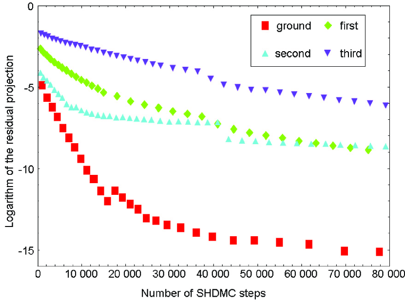
Figure 2: (Color Online) Logarithm of the residual projection [see Eq. (23)] for the ground (square), first (diamond), second (up triangle) and third (down triangle) eigenstates with $A_{1}$ symmetry and S=0.

Figure 2 shows $L_{rp}$ at the end of each block for the ground state and low-lying excitations of the system as a function of the total number of SHDMC steps. The calculations were done by first running $\sim\!40\,000$ SHDMC steps for each eigenstate before starting the calculation of the next. Subsequently, an additional set of $\sim\!40\,000$ SHDMC steps was run, improving the projector $\hat{P}$. The kinks in the data around $\sim~{}40\,000$ are due to the changes in the coefficients of the lower energy states involved in $\hat{P}$ [see Eq. (17)].

One important conclusion of Table 1 and Figure 2 is that errors in the determination of lower energy states calculated earlier only propagate “locally” because of the orthogonality constraints in Eq. (17). This error does not have a strong impact on much higher energy excitations. This is apparently due to the fact that each newly calculated excitation tends to occupy the Hilbert space left by lower excitations due to statistical error. This is clear, for example, for the $5^{th}$ and $8^{th}$ excitations, which have an error much smaller than several excitations calculated earlier (e.g., $3^{rd}$ and $4^{th}$). The error in the $3^{rd}$ and $4^{th}$ excitations is mainly due to mixing among themselves. This result is important because it means that the present method can be used to calculate several higher excitations in spite of the errors in lower energy ones.

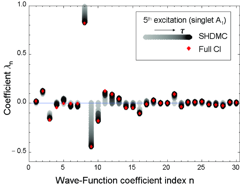
Figure 3: (Color online) Change in the values of the multi-determinant expansion as the DMC self-healing algorithm progresses for the $5^{th}$ excited state of the singlet state of $A_{1}$ symmetry. Light gray colors denote older coefficients, whereas darker ones denote more converged results. The full CI results are highlighted in small red diamonds.

Figure  3 shows the evolution of the values of the coefficients $\lambda_{n}^{\ell}$ of $|\Psi_{T}^{\ell}\rangle$ as a function of the coefficient index $n$ for the $5^{th}$ excited state corresponding to the singlet configuration of the $A_{1}$ representation of the group $D_{4}$. The shade of gray is light for the older (small $\ell$) coefficients and deepens to black for the final results (large $\ell$). The calculation started from a trial wave-function orthogonal to the states calculated before as described above.

The coefficients of the wave-function sampled with SHDMC overlap with the ones obtained with full CI (see Table 1). Similar results are obtained for all the other excited states calculated. An important observation is that the coefficients $\lambda_{n}$ evolve continuously towards the exact solution, which suggests the possibility of accelerated algorithms that extrapolate the values of $\delta\lambda_{n}$.

Some eigenstates are significantly more difficult to calculate than others. This is typically the case for eigenstates with similar eigenvalues (e.g., the $6^{th}$ excitation in the singlet case). A bigger challenge, however, is when $E_{L}({\bf R})$ is ill behaved, for example, the case of the $2^{nd}$, $4^{th}$, and $6^{th}$ excitations of the triplet state. Even the full CI wave-function with 300 basis functions has a large variance for $E_{L}({\bf R})$. In that case the coefficients obtained with SHDMC and CI are different. This is due to the fact that the two methods minimize different things: CI minimizes $\langle~{}\Psi_{n}~{}|(\hat{\mathcal{H}}-E_{n})^{2}|\Psi_{n}\rangle$ on a truncated basis, and SHDMC minimizes $\int E_{L}({\bf R})f({\bf R},\tau){\bf dR}$ with $\langle\Psi_{T}|\hat{P}|\Psi_{T}\rangle=\langle\Psi_{T}|\Psi_{T}\rangle$. Accordingly, the fact that the results are different indicates that neither calculation, CI or SHDMC, is converged with the basis chosen. The $4^{th}$ and $6^{th}$ excitations with E symmetry in the triplet case obtained with SHDMC are a linear combination of the corresponding ones in full CI.

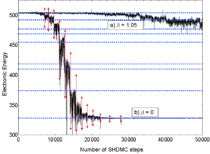
Figure 4: (Color online) Average of the local energy $E_{L}({\bf R})$ as a function to the number of DMC time steps for two SHDMC runs with $\hat{P}=1$ starting from a converged trial wave-function corresponding to the $8^{th}$ singlet excitation of $A_{1}$ symmetry with a) $\beta=1.05$ and b) $\beta=0$ in Eq. (21). The dotted lines mark the beginning of some of the fixed-node DMC blocks of a SHDMC run for the $\beta=0$ case. Same conventions as in Fig. 1.

Figure 4 shows the effect of $\hat{P}$ and $\beta$ [see Eq. (21)] on a SHDMC run. The figure shows the average of the local energy $E_{L}({\bf R})$ for two calculations that start from the final trial wave-function obtained for the $8^{th}$ singlet excitation with $A_{1}$ symmetry (please compare it with Fig. 1). Both calculations were run with the same parameters as in Fig. 1 with two exceptions: i) $\hat{P}=1$ was used, which removes the orthogonality constraints, and ii) one calculation was run with $\beta=1.05$ and the other with $\beta=0$ in Eq. (21). An initial number of blocks $M=20$ was used.

Both calculations depart from the initial configuration. However, the run with $\beta=0$ falls very quickly to the singlet ground state. The calculation with $\beta=1.05$ remains much longer in the vicinity of the $8^{th}$ excitation. This clearly shows the stabilizing effect unequal energy references on excited states. Since presumably the $8^{th}$ excitation is not the minimum of its nodal topology, it finally drifts away. For the $\beta=1.05$ case with $\delta\tau=0.0002$, the algorithm becomes numerically unstable to noise after the $\sim\!50],000$ time step because the variance in the distribution of weights of the walkers increases and the statistics is dominated by a reduced number of walkers.

In contrast, the first excitation does not drift with $\beta\simeq 1$ and $\hat{P}=1$ (not shown).

V.1 Coulomb interaction results and discussion

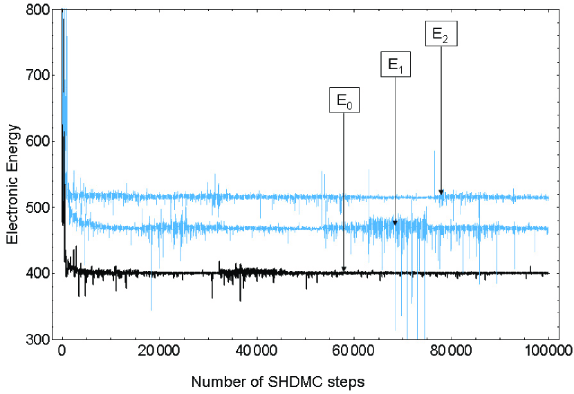
Figure 5: (Color online) Average of the local energy $E_{L}({\bf R})$ of 200 walkers as the SHDMC algorithm converges to the ground, first and second eigenstates with $A_{1}$ symmetry and S=0 of two electrons with Coulomb interactions in a square box.

The use of a simplified electron-electron interaction facilitates the CI calculations and the validation of the optimization method. However, it is also important to test the convergence and stability of the method with a realistic Coulomb interaction as in the case of the ground state. keystone

The results shown in this section have an interaction potential of the formunits $V({\bf r},{\bf r^{\prime}})=20\pi^{2}/|{\bf r-r\prime}|$ as in Ref. keystone, . To mimic the difficulties that the algorithm would have to overcome in larger or more realistic systems, the Jastrow term is not included, i.e. $J=0$. Most SHDMC parameters are the same as in the model interaction case. All calculations with Coulomb interactions were run with $\beta=0$, the initial number of sub-blocks $M=6$, and the time step reduced to $\delta\tau=0.0001$. The initial trial wave-functions were selected with the criteria used for the model case.

Figure 5 shows the average of the local energy $E_{L}({\bf R})$ obtained for the ground state and the first two excitations with the same symmetry (singlet $A_{1}$). The results are qualitatively similar to those obtained with the model potential. It is evident from the data that the variance of $E_{L}({\bf R})$ and its average are reduced as the wave-function is optimized. Occasionally, $E_{L}({\bf R})$ might rise when $\hat{P}$ is updated (improving the description of lower energy states).

The energy of the singlet ground state is 400.749 $\pm$ 0.013, which is only slightly smaller than the lowest triplet energykeystone 402.718 $\pm$ 0.008 with symmetry $E$. These energies are very close because of the dominance of the Coulomb repulsion as compared to the kinetic energy, which forces the particles to be well separated and therefore the cost of a node in the triplet state is small. This result is consistent with the choice of parameters that sets the system in the highly correlated regime. The energies obtained for the first and second excitations areunits $468.56\pm 0.09$ and $515.50\pm 0.08$ respectively.

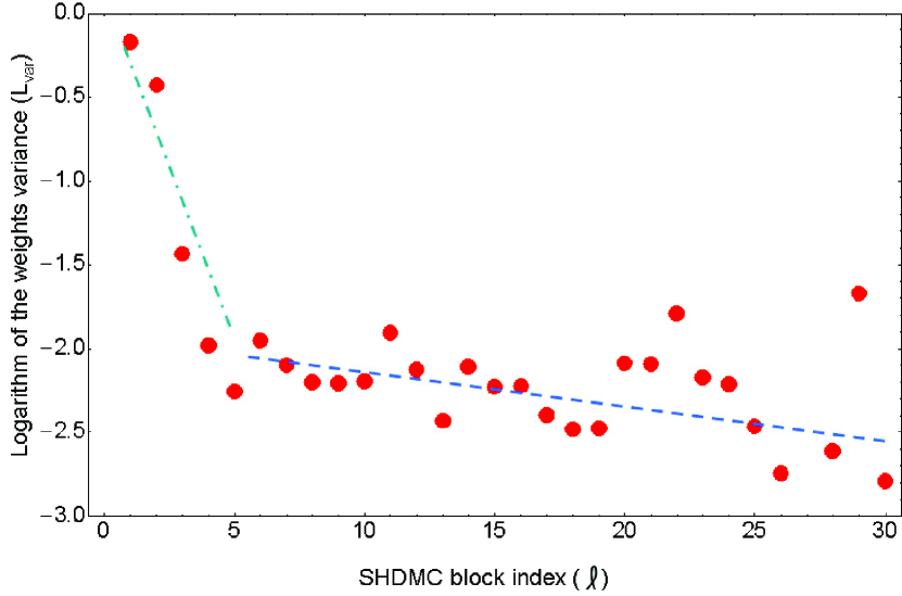
Figure 6: (Color online) Logarithm of the variance of the weights of the walkers distribution as a function of the SHDMC block index $\ell$ for the $2^{nd}$ excitation with $A^{1}$ symmetry with Coulomb interaction (see Fig. 5). The lines are visual guides.

While Figs. 1 and 5 are qualitatively similar, the results shown in Fig. 1 are more convincing since they are directly compared with full CI calculations and they are less noisy, as noted by one referee. When the model interaction potential is replaced by a Coulomb interaction, full CI calculations are still possible, but they involve the numerical calculation of $16471$ integrals with Coulomb singularities. CI calculations are typically done using a Gaussian basis, dupuis which limits the impact of the matrix element integrals of these singularities. However, as the size of the system increases, CI calculations become too expansible numerically. Accordingly, self-reliant methods to validate the quality of the SHDMC wave-functions must be developed.

As noted earlier, in a fixed population scheme, the weights contain all the difference between $f({\bf R},\tau)$ and $|\Psi_{T}({\bf R})|^{2}$ . Since $f({\bf R},\tau)$ and $|\Psi_{T}({\bf R})|^{2}$ should be equal if $\Psi_{T}({\bf R})$ is an eigenstate, the variance of the weights can be used to measure the quality of the wave-function. Figure 6 shows the evolution of the logarithm of the variance $L_{var}$ of the weights of the walkers $W_{i}^{j}(k)$ [see Eq. (3)] as a function of the SHDMC block index $\ell$. $L_{var}$ is evaluated as

$$L_{var}=\log{\sqrt{\frac{1}{N_{c}}\sum_{i,j}(W_{i}^{kj}(k)-1)^{2}}}\;.$$ (24)

By using a linear order expansion in $\delta\tau$ in Eq. (3) and using Eq. (4), it is straightforward to relate Eq. (24) to the variance of $E_{i}^{j}(k)$. The latter is an average of $E_{L}({\bf R})$. A common measure of the quality of the ground state wave-function is the variance of $E_{L}({\bf R})$.

The results shown in Fig. 6 correspond to the $2^{nd}$ singlet excitation with $A_{1}$ symmetry (see Fig. 5). Similar results are obtained for the ground state and the first excitation (not shown). The error bar in $L_{var}$ is smaller than the size of the symbols. The fluctuations in $L_{var}$ result from the random fluctuations of the coefficients $\lambda_{n}$ that are obtained statistically. Note that in spite of the noise, a clear trend shows the improvement of the quality of the wave-function and $E_{T}$ as the SHDMC algorithm progresses. However, these improvements are not uniform, which is reflected by the oscillations in $L_{var}$ in Fig. 6 and in the amplitude of $E_{L}({\bf R})$ in Fig. 5. A careful user of SHDMC should track $L_{var}$ and use the best quality wave-function to calculate energies and $\hat{P}$.

VI Summary

An algorithm to obtain the approximate nodes, wave-functions, and energies of arbitrary low-energy eigenstates of many-body Hamiltonians has been presented. This algorithm is a generalization of the “simple” self-healing diffusion Monte Carlo method developed for the calculation of the ground state of fermionic systems,keystone which in turn is built upon the standard DMC method. ceperley80

At least in the case of the tested system, wave-functions and energies that continuously approach fully converged configuration interaction calculations can be obtained depending only on the computational time. The wave-function, in turn, allows the calculation of any observable.

It is found that some special eigenstates, presumably the minimum energy eigenstate for a given nodal topology, can be obtained without calculating the lower excitations by artificially generating a kink in the propagated function using unequal energy references in different nodal pockets.

The present method can be implemented easily in existing codes. Ongoing tests on the ground state methodkeystone in larger systems give serious hopefn:tests that the current generalization will also be useful.

While there are methods to obtain the excitation spectra of a many-body Hamiltonian in a variational Monte Carlo context kent98 ; umrigar07 they require obtaining the Hamiltonian and the overlap matrix elements. This requirement would present a challenge for very large systems. SHDMC is a complementary technique that could potentially scale better for larger sizes. The evaluation and storage of the matrix elements of $\hat{\mathcal{H}}$ is not required. The number of quantities sampled [the projectors $\xi_{n}({\bf R})$, Eq. (14)] is equal to the number of basis functions $n_{b}$. In contrast, energy minimization methods or configuration interaction (CI) require the evaluation of $n_{b}^{2}$ matrix elements. In addition, the solution of a generalized eigenvalue problem with statistical noise is avoided. This can be an advantage in very large systems since algorithms for eigenvalue problems are difficult to scale to take maximum advantage of large supercomputers. In contrast, the sampling of a large number of determinants can be trivially distributed on different processors. Moreover, recent advances in determinant evaluation could facilitate sampling a very large number of projectors $\xi_{n}({\bf R})$. nukala09

An apparent disadvantage of SHDMC is that the method is recursive. This disadvantage is partially removed since i) the number of blocks $M$ used to collect data is increased only if necessary to improve the wave-function significantly, fn:changes ii) and, the propagation to large imaginary times is avoided by using precisely this recursive approach that accumulates the propagation in successive blocks. In addition, a small value of $k\;\delta\tau$ limits large fluctuations in the weights, which recently have been claimed to cause an exponential cost in the convergence of DMC results. nemec09

The dominant cost of the present algorithm to obtain the wave-functions and their nodes scales as $N_{e}^{3}\times n_{max}\times n_{b}\times n_{st}$, with $n_{max}$ being the number of excited states, $n_{b}$ the number of projectors $\xi_{n}({\bf R})$ sampled, and $n_{st}$ the total number of SHDMC steps. Of course, the error and the cost depend on the quality of the method used to construct $\Phi_{n}({\bf R})$ and the quality of the initial trial wave-functions. Systematic errors decrease when $n_{b}$ is large, and the statistical error decreases when $n_{st}$ increases. For a fixed absolute error, $n_{b}$ is expected to increase exponentially with the number of electrons $N_{e}$. keystone

Note that in order to describe an arbitrary wave-function of a system with $N_{e}$ electrons and a typical size $L$ in $D>1$ dimensions with a resolution $R_{s}$, one needs approximately $(L/R_{s})^{(D\;N_{e})}$ basis functions. The nodal surface alone requires  $(L/R_{s})^{(D\;N_{e}-1)}$ degrees of freedom. Therefore, finding an algorithm to obtain the nodes $S_{n}({\bf R})$ of any eigenstate $n$ with an arbitrary interaction in a time polynomial in $N_{e}$ is potentially a “Philosopher’s Stone” quest. However, if exponential factors actually control the accuracy of the DMC approach, as claimed, nemec09 just a rock solid method to find the nodes which simultaneously improves the wave-function (reducing the population fluctuations) could be considered a satisfactory solution. The presented work could be the basis of such a method.

In ongoing work, SHDMC methods are being developed and tested in larger systems.

References

- (1) P. Hohenberg and W. Kohn, Phys. Rev. 136, B864 (1964).
- (2) W. Kohn and L. J. Sham, Phys. Rev. 140, A1133 (1965).
- (3) L. Hedin, Phys. Rev. 139, A796 (1965).
- (4) D. M. Ceperley and B. J. Alder, Phys. Rev. Lett. 45, 566 (1980).
- (5) W. M. C. Foulkes, R. Q. Hood, and R. J. Needs, Phys. Rev. B 60, 4558 (1999).
- (6) J. B. Anderson, Int. J. Quantum Chem. 15, 109 (1979).
- (7) P. J. Reynolds, D. M. Ceperley, B. J. Alder, and W. A. Lester, J. Chem. Phys. 77, 5593 (1982).
- (8) F. A. Reboredo, R. Q. Hood, and P. R. C. Kent, Phys. Rev. B 79, 195117 (2009)
- (9) D. M. Ceperley, J. Stat. Phys. 63, 1237 (1991).
- (10) F. A. Reboredo and P. R. C. Kent, Phys. Rev. B 77, 245110 (2008).
- (11) Understanding sections I, II, III, V and VI of Ref. keystone, is required before reading this article.
- (12) The energy unit is .
- (13) C. J. Umrigar, M. P. Nightingale, and K. J. Runge, J. Chem. Phys. 99, 2865 (1993).
- (14) Note that the limit is taken after the amplitude of the potential tends to . Thus, this potential does not have the form, and every eigenstate of must be zero at .
- (15) The Jastrow factor does not change the nodes but accelerates convergence and improves the algorithm’s numerical stability.
- (16) The ground state is formally obtained byapplying the evolution operator to a trial wave-function in the limit .
- (17) S. Vitiello, K. Runge, and M. H. Kalos, Phys. Rev. Lett. 60, 1970 (1988).
- (18) R. Bianchi, D. Bressanini, P. Cremaschi, M. Mella, and G. Morosi, J. Chem. Phys. 98, 7204 (1993).
- (19) R. Bianchi, D. Bressanini, P. Cremaschi, M. Mella, and G. Morosi, Int. J. Quant. Chem. 57, 321 (1996).
- (20) B. L. Hammond, W. A. Lester, Jr., and P. J. Reynolds Monte Carlo Methods in Ab Initio Quantum Chemistry (World Scientific, Singapore-New Jersey-London-Hong Kong, 1994).
- (21) D. M. Ceperley and B. Bernu, J. Chem. Phys. 89, 6316 (1988).
- (22) R. N. Barnett, R. P. Reynolds, and W. A. Lester, J. Chem. Phys. 96, 2141 (1991).
- (23) D. Blume, M. Lewerenz, P. Niyaz, and K. B. Whaley, Phys. Rev. E 55, 3664 (1997).
- (24) W. D. da Silva and P. H. Acioli, J. Chem. Phys. 114, 9720 (2001).
- (25) M. P. Nightingale and V. Melik-Alaverdian, Phys. Rev. Lett. 87, 043401 (2001).
- (26) A. Lüchow, D. Neuhauser, J. Ka, R. Baer, J. Chen, and V. A. Mandelshtam, J. Phys. Chem. A 107, 7175 (2003).
- (27) F. Schautz, F. Buda, and C. Filippi, J. Chem. Phys. 121, 5836 (2004).
- (28) C. J. Umrigar, J. Toulouse, C. Filippi, S. Sorella, and R. G. Hennig, Phys. Rev. Lett. 98, 110201 (2007).
- (29) W. Purwanto, S. Zhang, and H. Krakauer, J. Chem. Phys. 130, 094107 (2009).
- (30) All symmetries of must be considered, which includes space group symmetries, spin, and particle permutations.
- (31) C. Umrigar, private communication. A description of the benefits of his suggested improvement for the ground state will be published elsewhere.
- (32) If the change in the wave-function coefficients is dominated by random noise, the scalar product between the old and the new can be negative and is multiplied by a factor larger than 1.
- (33) M. Dupuis, and J. A. Montgomery, J. Comput. Chem. 14, 1347-1363 (1993).
- (34) P. K. V. V. Nukala and P. R. C. Kent, J. Chem. Phys. 130, 204105 (2009).
- (35) A SrLi dimer with electrons has been compared with energy minimization calculations.umrigar07 We have also a proof of principle for C (78 electrons and 700 determinants).
- (36) P. R. C. Kent, R. Q. Hood, M. D. Towler, R. J. Needs, and G. Rajagopal, Phys. Rev. B. 57, 15293 (1998).
- (37) N. Nemec, in http://arxiv.org/abs/0906.0501