The Sizes of the X-ray and Optical Emission Regions of RXJ 1131–1231
Abstract
We use gravitational microlensing of the four images of the quasar RXJ 1131–1231 to measure the sizes of the optical and X-ray emission regions of the quasar. The (face-on) scale length of the optical disk at rest frame 400nm is cm, while the half-light radius of the rest frame 0.3–17 keV X-ray emission is cm. The formal uncertainties are factors of and , respectively. With the exception of the lower limit on the X-ray size, the results are very stable against any changes in the priors used in the analysis. Based on the H line-width, we estimate that the black hole mass is , which corresponds to a gravitational radius of cm. Thus, the X-ray emission is emerging on scales of and the 400 nm emission on scales of . A standard thin disk of this size should be significantly brighter than observed. Possible solutions are to have a flatter temperature profile or to scatter a large fraction of the optical flux on larger scales after it is emitted. While our calculations were not optimized to constrain the dark matter fraction in the lens galaxy, dark matter dominated models are favored. With well-sampled optical and X-ray light curves over a broad range of frequencies there will be no difficulty in extending our analysis to completely map the structure of the accretion disk as a function of wavelength.
Subject headings:
accretion – accretion disks – black hole physics – gravitational lensing—quasars: individual (RXJ 1131–1231)1. Introduction
A significant problem for theoretical studies of quasars is that we cannot spatially resolve their emission regions to test models (e.g. Blaes 2004). For example, in this paper we study the gravitational lens RXJ 1231–1131 (RXJ1131 hereafter), where we observe four images of a quasar lensed by a elliptical galaxy (Sluse et al. 2003). Based on the H line-width from Sluse et al. (2003), and a magnification corrected estimate of the continuum luminosity, we estimate111Using the Bentz et al. (2006) mass normalizations. For the Kaspi et al. (2005) normalization we obtain , which is consistent with the earlier estimate of Peng et al. (2006) of also using the Kaspi et al. (2005) normalizations. We use the Peng et al. (2006) masses in Morgan et al. (2009) because we lacked spectra for the full sample of objects. that the black hole mass, , is . This corresponds to a gravitational radius of
| (1) |
that subtends only micro-arcseconds.
Gravity, however, has provided us with a natural telescope for studying the structure of quasars through the microlensing produced by stars in the lens galaxy (see the review by Wambsganss 2006). Microlensing has a natural outer length scale corresponding to the Einstein radius of the stars,
| (2) |
where is the mean mass of the stars, and the distances , and are the angular diameter distances between the observer, lens and source. The microlenses also generate caustic lines on which the magnification diverges, which means that our gravitational telescope can, for all practical purposes, resolve arbitrarily small sources. The size of the source is encoded in the amplitude of the microlensing variability as the source, lens, and observer move relative to the caustic patterns – big sources have smaller variability amplitudes than small sources. The technique can be applied to any emission arising from scales more compact than a few .
If we model the accretion disk by a thermally radiating thin disk with a temperature profile of (Shakura & Sunyaev 1973)222In our present analysis we can neglect the drop in temperature and emission near the inner edge of the accretion disk as it has little effect on the results., we can measure the scale defined by the point where the photon energy equals the disk temperature, , by two routes other than microlensing. First, we can estimate it from the observed flux at some wavelength. For example, at I-band the radius is
| (3) |
where is the Hubble radius, and is the inclination angle of the disk. Based on HST observations (Sluse et al. 2006; Kozłowski et al. 2009), we estimate that the magnification-corrected flux is mag (m), which corresponds to an R-band (400 nm in the quasar rest frame) size of cm or about . The flux size depends on the mean magnification of the images as , which can introduce a systematic uncertainty into this size estimate. Second, thin disk theory predicts that
which implies an R-band disk size cm () if the disk is radiating at the Eddington limit with an efficiency of . Note that these two size estimates can be reconciled only if , corresponding to a sub-Eddington accretion rate, an overestimated black hole mass, or a problem in the disk model since there is no evidence for the 1–2 mags of extinction in the lens galaxy that would be needed raise the flux size up to that from thin disk theory (Eqn. 1). Adding the inner disk edge or using a simple relativistic disk model (Novikov & Thorne 1973, Page & Thorne 1974) changes this problem little.
The expected size of the X-ray emitting regions is more problematic because there is no comparably simple model for our theoretical expectations. There is a general consensus that the X-ray continuum emission is due to unsaturated inverse Compton scattering of soft photons by hot electrons in a corona surrounding the inner parts of the accretion disk (see the review by Reynolds & Nowak 2003), but the extent and geometrical configuration of the X-ray emission region is an open question. The X-ray continuum from the corona illuminates the disk to produce Fe K emission lines, whose broad widths indicate that they are generated close to the inner edge of the accretion disk (e.g. Fabian et al. 2005).
While there were a number of early attempts at estimating accretion disk sizes using microlensing (e.g. Wambsganss, Schneider & Paczyński 1990, Rauch & Blandford 1991, Wyithe et al. 2000b, Wambsganss et al. 2000, Goicoechea et al. 2003), it is only in the last few years that it has become possible to make large numbers of microlensing size estimates. In particular, Pooley et al. (2007) argue that the optical sizes estimated from microlensing must be considerably larger than the optical “flux” sizes of Eqn. 3. This was confirmed by Morgan et al. (2009) in a more detailed analysis that also found that the optical sizes agree better with the thin disk size estimate (Eqn. 1) than the flux size and have a scaling with black hole mass consistent with the scaling for Eddington-limited thin disks.
Recent studies have started to examine the temperature dependence of disks through the scaling of disk size with wavelength (Anguita et al. 2008, Poindexter et al. 2008, Agol et al. 2009, Bate et al. 2009, Floyd et al. 2009, Mosquera et al. 2009). Studies of the microlensing of the X-ray emission are more limited, but indicate that the X-ray emission is much more compact than the optical (Dai et al. 2003, Pooley et al. 2006, 2007, Kochanek et al. 2006, Morgan et al. 2008, Chartas et al. 2009), tracking much closer to the inner edge of the accretion disk. In this paper we estimate the sizes of the optical and X-ray emission regions of RXJ1131 using microlensing. In §2 we describe the data and the analysis method. In §3 we discuss the results, their implications and directions for further research. We use an flat cosmological model with km s-1 Mpc-1 and .
2. Data and Analysis
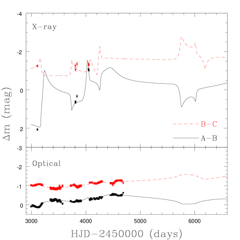
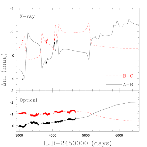
The optical data consist of the five seasons of R-band monitoring data described in Kozłowski et al. (2009). For our present analysis we simply shifted the light curves by their measured time delays (Kozłowski et al. 2009). The X-ray data, all ACIS observations from the Chandra Observatory, consist of the epoch presented by Blackburne et al. (2006) plus the 5 epochs presented in Chartas et al. (2009). Each of the Chartas et al. (2009) epochs consisted of a 5 ksec observation using ACIS-S3 in 1/8 sub-array mode from which we measure the 0.2-10 keV flux. Chartas et al. (2009) also reanalyzed the Blackburne et al. (2006) data to properly correct for the “pile-up” effect. We do not use the X-ray fluxes of image D in our analysis because we cannot presently be certain its flux ratios relative to A–C are unaffected by source variability given the roughly month time delay between D and A–C (Kozłowski et al. 2009). As we can see from Fig. 5, the X-ray source must be more compact than the optical source because the X-ray flux ratios are dramatically more variable.
A full description of our microlensing analysis method is presented in Kochanek (2004) and Kochanek et al. (2006). In essence, we create the microlensing magnification patterns we would see for a broad range of lens models and source sizes, then randomly generate light curves to find ones that fit the data well. We then use Bayes’ theorem to combine the results for the individual trials to infer probability distributions for physically interesting variables including the uncertainties created by all the other variables.
We fit the lens as in Kozłowski et al. (2009), modeling it as a de Vaucouleurs model for the stellar distribution embedded in an NFW halo. We consider a sequence of models described by , the fraction of mass in the stellar component relative to a constant mass-to-light ratio model with and no halo. We include models with to in equal steps, and the time delay measurements favor . These lead to the values for the convergence , shear and fraction of the convergence in stars reported in Table. 1.
The stars creating the microlensing magnification were drawn from a power law mass function with a ratio of 50 between the minimum and maximum masses that roughly matches the Galactic disk mass function of Gould (2000). We know from previous theoretical studies that the choice of the mass function will have little effect on our conclusions given the other sources of uncertainty (e.g. Paczyński 1986, Wyithe et al. 2000a). The mean mass is left as a variable with a uniform prior over the mass range .
For each model we generated 8 random realizations of the star fields near each image. The magnification patterns had an outer scale of cm and a pixel scale of , so we should be able to model sources as compact as the inner edge of the accretion disk. We modeled the relative velocities as in Kochanek (2004), where for RXJ1131 the projection of the CMB dipole velocity (Kogut et al. 1993) on the lens plane is 47 km/s, the lens velocity dispersion estimated from the Einstein radius is km/s, and the estimated rms peculiar velocities of the lens and source galaxies are and km/s respectively.
The source model for both the optical and X-ray sources is a face-on disk with a temperature profile radiating as a black body (Shakura & Sunyaev 1973), so the surface brightness profile of the disk is
| (5) |
with the single parameter being the scale length . While it is true that this profile lacks the central drop in emissivity and that it is not a physical model for the non-thermal X-ray emission, the microlensing analysis is not sensitive to these details. The estimate of the half-light radius () is essentially independent of the assumed profile (Kochanek 2004, Mortonsen, Schechter & Wambsganss 2005). We used a logarithmic grid of trial source sizes for the X-ray and optical sources with a spacing of dex.
We do, however, allow for the possibility that fraction to of the optical emission is generated on scales much larger than the disk and is unaffected by microlensing. Such large scale emission could have two physical origins. First, the optical continuum can be significantly contaminated by emission lines, both the obvious broad lines and the less obvious Fe and Balmer pseudo-continuum emission ( of the emission in some Seyferts, Maoz et al. 1993), that are believed to be produced on much larger scales than the disk. For our R-band light curves, there are no strong emission lines in the filter band pass, but the blue edge of the Balmer continuum emission (Å) does lie inside the band pass (roughly –Å). Second, even if the observed photons were generated by the accretion disk, a fraction could be scattered on much larger scales, leading to an effectively larger source. These two possibilities are not equivalent, as the line emission is due to reprocessing of shorter wavelength UV photons rather than the observed R-band continuum.
A basic problem for any microlensing analysis is the degree to which the “macro” lens model correctly sets the average magnifications. Each light curve, is defined by the source light curve , the macro model magnification , the microlensing magnification and a possible offset . These offsets can be non-zero due to problems in the macro model or the presence of unrecognized substructures that perturb the magnifications (e.g. Kochanek & Dalal 2004), because of differential absorption due to dust or gas in the lens galaxy (e.g. Falco et al. 1999, Dai & Kochanek 2009), or due to contamination of the light curves by flux from the quasar host or lens galaxy. For the latter two possibilities, the offsets would differ between the optical and X-ray light curves. Given a sufficiently long light curve, the offsets can be determined from the data, but they are poorly constrained until the light curve is a good statistical sampling of the magnification pattern. We will consider four treatments of this problem to ensure that such systematic problems do not affect our results. The basic division we will refer to as Cases I and II. In Case I we allow the magnification offsets to float independently for the two bands constrained by a term in the log likelihood with mag. In Case II we allow them to float, but use the same offsets for both the optical and X-ray light curves. These are weak constraints, so the resulting distributions for the offsets are broad. To make sure we are not allowing too much freedom, we also examined limiting the range of the offsets to mag in Cases I’ and II’.
The advantage of the less constrained strategies is that they are robust against the systematic errors that can plague the absolute magnifications of the images. It is certainly true that analyses using only the “DC” flux ratios (e.g. Pooley et al. 2006, 2007, Bate et al. 2009, Floyd et al. 2009) require less data than our “AC” approach, but they can also lead to conclusions dominated by these systematic errors. The “AC” approach also has the advantage that including the effects of the velocities allows us to estimate source sizes in centimeters without simply assuming a mean mass . However, when we use loose priors on the DC flux ratios, we lose significant information on the locations of the images relative to the magnified and demagnified regions of the patterns. As such, it is a conservative approach. We consider all four offset treatments in order to explore their consequences on estimates of the source size and the amount of dark matter in the lens.
We used 8 statistical realizations of the microlensing magnification patterns for each of the 10 stellar surface densities () and for 5 un-microlensed fractions of optical light (). We modeled the data sequentially, making trials for each optical source size and case, and then fitting each trial that was a reasonable statistical fit to the optical data to the X-ray data for each of the X-ray source sizes. In this second step we considered both the case where the X-ray and optical share the same intrinsic flux ratios and where they are allowed to differ.


3. Results and Discussion
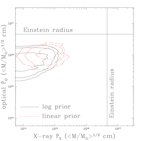
Fig. 1 shows the main result for the estimated size of the X-ray and optical emission regions. These combine all four treatments of the magnification offsets. Also note that in order to preserve the meaning of size ratios in Fig. 1, we used the scale of a face-on disk for both. Physically, the X-ray emission is better characterized by its half light radius, . The scale length of the thin disk also scales as if not viewed face on. We show the results for two different priors on the disk sizes, a logarithmic () and a uniform () prior, and this has minor effects for the optical estimate and significant effects for the X-ray estimate. For the logarithmic prior we formally find that the (face on) optical disk scale length is () and that the X-ray half-light radius is (). These estimates use both the prior on the velocities and a uniform prior for the mass over the range . We will focus on results including this mass prior, but note that if we make no assumption about , the sizes change little. With only the velocity priors we find () and (). The source sizes become a little bit smaller, but the net effect is very modest for the reason outlined in Kochanek (2004).333In Einstein units, one can achieve the observed variability using either a large source moving rapidly or a small source moving slowly, with a degeneracy of roughly . We always impose a prior on the physical velocity , so the physical source size is essentially independent of given a prior on the velocity.
The X-ray size is more sensitive to the priors because the convergence of the probability distributions for small sources is poor when the light curve is sparsely sampled. Fig. 2 shows likelihoods for the source size in the Einstein units used for the basic calculations, and we see that they converge for small X-ray sizes when we use a linear prior but not for a logarithmic prior. The problem is not due to the pixel scale of the maps, but due to the lack of a well-sampled peak in the X-ray data. Very small source sizes are constrained by the magnification peaks observed during a caustic crossing. If the light curve only samples up to some minimum physical distance from a caustic crossing, then it will constrain sources sizes significantly smaller than that distance poorly and the likelihood function will flatten for small source sizes. A logarithmic size prior then favors these small scales compared to a linear prior, leading to significant differences. Thus, our lower limits on the size of the X-ray emission are at a minimum prior dependent. More conservatively, the results could be interpreted as providing only an upper bound on the size of the X-ray emitting region.
Fig. 3 shows how the sizes depend on the priors, the treatment of the magnification offsets and the fraction of the optical emission that is unaffected by microlensing. The X-ray size is affected only by the choice of the size prior. The optical size is only affected by . There are no significant differences between the results for the four magnification offset cases. In order to produce the same optical variability with a larger fraction , we must shrink the disk scale length . Mortonson et al. (2005) argue that the effects of microlensing are largely determined by the half-light radius of the source, which is in the limit that . As we increase , the disk scale length shrinks roughly by the amount needed to keep the half light radius constant, with when . Note, however, that the scaling for this particular model will break down when .
The larger values of are favored, with likelihood ratios of , , , and for , , , and respectively. These differences are only marginally significant, but they are in the sense of favoring (effectively) a flatter temperature profile. A flatter temperature profile can help to reconcile the differences between the larger microlensing and thin disk theory sizes as compared to the smaller flux sizes. Such flatter temperature profiles are generally consistent with the studies of the optical/infrared wavelength dependence of microlensing (Anguita et al. 2008, Eigenbrod et al. 2008, Poindexter et al. 2008, Mosquera et al. 2009, Bate et al. 2009), but are not required. The one exception is Floyd et al. (2009), who find a limit requiring a steeper temperature profile. Some of this information is also present in the overall spectral energy distribution, and it is a long standing problem that the spectra of quasars do not match the predictions of thin disk theory (see Koratkar & Blaes 1999, Gaskell 2008).
Whether increasing helps to resolve the size discrepancies depends on the physical model for the contamination. Line emission is reprocessed shorter wavelength emission, so as we increase we are also reducing the fraction of the observed emission due to the disk and the flux size also shrinks as . If, however, we view it as scattering fraction of the continuum emission on some large scale, then the flux size estimate is unchanged and the effect helps to reduce the discrepancy. Resolving the discrepancy with would require that most of the optical emission does not reach us directly from the accretion disk.
While the source sizes show little dependence on the treatment of the magnification offsets, estimates of the amount of dark matter in the lens are sensitive to how strongly we constrain the models to match the observed macro model flux ratios, as illustrated in Fig. 4. By leaving the offsets relatively free, so as to conservatively estimate the source sizes, we have not optimized the calculation for probing dark matter. The Case I and II models, where we very loosely constrain the allowed magnification offsets, marginally favor models with . The Case I’ and II’ models, where we only accept small offsets, favor the same dark matter dominated model more strongly. This range for is also that favored by the time delays measurements from Kozłowski et al. (2009). Note, however, that we are not in the “lagoon and caldera” regime for the microlensing patterns noted by Schechter & Wambsganss (2002) because of the very high magnifications ( for image A at low rather than ).
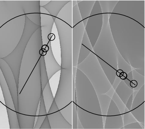
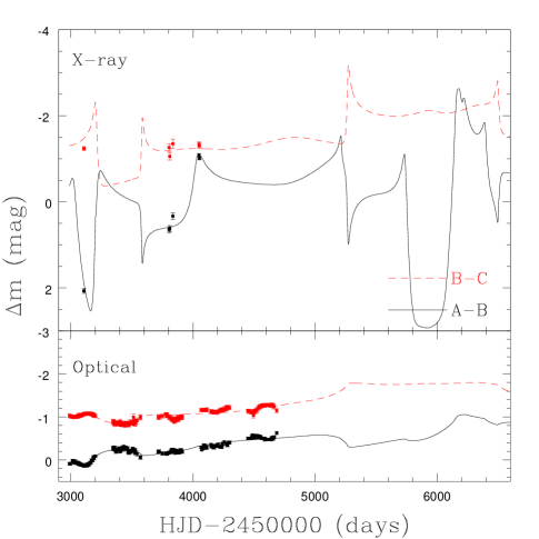
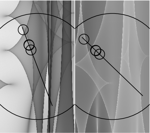
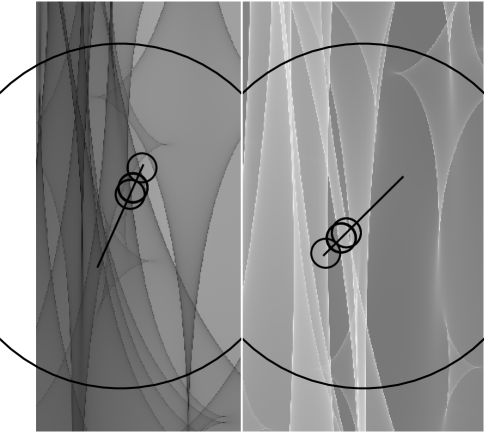
Figs. 5-7 show several examples of model light curves that fit the data reasonably well. These were also selected to have velocities consistent with masses of order -. The solutions are not unique, but they illustrate how simple changes in the source size dramatically alter the amplitude of the variability. A common theme to the solutions is that the A and B images are generally required to lie in “active” regions of the patterns in order to produce such large changes in the X-ray fluxes. This means that we can expect the dramatic variability observed in this system to continue for an extended period of time (– years). It is also interesting to note that significant changes in the optical fluxes are also likely. The larger optical source size washes out the effects of the closely spaced caustics that help to drive the X-ray variability. But the overall changes between the high magnification ridges and the demagnified valleys are still significant, and we should see overall changes in the optical fluxes several times those observed to date.
The implications of these results for theoretical models are mixed. The size of the disk is grossly similar to that expected from thin disk theory, and as we have summarized in Morgan et al. (2009), we find disk sizes that scale with black hole mass and optical wavelength roughly as expected (Eqn. 1). We also find that the X-ray emission arises from significantly closer to the expected inner edge of the accretion disk than the optical emission, as we might expect for a hot corona. The optical size is broadly consistent with the expectations for an Eddington luminosity black hole with a mass estimated from the emission line widths (Eqn. 1). But the size is inconsistent with that expected for a thermally radiating disk with the observed magnitude (Eqn. 3). This is the discrepancy originally noted by Pooley et al. (2006), which we explore more quantitatively in Morgan et al. (2009).
Should we conclude that the thin disk model is wrong or simply that we have oversimplified the optical radiation transfer? We considered contamination by line emission or scattering of the optical photons, finding that this can modestly reduce the disk size for the range where up to 40% of the optical emission does not come directly from the disk. Our simple emission model neglects the disk atmosphere and heating of the outer disk by radiation from the inner disk, all processes which would tend to make the optical emission region larger than the point where the disk has a temperature matching the photon wavelength without any change in the underlying properties of the disk. Many of these effects are included in recent disk models such as Hubeny et al. (2001) or Li et al. (2005) for disk spectra. We examined face-on models with , yr-1 and a BH spin of using the Hubeny et al. (2001) models to compute our definition of the disk scale (, where ) and the half-light radius (). The scale is the most sensitive to the assumptions, with for m in our simplified disk model but equal to / for black body non-relativistic/relativistic disk models (BB NR/REL) and to / for non-LTE non-relativistic/relativistic models (NLTE NR/REL). The model dependence is much reduced if we compare with the half-light radii ( for the simple model, / for the NLTE NR/REL models, and / for the BB NR/REL models). A flatter temperature profile than would help, since at fixed total flux the half light radius increases. For example if , the flux would be only 20% that of our standard profile for the same half-light radius. Indeed, such a flat temperature profile would also come much closer to matching the observed spectra of quasars (e.g. Koratkar & Blaes 1999, Gaskell 2008) and would be representative of models dominated by irradiation. In general, however, current microlensing results on temperature profiles do not favor such flat profiles even if they generally allow somewhat flatter profiles (e.g. Anguita et al. 2008, Eigenbrod et al. 2008, Poindexter et al. 2008, Mosquera et al. 2009, Bate et al. 2009, Floyd et al. 2009).
The key to disentangling these problems is to expand the measurements over a broad range of wavelengths, so that we can constrain the temperature profile of the disk, and over a broad range of black hole masses and accretion rates. For the particular case of RXJ1131, we have programs to continue the X-ray monitoring of the system and to use HST to monitor the ultraviolet flux ratios of the images. Obtaining a robust lower limit to the size of the X-ray emitting region may require denser sampling of the X-ray light curve. Measuring the mid-infrared flux ratios of the images would be the most important step towards rigorously imposing the relative macro magnifications with no offsets, as these would only be affected by the macro model and any large scale gravitational perturbations (satellites).
References
- Agol et al. (2009) Agol, E., Gogarten, S. M., Gorjian, V., & Kimball, A. 2009, ApJ, 697, 1010
- (2) Anguita, T., Schmidt, R.W., Turner, E.L., Wambsganss, J., Webster, R.L., Loomis, K.A., Long, D., & McMillan, R., 2008, A&A, 480, 327
- (3) Bate, N.F., Floyd, D.J.E., Webster, R.L., & Wyithe, J.S.B., 2008, MNRAS, 391, 1955
- (4) Bentz, M.C., Peterson, B.M., Pogge, R.W., Vestergaarrd, M., Onken, C.A., 2006, ApJ, 644, 133
- (5) Blackburne, J.A., Pooley, D., & Rappaport, S., 2006, ApJ, 640, 569
- (6) Blaes, O.M., 2004, in Les Houches Summer School LXXVIII (Springer: Berlin) 137
- (7) Chartas, G., Kochanek, C.S., Dai, X., Poindexter, S., & Garmire, G., 2009, ApJ, 693, 174
- (8) Dai, X., Chartas, G., Agol, E., Bautz, M.W., & Garmire, G.P., 2003, ApJ, 589, 100
- (9) Dai, X., & Kochanek, C.S., 2009, ApJ, 692, 677
- (10) Eigenbrod, A., Courbin, F., Meylan, G., Agol, E., Anguita, T., Schmidt, R.W., & Wambsganss, J., 2008, A&A, 490, 933
- (11) Fabian, A.C., Miniutti, G., Iwasawa, K., & Ross, R.R., 2005, MNRAS, 361, 795
- (12) Falco, E.E., Impey, C.D., Kochanek, C.S., Lehár, J., McLeod, B.A., Rix, H.-W., Keeton, C.R., Muñoz, J.A. & Peng, C.Y., 1999, ApJ, 523, 617
- (13) Floyd, D.J., Bate, N.F., & Webster, R.L., 2009, MNRAS in press [arXiv:0905.2651]
- (14) Gaskell, C.M., 2008, Revista Mexicana de Astronomia Y Astrofisica Conference Series, 32, 1 [arXiv:0711.2113]
- (15) Goicoechea, L.J., Alcaide, D., Mediavilla, E., Munõz, J.A., 2003, A&A, 397, 517
- Gould (2000) Gould, A. 2000, ApJ, 535, 928
- (17) Hubeny, I., Blaes, O., Krolik, J.H., & Agol, E., 2001, ApJ, 559, 680
- (18) Kaspi, S., Maoz, D., Netzer, H., Peterson, B.M., Vestergaard, M., & Jannuzi, B.T., 2006, ApJ, 629, 61
- (19) Kochanek C.S., 2004, ApJ, 605, 58
- (20) Kochanek, C.S., & Dalal, N., 2004, ApJ, 610, 69
- (21) Kochanek, C.S., Dai, X., Morgan, C., Morgan, N., Poindexter, S., & Chartas, G., 2006, Statistical Challenges in Modern Astronomy IV, 2007, G. J. Babu and E. D. Feigelson (eds.), San Francisco:Astron. Soc. Pacific [astro-ph/0609112]
- (22) Koratkar, A., & Blaes, O., 1999, PASP, 111, 1
- (23) Kozłowski, S., Morgan, N.D., Kochanek, C.S., Poindexter, S., Falco, E.E., & Dai, X., 2009, in preparation
- (24) Kogut, A., et al., 1993, ApJ, 419, 1
- (25) Li, L.-X., Zimmerman, E.R., Narayan, R., & McClintock, J.E., 2005, ApJS 157, 355
- (26) Maoz, D., Netzer, H., Peterson, B.M., et al., 1993, ApJ, 404, 576
- (27) Morgan, C.W., Kochanek, C.S., Morgan, N.D., & Falco, E.E., 2009, ApJ submitted [arXiv:0707.0305]
- Morgan et al. (2008) Morgan, C. W., Kochanek, C. S., Dai, X., Morgan, N. D., & Falco, E. E. 2008, ApJ, 689, 755
- (29) Mortonson, M.J., Schechter, P.L., & Wambsganss, J., 2005, ApJ, 628, 594
- Mosquera et al. (2009) Mosquera, A. M., Muñoz, J. A., & Mediavilla, E. 2009, ApJ, 691, 1292
- (31) Novikov, I.D., & Thorne, K.S., 1973, in Black Holes, ed. C. De Witt & B. De Witt (New York: Gordan & Breach) 343
- (32) Paczyński, B., 1986, ApJ, 301, 503
- (33) Page, D.N., & Thorne, K.S., 1974, ApJ, 191, 499
- (34) Peng, C.Y., Impey, C.D., Rix, H.-W., Kochanek, C.S., Keeton, C.R., Falco, E.E., Lehár, J., & McLeod, B.A., 2006 ApJ in press [astro-ph/0603248]
- (35) Poindexter, S, Morgan, N, & Kochanek, C.S., 2008, ApJ, 673, 34
- Pooley et al. (2006) Pooley, D., Blackburne, J. A., Rappaport, S., Schechter, P. L., & Fong, W.-f. 2006, ApJ, 648, 67
- Pooley et al. (2007) Pooley, D., Blackburne, J. A., Rappaport, S., & Schechter, P. L. 2007, ApJ, 661, 19
- (38) Rauch, K.P., & Blandford, R.D., ApJ, 1991, ApJL, 381, 39L
- (39) Reynolds, C.S., & Nowak, M.A., 2003, PhR, 377, 389
- (40) Schechter, P.L., et al., 2003, ApJ, 584, 657
- (41) Schechter, P.L. & Wambsganss, J., 2002, ApJ, 580, 685
- (42) Shakura, N.I., & Sunyaev, R.A., 1973, A&A, 24, 337
- (43) Sluse, D., Surdej, J., Claeskens, J.-F., Hutsemekers, D., Jean, C., Courbin, F., Nakos, T., Billeres, M., & Khmil, S.V., 2003, A&A, 406, L43
- (44) Sluse, D., Claeskens, J.-F., Altieri, B., Cabanac, R.A., Garcet, O., Hutsemekers, D., Jean, C., Smette, A., & Surdej, J., 2006, A&A, 449, 539
- (45) Wambsganss, J., 2006, in Gravitational Lensing: Strong Weak and Micro, Saas-Fee Advanced Course 33, G. Meylan, P. North, P. Jetzer, eds., (Springer: Berlin) 453 [astro-ph/0604278]
- (46) Wambsganss, J., Schmidt, R.W., Colley, W.N., Kundić, T., Turner, E.L., 2000, A&A, 362, L37
- (47) Wambsganss, J., Schneider, P., & Paczyński, B., 1990, ApJ, 358, L33
- (48) Wyithe, J.S.B., Webster, R.L., & Turner, E.L., 2000a, MNRAS, 315, 51
- (49) Wyithe, J.S.B., Webster, R.L., & Turner, E.L., 2000b, MNRAS, 315, 62
| Image | ||||
|---|---|---|---|---|
| 0.1 | A | 0.667 | 0.359 | 0.030 |
| B | 0.631 | 0.325 | 0.027 | |
| C | 0.644 | 0.306 | 0.028 | |
| D | 1.079 | 0.493 | 0.079 | |
| 0.2 | A | 0.618 | 0.412 | 0.067 |
| B | 0.581 | 0.367 | 0.060 | |
| C | 0.595 | 0.346 | 0.062 | |
| D | 1.041 | 0.631 | 0.159 | |
| 0.3 | A | 0.569 | 0.465 | 0.110 |
| B | 0.530 | 0.410 | 0.099 | |
| C | 0.546 | 0.387 | 0.103 | |
| D | 1.001 | 0.635 | 0.242 | |
| 0.4 | A | 0.519 | 0.518 | 0.162 |
| B | 0.480 | 0.453 | 0.146 | |
| C | 0.496 | 0.427 | 0.153 | |
| D | 0.964 | 0.895 | 0.329 | |
| 0.5 | A | 0.469 | 0.572 | 0.226 |
| B | 0.430 | 0.497 | 0.204 | |
| C | 0.447 | 0.469 | 0.214 | |
| D | 0.925 | 1.018 | 0.421 | |
| 0.6 | A | 0.419 | 0.626 | 0.305 |
| B | 0.379 | 0.540 | 0.278 | |
| C | 0.397 | 0.511 | 0.290 | |
| D | 0.890 | 1.139 | 0.520 | |
| 0.7 | A | 0.369 | 0.679 | 0.406 |
| B | 0.329 | 0.584 | 0.375 | |
| C | 0.348 | 0.552 | 0.390 | |
| D | 0.851 | 1.288 | 0.625 | |
| 0.8 | A | 0.318 | 0.734 | 0.541 |
| B | 0.278 | 0.628 | 0.507 | |
| C | 0.297 | 0.595 | 0.524 | |
| D | 0.816 | 1.412 | 0.740 | |
| 0.9 | A | 0.268 | 0.787 | 0.725 |
| B | 0.228 | 0.671 | 0.697 | |
| C | 0.247 | 0.637 | 0.711 | |
| D | 0.781 | 1.530 | 0.863 | |
| 1.0 | A | 0.217 | 0.842 | 1.000 |
| B | 0.178 | 0.714 | 1.000 | |
| C | 0.196 | 0.679 | 1.000 | |
| D | 0.740 | 1.639 | 1.000 |
Note. — The macro models are parametrized by , the fraction of mass in the de Vaucouleurs component relative to a constant model with . The microlensing model parameters are the convergence , shear and the fraction of the convergence in stars .