Abstract

We construct a DGP-inspired braneworld model where induced gravity on the brane is modified in the spirit of $f(R)$ gravity and stringy effects are taken into account by incorporation of the Gauss-Bonnet term in the bulk action. We explore cosmological dynamics of this model and we show that this scenario is a successful alternative for dark energy proposal. Interestingly, it realizes the phantom-like behavior without introduction of any phantom field on the brane and the effective equation of state parameter crosses the cosmological constant line naturally in the same way as observational data suggest.
PACS: 04.50.-h,  04.50.Kd,  95.36.+x
Key Words: Braneworld Cosmology, Dark Energy, Phantom-like Behavior

1 Introduction

According to recent cosmological observations, our universe is undergoing an accelerating phase of expansion and transition to the accelerated phase has been occurred in the recent cosmological past [1]. In order to explain this remarkable behavior and despite the intuition that this can be achieved essentially only through a fundamental theory of nature, we can still propose some theoretical approaches to describe this astonishing feature. It is thought that the present acceleration of the universe expansion might be due to a dark energy component in the universe [2]. The simplest way to describe the accelerated universe is to use the cosmological constant in the Einstein field equations. However, huge amount of fine-tuning required for its magnitude and other theoretical problems such as unknown origin and lake of dynamics make it unfavorable for this purpose. It is then tempting to find alternative models of dark energy which have dynamical nature unlike the cosmological constant. In this respect, it is a challenging job in theoretical physics to formulate a theory for cosmological evolution with capability to address the origin of dark energy too. It is known from cosmological observations that the dark energy content of the universe has a major contribution on the total energy budget of the universe. Nevertheless, the usual fields available in the standard model of particle physics are not sufficient to account for huge dark energy reservoir in the universe. In this respect, the concept of dark energy in the Einstein s gravity just with standard matter or fields cannot be implemented. Therefore, a modification to the Einstein s field equations either in the geometric or in the matter sector is essential to accommodate the present cosmological observations. In this viewpoint, Einstein’s field equations can be reformulated as either $G_{\mu\nu}=8\pi G(T^{(M)}_{\mu\nu}+T^{(Dark)}_{\mu\nu})$  ( where $T^{(M)}_{\mu\nu}$ and $T^{(Dark)}_{\mu\nu}$ are energy-momentum tensor of ordinary matter and dark energy respectively), or the geometric part of these equations acquire a modification to incorporate the ”Dark Geometry” as $G_{\mu\nu}+G^{(Dark)}_{\mu\nu}=8\pi GT^{(M)}_{\mu\nu}$.  Both of these approaches have attracted a lot of attention in the recent years.

In this respect, braneworld scenarios belong to the second category: they modify essentially the geometric sector of the Einstein’s field equations. Within a braneworld viewpoint, the Dvali-Gabadadze-Porrati (DGP) setup provides a new mechanism to explain the late-time acceleration of the universe based on a modification of gravitational theory in an induced gravity (IG) perspective [3]. This new mechanism to explain cosmological late-time acceleration is more interesting than introduction of an exotic dark energy and it is able to explain the origin of the dark energy proposal from a purely gravitational viewpoint. Despite this astonishing feature, the self-accelerating branch of the DGP scenario is unstable due to existence of ghosts [4]. However, it seems that extension of the DGP scenario to more generalized frameworks such as the model presented in this paper have the potential to overcome the ghost problem due to their wider parameter spaces [5]. On the other hand, if we accept the pure DGP setup as our gravitational theory, we still have some problem in order to explain all histories of the universe and to match in a smooth way different phases of the universe evolution. Fortunately, it has been shown that the normal, non-self-accelerating branch of the DGP scenario has the potential to explain the phantom-like behavior without introducing any phantom fields on the brane [6]. Recently, it has been shown that incorporation of the modified gravity with $f(R)$ term on the normal branch of the DGP setup has the potential to realize the late-time acceleration [7]. This interesting achievement opens new windows on the phantom-like prescription in DGP-inspired scenarios, one of which is presented in this paper.

From another perspective, in a braneworld scenario the radiative corrections in the bulk lead to higher curvature terms in the action. At high energies, the Einstein-Hilbert action will acquire quantum corrections. The Gauss-Bonnet (GB) combination arises as the leading bulk correction in the case of the heterotic string theory [8]. This term leads to second-order gravitational field equations linear in the second derivatives in the bulk metric which is ghost free [9,10,11], the property of curvature invariant of the Gauss-Bonnet term. Inclusion of the Gauss-Bonnet term in the bulk action results in a variety of novel phenomena which certainly affects the cosmological dynamics of these generalized braneworld setup, although these corrections are smaller than the usual Einstein-Hilbert terms [12-15]. In the presence of the Gauss-Bonnet (GB) term in the bulk action and induced gravity (IG) on the brane (GBIG), there are different cosmological scenarios, even if there is no matter in the bulk [16]. In this paper, we generalize the previous studies to the case that induced gravity on the brane is modified in the spirit of $f(R)$ gravity. We show that there are several interesting features which affect certainly the cosmological dynamics on the brane. Since the Gauss-Bonnet and induced gravity effects are related to the two extremes of the scenario (ultra-violet (UV) and infra-red (IR) limits), inclusion of stringy effects via Gauss-Bonnet term leads to a finite density big bang. This interesting feature has been explained in a fascinating manner by $T$-duality of string theory [17].

The motivation for incorporation of the modified induced gravity on the brane lies in the fact that modified gravity emerges as serious candidate which is able to addressing the definitive answers to several fundamental questions about dark energy. For example, the origin of dark energy may be explained by terms that could be relevant at late times. Also these terms can be considered as the source of early time inflation [18]. Therefore, modified gravity is a natural scenario to have a unified theory to explain both the inflationary paradigm and dark energy problem. The standard Einstein s gravity may be modified at low curvature by including the terms that are important precisely at low curvature. The simplest possibility is to consider a $\frac{1}{R}$ term in the Einstein s-Hilbert action [19]. It has been suggested that such a theory may be suitable to derive cosmological models with late accelerating phase. Although a theory with $\frac{1}{R}$-term in the Einstein s gravity accounts satisfactorily the present acceleration of the universe, it is realized that inclusion of such terms in the Einstein-Hilbert action leads to instabilities [20]. A modified theory of gravity which contains both positive and negative powers of the curvature scalar $R$ namely, $f(R)=R+\alpha R^{m}+\beta\frac{1}{R^{n}}$ where $\alpha$ and $\beta$ represent coupling constants with arbitrary constants $m$ and $n$ are considered for exploring cosmological models [18]. It is known that the term $R^{m}$ dominates and it permits power law inflation if $1<m\leq 2$, in the large curvature limit. Recently a phenomenologically more reliable form of $f(R)$ has been proposed in Ref. [21] which we will consider as a suitable ansatz in our study.

With these preliminaries, the motivation of this work is to construct a braneworld scenario with induced gravity and Gauss-Bonnet effect where the induced gravity itself is modified in the spirit of $f(R)$ gravity. Then we examine cosmological dynamics in this setup and we show that its account for phantom-like behavior without introducing any phantom field that violates the null energy condition neither on the brane nor in the bulk. This model naturally realizes a smooth phantom divide line crossing by its equation of state parameter and this crossing occurs in the way that is supported by observations, that is, from above $-1$ to its below. We show also that the phantom-like behavior occurs in this setup without violation of the null energy condition at least in some subspaces of the model parameter space.

2 The Setup

The action of our modified GBIG model contains the Gauss-Bonnet term in the bulk and modified induced gravity term on the brane as follows

$$S=\frac{1}{2\kappa_{5}^{2}}\int d^{5}x\sqrt{-g^{(5)}}\bigg{\{}R^{(5)}-2\Lambda_{5}+\beta\bigg{[}R^{(5)2}-4R_{ab}^{(5)}R^{(5)ab}+R_{abcd}^{(5)}R^{(5)abcd}\bigg{]}\bigg{\}}$$

$$+\int_{brane}d^{4}x\sqrt{-g}\bigg{[}M_{5}^{3}K^{\pm}+\frac{M_{4}^{2}}{2}f(R)-\lambda+L_{m}\bigg{]}\ ,$$ (1)

where $\beta(\geq 0)$ is the GB coupling constant, $r_{c}(\geq 0)$ is the IG cross-over scale, $\kappa_{5}^{2}$ is the five dimensional gravitational constant, $\lambda$ is the brane tension and $\Lambda_{5}$ is the bulk cosmological constant. Also $\overline{K}$ is the trace of the mean extrinsic curvature of the brane defined as follows

$$\overline{K}_{\mu\nu}=\frac{1}{2}\lim_{\epsilon\rightarrow+0}\Bigg{(}\Big{[}K_{\mu\nu}\Big{]}_{y=-\epsilon}+\Big{[}K_{\mu\nu}\Big{]}_{y=+\epsilon}\Bigg{)}$$ (2)

and its presence guarantees the correct matching conditions across the brane. We denote the matter field Lagrangian by $L_{m}$ with the following energy-momentum tensor

$$T_{\mu\nu}=-2\frac{\delta L_{m}}{\delta g^{\mu\nu}}+g_{\mu\nu}L_{m}.$$ (3)

The field equations resulting from the action (1) are given as follows

$$M_{5}^{3}\Big{(}G_{\,\,B}^{A}+\alpha H_{\,\,B}^{A}\Big{)}=\Lambda_{5}\delta_{\,\,B}^{A}+\delta_{\,\,\mu}^{A}\delta_{\,\,B}^{\nu}\tau_{\,\,\nu}^{\mu}\,.$$ (4)

The corrections to the Einstein Field Equations originating in the GB term are represented by the Lovelock tensor [22]

$$H_{\,\,B}^{A}=2RR_{\,\,B}^{A}-4R_{\,\,K}^{A}R_{\,\,B}^{K}-4R^{KL}R_{\,\,KBL}^{A}+2R^{AKLM}R_{\,\,BKLM}-\frac{1}{2}g_{\,\,B}^{A}L_{GB}.$$ (5)

The energy-momentum tensor localized on the brane is

$$\tau_{\,\,\nu}^{\mu}=-M_{4}^{2}f^{\prime}(R)G_{\,\,\nu}^{\mu}-\frac{M_{4}^{2}}{2}\Big{[}Rf^{\prime}(R)-f(R)+2\frac{\lambda}{M_{4}^{2}}\Big{]}\delta_{\,\,\nu}^{\mu}+T_{\,\,\nu}^{\mu}$$

$$+M_{4}^{2}\Big{[}D^{\mu}D_{\nu}f^{\prime}(R)-\delta_{\,\,\nu}^{\mu}D^{\mu}D_{\mu}f^{\prime}(R)\Big{]},$$ (6)

where a prime marks differentiation with respect to the argument and $D_{\mu}$ is the covariant derivative with respect to $g_{\mu\nu}$. The corresponding junction conditions relating quantities on the brane are as follows [23]

$$\lim_{\epsilon\rightarrow+0}\Big{[}K_{\mu\nu}\Big{]}_{y=-\epsilon}^{y=+\epsilon}=\frac{f^{\prime}(R)}{M_{5}^{3}}\Bigg{[}\tau_{\mu\nu}-\frac{1}{3}g_{\mu\nu}g^{\alpha\beta}\tau_{\alpha\beta}\Bigg{]}_{y=0}-\frac{M_{4}^{2}}{M_{5}^{3}}f^{\prime}(R)\Bigg{[}R_{\mu\nu}-\frac{1}{6}g_{\mu\nu}g^{\alpha\beta}R_{\alpha\beta}\Bigg{]}_{y=0}.$$ (7)

To formulate cosmological dynamics on the brane, we assume the following line element

$$ds^{2}=-n^{2}(y,t)dt^{2}+a^{2}(y,t)\gamma_{ij}dx^{i}dx^{j}+b^{2}(y,t)dy^{2}$$ (8)

where $\gamma_{ij}$ is a maximally symmetric 3-dimensional metric defined as $\gamma_{ij}=\delta_{ij}+k\frac{x_{i}x_{j}}{1-kr^{2}}$ where $k=-1,0,+1$ parameterizes the spatial curvature and $r^{2}=x_{i}x^{i}$. $y$ is the coordinate of extra dimension and the brane is located at $y=0$. The junction conditions on the brane now gives the following expressions

$$\lim_{\epsilon\rightarrow+0}\Big{[}\partial_{y}n\Big{]}_{y=-\epsilon}^{y=+\epsilon}(t)=\frac{2nM_{4}^{2}}{M_{5}^{3}}\Bigg{[}f^{\prime}(R)\Big{(}\frac{\ddot{a}}{n^{2}a}-\frac{\dot{a}^{2}}{2n^{2}a^{2}}-\frac{\dot{n}\dot{a}}{n^{3}a}-\frac{k}{2a^{2}}\Big{)}\Bigg{]}_{y=0}+\frac{n}{3M_{5}^{3}}\Bigg{[}f^{\prime}(R)\Big{(}2\rho^{(tot)}+3p^{(tot)}\Big{)}\Bigg{]}_{y=0}$$ (9)

and

$$\lim_{\epsilon\rightarrow+0}\Big{[}\partial_{y}a\Big{]}_{y=-\epsilon}^{y=+\epsilon}(t)=\frac{M_{4}^{2}}{M_{5}^{3}}\Bigg{[}f^{\prime}(R)\Big{(}\frac{\dot{a}^{2}}{n^{2}a}+\frac{k}{a}\Big{)}\Bigg{]}_{y=0}-\Bigg{[}f^{\prime}(R)\frac{\rho^{(tot)}a}{3M_{5}^{3}}\Bigg{]}_{y=0}\,.$$ (10)

If we choose a Gaussian normal coordinate system so that $b^{2}(y,t)=1$, these equations with non-vanishing components of the Einstein s tensor in the bulk yield the following generalization of the Friedmann equation for cosmological dynamics on the brane

$$\bigg{[}1+\frac{8}{3}\beta\bigg{(}H^{2}+\frac{\Phi}{2}+\frac{K}{a^{2}}\bigg{)}\bigg{]}^{2}\bigg{(}H^{2}-\Phi+\frac{K}{a^{2}}\bigg{)}=\Bigg{\{}r\bigg{[}\bigg{(}H^{2}+\frac{K}{a^{2}}\bigg{)}f^{\prime}(R)\bigg{]}$$

$$\frac{\kappa_{5}^{2}}{6}\bigg{[}\rho_{m}+\lambda+\frac{M_{4}^{2}}{2}\bigg{(}Rf^{\prime}(R)-f(R)-6H\dot{R}f^{\prime\prime}(R)\bigg{)}\bigg{]}\Bigg{\}}^{2}\ ,$$ (11)

where $\rho_{m}$ is the density of ordinary matter on the brane.  $\Phi$ is determined by [16]

$$\Phi+2\beta\Phi^{2}=\frac{\Lambda_{5}}{6}+\frac{{\cal{C}}}{a^{4}}\,$$ (12)

where ${\cal{C}}$ is the bulk black hole mass. In our forthcoming arguments we set ${\cal{C}}=0$ and by $\Lambda_{5}=0$, we find $\Phi=0$ and $\Phi=-\frac{1}{2\alpha}$. For simplicity, we choose $\Phi=0$. Now, if we define the cosmological parameters as  $\Omega_{m}=\frac{\kappa^{2}_{4}\rho_{m_{0}}}{3H^{2}_{0}}$,  $\Omega_{r_{c}}=\frac{1}{4r_{c}^{2}H^{2}_{0}}$,   $\Omega_{\alpha}=\frac{8}{3}\alpha H^{2}_{0}$  and   $\Omega_{curv}=\frac{\rho_{curv}\kappa^{2}_{4}}{3H^{2}_{0}}$,  then the Friedmann equation on the brane can be expressed as follows

$$E^{2}(z)=\frac{1}{f^{\prime}(R)}\Big{[}-2\sqrt{\Omega_{r_{c}}}E(z)\big{[}1+\Omega_{\alpha}E^{2}(z)\big{]}+\Omega_{m}(1+z)^{3}+\Omega_{curv}\Big{]}$$ (13)

where $E(z)\equiv\frac{H}{H_{0}}$ and we have set $\lambda=0$. Evaluating the Friedmann equation at $z=0$ gives a constraint equation on the cosmological parameters of the model as follows

$$1+2\sqrt{\Omega_{r_{c}}}(1+\Omega_{\alpha})=\Omega_{m}+\Omega_{curv}\,\,.$$ (14)

We note that a contribution to this equation from $f^{\prime}(R)|_{z=0}$ has been normalized to unity. This constraint equation implies that the subspace with $\Omega_{m}+\Omega_{curv}<1$ is unphysical in the model parameter space. It is important to note that this model can be constraint in confrontation with observational data. As we will show this model mimics the $\Lambda$CDM model by setting $\Omega_{m}\simeq 0.26$,  $\Omega_{curv}\simeq 0.75$,  $\Omega_{r_{c}}\simeq 0.0001$  and $\Omega_{\alpha}\simeq 0.01$ .

In this framework, the total energy density can be defined as follows

$$\rho_{tot}=\rho_{m}+\rho_{curv},$$ (15)

where by definition

$$\rho_{curv}=\frac{M_{4}^{2}}{2}\Big{(}Rf^{\prime}(R)-f(R)-6H\dot{R}f^{\prime\prime}(R)\Big{)}.$$ (16)

The continuity equation for $\rho_{curv}$ is [24]

$$\dot{\rho}_{curv}+3H(\rho_{curv}+p_{curv})=\frac{3H_{0}^{2}\Omega_{M}\dot{R}f^{\prime\prime}(R)}{[f^{\prime}(R)]^{2}}\ a^{-3}\ ,$$ (17)

where a dot denotes $\frac{d}{d\tau}$ and a prime marks $\frac{d}{dR}$. Also $\Omega_{M}$ is the present day matter density parameter. So we can deduce

$$p_{curv}=-\frac{M_{4}^{2}}{6H}\Bigg{\{}R\dot{R}f^{\prime\prime}(R)-6\dot{H}\dot{R}f^{\prime\prime}(R)-6H\ddot{R}f^{\prime\prime}(R)-6H\dot{R}^{2}f^{\prime\prime\prime}(R)$$

$$+3RHf^{\prime}(R)-3Hf(R)-18H^{2}\dot{R}f^{\prime\prime}(R)\Bigg{\}}+\frac{H_{0}^{2}\Omega_{M}\dot{R}f^{\prime\prime}(R)}{H[f^{\prime}(R)]^{2}}a^{-3}.$$ (18)

Using equations (16), (17) and (18) we find the curvature fluid equation of state parameter as follows

$$\omega_{curv}=-1-\frac{1}{3H}\frac{R\dot{R}f^{\prime\prime}(R)-6\dot{H}\dot{R}f^{\prime\prime}(R)-6H\ddot{R}f^{\prime\prime}(R)-6H\dot{R}^{2}f^{\prime\prime\prime}(R)}{Rf^{\prime}(R)-f(R)-6H\dot{R}f^{\prime\prime}(R)}$$

$$+\frac{2}{M_{4}H[f^{\prime}(R)]^{2}}\frac{H_{0}^{2}\Omega_{M}\dot{R}f^{\prime\prime}(R)a^{-3}}{Rf^{\prime}(R)-f(R)-6H\dot{R}f^{\prime\prime}(R)}\,.$$ (19)

On the other hand we know that

$$\dot{\rho}_{m}+3H(\rho_{m}+p_{m})=0,$$ (20)

where

$$\rho_{m}=\rho_{0m}(\frac{a_{0}}{a})^{3}=\rho_{0m}(1+z)^{3}.$$ (21)

So the total equation of state parameter is given as follows

$$\omega_{total}=-1-\frac{1}{3H}\frac{R\dot{R}f^{\prime\prime}(R)-6\dot{H}\dot{R}f^{\prime\prime}(R)-6H\ddot{R}f^{\prime\prime}(R)-6H\dot{R}^{2}f^{\prime\prime\prime}(R)-6\rho_{0}(\frac{a_{0}^{3}}{M_{4}^{2}a^{4}})(\dot{a}-Ha)}{Rf^{\prime}(R)-f(R)-6H\dot{R}f^{\prime\prime}(R)+\frac{2\rho_{0}}{M_{4}^{2}}(\frac{a_{0}}{a})^{3}}$$

$$+\frac{2}{M_{4}^{2}H[f^{\prime}(R)]^{2}}\frac{H_{0}^{2}\Omega_{M}\dot{R}f^{\prime\prime}(R)a^{-3}}{Rf^{\prime}(R)-f(R)-6H\dot{R}f^{\prime\prime}(R)+\frac{2\rho_{0}}{M_{4}^{2}}(\frac{a}{a_{0}})^{-3}}\,,$$ (22)

which includes the matter energy density and pressure too. Albeit, if we consider a braneworld without ordinary matter content, then the right hand side of equation (17) vanishes and we find

$$\omega=-1-\frac{1}{3H}\frac{R\dot{R}f^{\prime\prime}(R)-6\dot{H}\dot{R}f^{\prime\prime}(R)-6H\ddot{R}f^{\prime\prime}(R)-6H\dot{R}^{2}f^{\prime\prime\prime}(R)}{Rf^{\prime}(R)-f(R)-6H\dot{R}f^{\prime\prime}(R)}.$$ (23)

According to recent observational data including the type Ia supernovae Gold dataset, there exists the possibility that the effective equation of state parameter evolves from larger than $-1$ (non-phantom phase) to less than -1 (phantom phase, in which super-acceleration is realized) . This means that $w_{eff}$ crosses $-1$ line (the phantom divide line) smoothly. A number of attempts to realize the crossing of the phantom divide have been made in the framework of general relativity. For instance, we could mention scalar-tensor theories with the nonminimal gravitational coupling between a scalar field and the scalar curvature or that between a scalar field and the Gauss-Bonnet term, one scalar field model with nonlinear kinetic terms or a non-linear higher-derivative one, phantom coupled to dark matter with an appropriate coupling, the thermodynamical inhomogeneous dark energy model, multiple kinetic k-essence, multi-field models (two scalar fields model, quintom consisting of phantom and canonical scalar fields), and the description of those models through the Parameterized Post-Friedmann approach, or a classical Dirac field or string-inspired models, non-local gravity, a model in loop quantum cosmology and a general consideration of the crossing of the phantom divide ( see for instance [25] and references therein) and very recently crossing with Lorentz invariance violating fields [26] . In addition, there are interesting models of modified gravity realizing the crossing of the phantom divide too [27]. In the present paper, we study possibility of realization of the phantom-like behavior and phantom divide line crossing in our modified $GBIG$ model without introducing any phantom matter on the brane or in the bulk. For this purpose, we adopt some reliable ansatz for $f(R)$ and $a(t)$ as follows.

2.1 Phantom-Like behavior and crossing of the phantom divide

By phantom-like behavior one means an effective energy density which is positive and grows with time and its equation of state parameter stays always less than $-1$. In this subsection we study possible realization of the phantom-like behavior in this UV/IR-complete theory. To do this end, we define effective energy density and effective equation of state parameter as basic ingredients of our analysis. To find the effective energy density we can use

$$H^{2}=\frac{\kappa_{4}^{2}}{3}(\rho_{m}+\rho_{eff})$$ (24)

and then we rewrite our Friedmann equation (11) in this way to find

$$\rho_{eff}=-\frac{3}{r\kappa_{4}^{2}f^{\prime}(R)}\Big{[}(1+\frac{8}{3}\alpha H^{2})H-\frac{\kappa_{5}^{2}}{6}(\rho_{m}+\rho_{curve})\Big{]}-\rho_{m}.$$ (25)

Using the continuity equation

$$\dot{\rho}_{eff}+3H(1+\omega_{eff})\rho_{eff}=0\,,$$ (26)

since

$$p_{eff}=\frac{-1}{rH\kappa_{4}^{2}f^{\prime}(R)}\Bigg{\{}(1+8\alpha H^{2})\dot{H}-\frac{\kappa_{5}^{2}}{6}(\dot{\rho}_{m}+\dot{\rho}_{curv})-\frac{r\kappa_{4}^{2}}{3}f^{\prime}(R)\dot{\rho}_{m}-\frac{f^{\prime\prime}(R)}{f^{\prime}(R)}\dot{R}\Big{[}(1+\frac{8}{3}\alpha H^{2})H-\frac{\kappa_{5}^{2}}{6}(\rho_{m}+\rho_{curv})\Big{]}\Bigg{\}}$$

$$+\frac{3}{r\kappa_{4}^{2}f^{\prime}(R)}\Big{[}(1+\frac{8}{3}\alpha H^{2})H-\frac{\kappa_{5}^{2}}{6}(\rho_{m}+\rho_{curv})\Big{]}+\rho_{m}\,,$$ (27)

we find

$$1+\omega_{eff}=\frac{1}{3H}\Bigg{\{}\frac{(1+8\alpha H^{2})\dot{H}-\frac{\kappa_{5}^{2}}{6}(\dot{\rho}_{m}+\dot{\rho}_{curv})-\frac{r\kappa_{4}^{2}}{3}f^{\prime}(R)\dot{\rho}_{m}-\frac{f^{\prime\prime}(R)}{f^{\prime}(R)}\dot{R}\big{[}(1+\frac{8}{3}\alpha H^{2})H-\frac{\kappa_{5}^{2}}{6}(\rho_{m}+\rho_{curv})\big{]}}{(1+\frac{8}{3}\alpha H^{2})H-\frac{\kappa_{5}^{2}}{6}(\rho_{m}+\rho_{curv})+\frac{r\kappa_{4}^{2}}{3}f^{\prime}(R)\rho_{m}}\Bigg{\}}$$ (28)

Now to proceed further, we should specify the form of $f(R)$. Extended theories of gravity based on four dimensional $f(R)$ scenarios should follow closely the expansion of a $\Lambda$CDM universe [7,28,29] and also could have distinctive signatures on the large scale structure of the universe [30,31]. During the last few years, several methods have been proposed to reconstruct the shape of $f(R)$ from observations [32,24]. This has been done, for example, by using the dependence of the Hubble parameter with redshift which can be retrieved from astrophysical observations [24]. Among these attempts, the models presented in Ref. [28] are used in our forthcoming arguments to study phantom-like behavior and crossing of the phantom divide line in our modified GBIG model. We proceed as follows: we start with the following observationally suitable ansatz for $f(R)$ [28]

$$f(R)=R-R_{c}\frac{\alpha(R/R_{c})^{n}}{1+(R/R_{c})^{n}},$$ (29)

where

$$R=-6(\dot{H}+2H^{2})$$ (30)

for an spatially flat FRW type universe. Both $\alpha$ and $R_{c}$ are free positive parameters. We also adopt the following observationally reliable ansatz [33]

$$a=\bigg{(}t^{2}+\frac{t_{0}}{1-\nu}\bigg{)}^{\frac{1}{1-\nu}}$$ (31)

and we translate all of our cosmological dynamics equations in terms of red-shift using the following relation between $a$ and $z$

$$1+z=\frac{a_{0}}{a}.$$ (32)

Figure $1$ shows the behavior of the effective energy density, $\rho_{eff}$, versus redshift. The effective energy density grows with time and $\rho_{eff}>0$ always. These are necessary conditions for phantom-like behavior but not sufficient: the effective equation of state parameter should stay below $-1$. Figure $2$ shows the behavior of $1+\omega_{eff}$ versus redshift. The universe enters the phantom phase in the near past and currently it is in the phantom phase. The transition to the phantom phase has occurred at $z\simeq 0.25$. We note that based on some observations, crossing of the phantom divide line by the equation of state parameter occurs at $z\simeq 0.25$. For instance the Gold sample mildly favors a crossing of the phantom divide line at $z\simeq 0.25$ while no such trend appears for the SNLS data ( see for instance the paper by Nesseris and Perivolaropoulos in Ref. [25]).

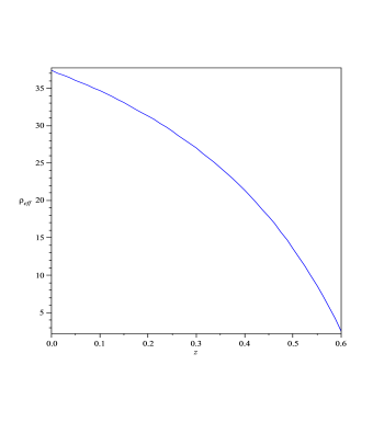
Figure 1: Variation of the effective energy density versus the redshift.

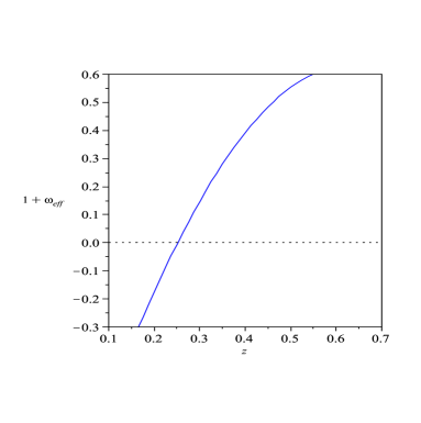
Figure 2: Variation of $1+\omega_{eff}$ versus the redshift.

Up to now we have shown that this modified GBIG scenario realizes the phantom-like behavior without introducing any phantom matter on the brane or in the bulk. This phantom-like behavior is a mimicry of $\Lambda$CDM scenario [6,7]. Now, the deceleration parameter defined as

$$q=-[\frac{\dot{H}}{H^{2}}+1]$$ (33)

takes the following form in our model

$$q=-\Big{[}1-\frac{r\dot{R}f^{\prime\prime}(R)-\frac{\kappa_{5}^{2}}{6H^{2}}(\dot{\rho}_{m}+\dot{\rho}_{curv})}{1+8\alpha H^{2}+2rHf^{\prime}(R)}\Big{]}\,.$$ (34)

Figure $3$ shows behavior of $q$ versus $z$. The universe has entered an accelerating phase in the past at $z\simeq 0.84$.

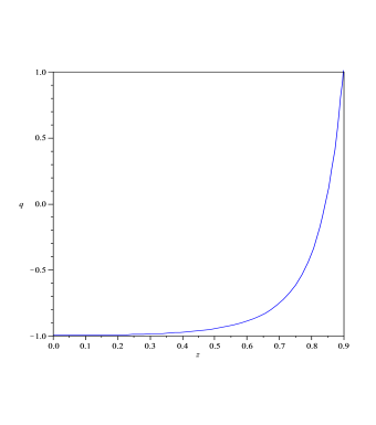
Figure 3: Variation of the deceleration parameter versus redshift.

The variation of $H$ with redshift gives another part of important information about the cosmology of this model. It is given by

$$\frac{\dot{H}}{H_{0}^{2}}=-\frac{1}{H_{0}^{2}}\frac{r\dot{R}H^{2}f^{\prime\prime}(R)-\frac{\kappa_{5}^{2}}{6}(\dot{\rho}_{m}+\dot{\rho}_{curv})}{1+8\alpha H^{2}+2rHf^{\prime}(R)}.$$ (35)

Figure $4$ shows the variation of $\frac{\dot{H}}{H_{0}^{2}}$ versus redshift. Since $\dot{H}<0$ always, the model universe described here will not acquire super-acceleration and big-rip singularity in the future.

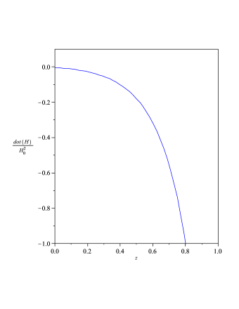
Figure 4: Variation of $\frac{\dot{H}}{H_{0}^{2}}$ versus the redshift.

Since we have not introduced any phantom field on the brane or in the bulk, we expect that the null energy condition to be respected at least in some subspaces of the model parameter space. Figure $5$ shows the status of the null energy condition in this setup. As this figure shows, phantom-like behavior occurs in this setup without violation of the null energy condition. We note that this model mimics a $\Lambda$CDM model in several respects and in this sense it is important to confront its parameter space with recent observation to see its viability.

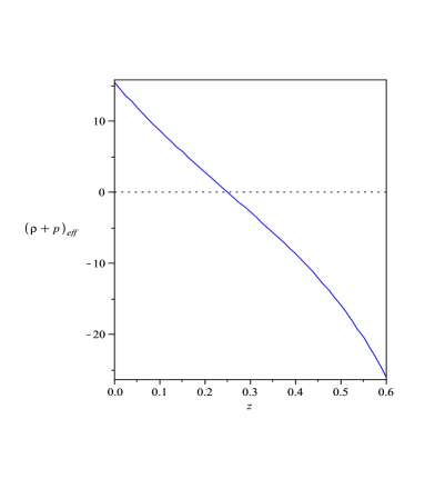
Figure 5: Variation of $\rho_{eff}+P_{eff}$ versus the redshift. Null energy condition is respected in the phantom phase of the model.

Finally we focus on the appropriate ranges of $n$ that crossing of the phantom divide line can be realized. Our analysis shows that $\omega_{curv}$ as defined by (19) crosses the phantom divide line smoothly if  $2.42\leq n\leq 4.68$. Also, $\omega_{total}$ crosses the phantom divide line if $2.44\leq n\leq 4.74$. And finally, $\omega$ as defined in equation (23), crosses the phantom line if $2.43\leq n\leq 5.15$. In our model, this crossing occurs at $z\simeq 0.27$ which lies well in the vicinity of the observationally supported value of $z\simeq 0.25$. Figure $6$ shows the behavior of these equation of state parameters versus $z$ for $n=4$. As this figure shows, crossing of the phantom divide evolves from quintessence to phantom phase in the same way as observations suggest.

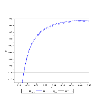
Figure 6: Smooth crossing of the phantom divide line.

3 Summary

In this paper we have constructed a modified GBIG scenario: it contains Gauss-Bonnet term as the UV sector of the theory and Induced Gravity effect as IR side of the model. The induced gravity on the brane is modified in the spirit of $f(R)$ gravity. The cosmological dynamics in this braneworld setup mimics a $\Lambda$CDM model in several respects: it realizes phantom-like behavior without introducing any phantom matter on the brane. The effective energy density increases with cosmic time and effective equation of state parameter crosses the phantom divide line smoothly in the same way as observations suggest. This crossing behavior occurs at $z\simeq 0.27$ which lies well in the vicinity of the observationally supported value of $z\simeq 0.25$. The phantom-like behavior realized in this model happens without violation of the null energy condition in the phantom phase. Finally, to have smooth crossing of the phantom divide line by $\omega_{eff}$, the value of parameter $n$ in the Hu-Sawicki model should lie in the range $2.42\leq n\leq 4.68$.

References

- [1] A. G. Riess et al, Astrophys. J. 607 (2004) 665; P. Astier et al, Astron. Astrophys. 447 (2006) 31; W. M. Wood-Vasey et al, Astrophys. J. 666 (2007) 694-715 [arXiv:astro-ph/0701041]; D. N. Spergel et al, Astrophys. J. Suppl 170 (2007) 377; G. Hinshaw et al, Astrophys. J. Suppl , 288 (2007)170; M. Colless et al, Mon. Not. R. Astron. Soc. 328 (2001) 1039; M. Tegmark et al, Phys. Rev. D 69 (2004) 103501; S. Cole et al., Mon. Not. R. Astron. Soc. 362 (2005) 505; V. Springel, C. S. Frenk, and S. M. D. White, Nature (London) 440 (2006) 1137; S. P. Boughn, and R. G. Crittenden, Nature 427 (2004) 24; S. P. Boughn, and R. G. Crittenden, Mon. Not. R. Astron. Soc. 360 (2005) 1013; P. Fosalba, E. Gaztanaga, and F.J. Castander, Astrophys. J. 597 (2003) L89; P. Fosalba, and E. Gaztanaga, Mon. Not. R. Astron. Soc. 350 (2004) L37; J. D. McEwen et al, Mon. Not. R. Astron. Soc. 376 (2007) 1211; M. R. Nolta, Astrophys. J., 608 (2004)10, P. Vielva et al, Mon. Not. R. Astron. Soc. 365 (2006) 891; C. R. Contaldi, H. Hoekstra, and A. Lewis, Phys. Rev. Lett. 90 (2003) 221303; E. Komatsu et al. [WMAP Collaboration], Astrophys. J. Suppl. 180 (2009) 330, [arXiv:0803.0547].
- [2] E. J. Copeland, M. Sami and S. Tsujikawa, Int. J. Mod. Phys. D 15 (2006) 1753, [ arXiv:hep-th/0603057]; S. Nojiri and S. D. Odintsov, Phys. Rev. D 70 (2004) 103522; R. R. Caldwell, Phys. Lett. B 545 (2002) 23-29; N. Arkani-Hamed, P. Creminelli, S. Mukohyama and M. Zaldarriaga, JCAP 0404 (2004) 001; F. Piazza and S. Tsujikawa, JCAP 0407 (2004) 004; H. Wei and R. G. Cai, Phys. Rev. D 73 (2006) 083002; A. Vikman, Phys. Rev. D 71 (2005) 023515, [arXiv:astro-ph/0407107]; A. Anisimov, E. Babichev and A. Vikman, JCAP 0506 (2005)006; B. Wang, Y.G. Gong and E. Abdalla, Phys. Lett. B 624 (2005) 141; S. Nojiri and S. D. Odintsov, [arXiv:hep-th/0506212]; S. Nojiri, S. D. Odintsov and S. Tsujikawa, [arXiv:hep-th/0501025]; E. Elizalde, S. Nojiri, S. D. Odintsov and P. Wang, Phys. Rev. D 71 (2005) 103504; W. Zhao and Y. Zhang, Phys. Rev.D 73 (2006)123509; P. S. Apostolopoulos and N. Tetradis, [arXiv:hep-th/0604014]; U. Alam , V. Sahni and A. A. Starobinsky, JCAP 06 (2004) 008; S. Nesseris and L. Perivolaropoulos, Phys. Rev. D 72 (2005) 123519; M. Libanov, E. Papantonopoulos, V. Rubakov, M. Sami and S. Tsujikawa, JCAP 0708 (2007) 010, M. R. Setare and E. N. Saridakis, [ arXiv:0810.0645]; R. J. Scherrer and A. A. Sen, Phys. Rev. D 78 (2008) 067303, [arXiv:0808.1880]; F. Briscese, E. Elizalde, S. Nojiri and S. D. Odintsov, Phys. Lett. B 646 (2007) 105-111; K. Nozari, M. R. Setare, T. Azizi and N. Behrouz, [arXiv:0810.1427]; M. Sami, [arXiv:0901.0756]; G. Caldera-Cabral, R. Maartens, L. A. Urena-Lopez, Phys. Rev. D 79 ( 2009) 063518, [ arXiv:0812.1827]; V. Sahni and A. Starobinsky, Int. J. Mod. Phys. D 15 (2006) 2105, [ arXiv:astro-ph/0610026]; V. Sahni, Lect. Notes Phys. 653 (2004) 141, [arXiv:astro-ph/0403324].
- [3] G. Dvali, G. Gabadadze and M. Porrati, Phys. Lett. B 485 (2000) 208, [hep-th/0005016]; G. Dvali and G. Gabadadze, Phys. Rev. D 63 (2001) 065007; G. Dvali, G. Gabadadze, M. Kolanovi and F. Nitti, Phys. Rev. D 65 (2002) 024031; C. Deffayet, Phys. Lett. B 502 (2001) 199; C. Deffayet, G. Dvali and G. Gabadadze, Phys. Rev. D 65 (2002) 044023; C. Deffayet, S. J. Landau, J. Raux, M. Zaldarriaga and P. Astier, Phys. Rev. D 66 (2002) 024019.
- [4] K. Koyama, Class. Quantum Grav. 24 (2007) R231, [arXiv:0709.2399]; C. de Rham and A. J. Tolley, JCAP 0607 (2006) 004, [arXiv:hep-th/0605122]
- [5] M. Sami, [arXiv:0904.3445]; M. Cadoni and P. Pani, [arXiv:0812.3010]; see also Y. Shtanov, V. Sahni, A. Shafieloo and A. Toporensky, JCAP 04 (2009) 023, [arXiv:0901.3074]
- [6] V. Sahni and Y. Shtanov, JCAP 0311 (2003) 014, [arXiv:astro-ph/0202346]; V. Sahni [arXiv:astro-ph/0502032]; A. Lue and G. D. Starkman, Phys. Rev. D 70 (2004) 101501, [arXiv:astro-ph/0408246]; L. P. Chimento, R. Lazkoz, R. Maartens and I. Quiros, JCAP 0609 (2006) 004, [arXiv:astro-ph/0605450]; R. Lazkoz, R. Maartens and E. Majerotto [arXiv:astro-ph/0605701]; R. Maartens and E. Majerotto [arXiv:astro-ph/0603353]; M. Bouhmadi-Lopez, Nucl. Phys. B 797 (2008) 78-92, [arXiv:astro-ph/0512124]; M. Bouhmadi-Lopez and A. Ferrera, JCAP 0810 (2008) 011, [arXiv:0807.4678].
- [7] M. Bouhamdi-Lopez, [arXiv:0905.1962][hep-th]. See also K. Nozari and F. Kiani, JCAP 07 (2009) 010, [ arXiv:0906.3806].
- [8] D. J. Gross and J. H. Sloan, Nucl. Phys. B 291 (1987) 41.
- [9] C. Charmousis and J. F. Dufaux, Class. Quant. Grav. 19 (2002) 4671, [arXiv:hep-th/0202107]; S. C. Davis, Phys. Rev. D 67 (2003) 024030, [arXiv:hep-th/0208205]; P. Binetruy, C. Charmousis, S. C. Davis and J. F. Dufaux, Phys. Lett. B 544 (2002) 183, [arXiv:hep-th/0206089].
- [10] K. Maeda and T. Torii, Phys. Rev. D 69 (2004) 024002, [arXiv:hep-th/0309152]; see also A. N. Aliev, H. Cebeci and T. Dereli, Class. Quant. Grav. 23 (2002) 591, [arXiv:hep-th/0507121]; A. N. Aliev, H. Cebeci and T. Dereli, Class. Quant. Grav. 24 (2007) 3425, [arXiv:gr-qc/0703011].
- [11] J. E. Lidsey and N. J. Nunes, Phys. Rev. D 67 (2003) 103510, [arXiv:astro-ph/0303168].
- [12] P. S. Apostolopoulos, N. Brouzakis, N. Tetradis and E. Tzavara, Phys. Rev. D 76 (2007) 084029, [arXiv:hep-th/0708.0469].
- [13] J. F. Dufaux, J. E. Lidsey, R. Maartens and M. Sami, Phys. Rev. D 70 (2004) 083525, [arXiv:hep-th/0404161].
- [14] S. Tsujikawa, M. Sami and R. Maartens, Phys. Rev. D 70 (2004) 063525, [arXiv:astro-ph/0406078].
- [15] S. Nojiri, S. D. Odintsov and S. Ogushi, Int. J. Mod. Phys. A 17 (2002) 4809, [arXiv:hep-th/0205187]; G. Kofinas, R. Maartens and E. Papantonopoulos, JHEP 0310 (2003) 066, [arXiv:hep-th/0307138]; R. G. Cai, H. S. Zhang and A. Wang, Commun. Theor. Phys. 44 (2005) 948, [arXiv:hep-th/0505186]; R. A. Brown, [arXiv:gr-qc/0602050]; M. Heydari-Fard and H. R. Sepangi, Phys. Rev. D 75 (2007) 064010, [arXiv:gr-qc/0702061]. See also: T. Koivisto and D. F. Mota, Phys. Lett. B 644 ( 2007) 104, [astro-ph/0606078]; T. Koivisto and D. F. Mota, Phys. Rev. D 75 (2007) 023518, [hep-th/0609155].
- [16] R. A. Brown, [arXiv:gr-qc/0701083]; R. A. Brown et al, JCAP 0511, 008 (2005), [arXiv:gr-qc/0508116]; K. Nozari and B. Fazlpour, JCAP 0806 (2008) 032, [ arXiv:0805.1537].
- [17] S. Alexander et al, Phy. Rev. D 62 (2000) 103509.
- [18] S. Nojiri and S. D. Odintsov, Int. J. Geom. Meth. Mod. Phys. 4 (2007) 115, [hep-th/0601213]; S. Nojiri and S. D. Odintsov, [arXiv:0807.0685]; T. P. Sotiriou and V. Faraoni, [arXiv:0805.1726]; S. Capozziello and M Francaviglia, Gen. Relativ. Gravit. 40 (2008) 357. See also R. Durrer and R. Maartens, [arXiv:0811.4132]; S. Nojiri and S. D. Odintsov, [arXiv:0807.0685]; K. Bamba, S. Nojiri and S. D. Odintsov, JCAP 0810 (2008) 045, [arXiv:0807.2575]; S. Jhingan, S. Nojiri, S. D. Odintsov, M. Sami, I. Thongkool and S. Zerbini, Phys. Lett.B 663 (2008)424, [ arXiv:0803.2613]; G. Cognola, E. Elizalde, S. Nojiri, S.D. Odintsov, L. Sebastiani, S. Zerbini, Phys. Rev. D 77 (2008) 046009, [ arXiv:0712.4017]; S. Nojiri and S. D. Odintsov, Phys. Lett. B 659 (2008) 821, [arXiv:0708.0924]; S. Nojiri and S. D. Odintsov, Phys. Rev. D 77 (2008) 026007, [arXiv:0710.1738]
- [19] S. M. Carroll, V. Duvvuri, M. Trodden and M. S. Turner, Phys. Rev. D70 (2004) 043528, [arXiv:astro-ph/0306438].
- [20] A. D. Dolgov and M. Kawasaki, Phys. Lett. B573 (2003) 1, [arXiv:astro-ph/0307285]. See also the issue of confrontation with solar system tests in: C.-G. Shao, R.-G. Cai, B. Wang and R.-K. Su, Phys. Lett. B633 (2006) 164, [arXiv:gr-qc/0511034]; A. L. Erickcek, T. L. Smith and M. Kamionkowski, Phys. Rev.D74 (2006) 121501, [arXiv:astro-ph/0610483].
- [21] V. Miranda, S. E. Jorás and I. Waga, [arXiv:0905.1941][astro-ph.CO]
- [22] P. S. Apostolopoulos, N. Brouzakis, N. Tetradis and E. Tzavara, Phys. Rev.D 76 (2007) 084029, [arXiv:0708.0469].
- [23] R. Dick, Class. Quant. Grav. 18 (2001) R1-R24, [arXiv:hep-th/0105320]; K. Nozari, JCAP 0709 (2007) 003, [arXiv:0708.1611]
- [24] S. Capozziello, V. F. Cardone and V. Salzano, Phys. Rev. D78 (2008) 063504, [arXiv:0802.1583]
- [25] L. Perivolaropoulos, JCAP 0510 (2005) 001; S. Nesseris, L. Perivolaropoulos, JCAP 0701 (2007) 018, [ arXiv:astro-ph/0610092]; M. Kunz and D. Sapone, Phys. Rev. D 74 (2006) 123503, [arXiv:astro-ph/0609040]; S. Das, S. Ghosh, J.-W. van Holten and S. Pal, [arXiv:0906.1044]; B. M. Leith and I. P. Neupane, JCAP 0705 (2007) 019, [arXiv:hep-th/0702002]; S. Nojiri and S. D. Odintsov, Gen. Rel. Grav. 38 (2006) 1285; H. Stefancic, Phys. Rev. D71 (2005) 124036; W. Fang, W. Hu and A. Lewis, Phys. Rev. D78 (2008) 087303, [arXiv:0808.3125]; M. R. Setare and E. N. Saridakis, Phys. Lett. B 670 (2008) 1, [ arXiv:0810.3296]; M. R. Setare and E. N. Saridakis, JCAP 0903 (2009) 002, [arXiv:0811.4253]; M. R. Setare and E. N. Saridakis, [arXiv:0810.0645]; M. R. Setare and A. Rozas-Fernndez, [arXiv:0906.1936]
- [26] S.D. Sadatian and K. Nozari, Europhys. Lett. 82 (2008) 49001, [arXiv:0803.2398]; K. Nozari and S. D. Sadatian, Eur. Phys. J. C58 (2008) 499, [ arXiv:0809.4744]; K. Nozari and S. D. Sadatian, JCAP 0901 (2009) 005, [arXiv:0810.0765].
- [27] See for instance: K. Nozari and M. Pourghasemi, JCAP 10 (2008) 044, [arXiv:0808.3701]; K. Bamba, C. Q. Geng, S. Nojiri and S. D. Odintsov, [arXiv:hep-th/0810.4296].
- [28] W. Hu and I. Sawicki, Phys. Rev. D 76 (2007) 064004, [arXiv:0705.1158 [astro-ph]].
- [29] A. A. Starobinsky, JETP Lett. 86 (2007) 157, [arXiv:0706.2041 [astro-ph]].
- [30] Y. S. Song, W. Hu and I. Sawicki, Phys. Rev. D 75 (2007) 044004, [arXiv:astro-ph/0610532].
- [31] L. Pogosian and A. Silvestri, Phys. Rev. D 77 (2008) 023503, [arXiv:0709.0296 [astro-ph]].
- [32] S. Capozziello, V. F. Cardone and A. Troisi, Phys. Rev. D 71 (2005) 043503, [arXiv:astro-ph/0501426].
- [33] Y. -F. Cai, T. Qiu, Y. -S. Piao, M. Li and X. Zhang, JHEP 0710 (2007) 071, [arXiv:0704.1090]. See also Y. -F. Cai, T. Qiu, R. Brandenberger, Y. -S. Piao and X. Zhang, JCAP 0803 (2008) 013, [arXiv:0711.2187].