Abstract

In this article, we use the light-cone QCD sum rules to relate the $\Lambda_{b}$ baryon light-cone distribution amplitudes to the Isgur-Wise function $\xi(\omega)$ of the $\Lambda_{b}\to\Lambda_{c}$ transition, and obtain a simple relation. The numerical value of the Isgur-Wise function $\xi(\omega)$ is consistent with the prediction of the QCD sum rules.

PACS numbers: 12.38.Lg; 14.20.Mr, 14.20.Lq

Key Words: $\Lambda_{Q}$ baryon, Isgur-Wise function, Light-cone QCD sum rules

1 Introduction

The semileptonic decay $b\to c$ is an important process in extracting the CKM matrix element $V_{cb}$ and serves as a laboratory for studying the nonperturbative QCD effects. In the baryon sector, the semileptonic decay $\Lambda_{b}\to\Lambda_{c}\ell\bar{\nu}_{\ell}$, which takes place through the process $b\to cW\to c\ell\bar{\nu}_{\ell}$ at the quark level, has attracted much attention. The charm and bottom baryons (e.g. $\Lambda_{c}$ and $\Lambda_{b}$) which contain a heavy quark and two light quarks are particularly interesting for studying dynamics of the light quarks in the presence of a heavy quark. They behave as the QCD analogue of the familiar hydrogen bounded by the electromagnetic interaction, and serve as an excellent ground for testing predictions of the constituent quark models and heavy quark symmetry [1, 2].

In the heavy quark limit, we can express the hadronic form-factor $\Lambda_{b}\to\Lambda_{c}$ in terms of the Isgur-Wise function $\xi(\omega)$ [2],

$$\langle\Lambda_{c}(v^{\prime})|\bar{c}_{v^{\prime}}(0)\Gamma b_{v}(0)|\Lambda_{b}(v)\rangle=\xi(\omega)\overline{U}_{\Lambda_{c}}(v^{\prime})\Gamma U_{\Lambda_{b}}(v)\,,$$ (1)

where the $v$ and $v^{\prime}$ are velocities of the heavy quarks $b$ and $c$ respectively, $\omega=v\cdot v^{\prime}$, and the $U(v)$ is the Dirac spinor. The Isgur-Wise function $\xi(\omega)$ is normalized to 1 at zero recoil $\omega=1$. In the weak decay $b\to cW$, the light degrees of freedom undergo a corresponding transition due to the gluon exchanges with the heavy quarks, and the Isgur-Wise function $\xi(\omega)$ has copious information about the dynamics of the light degrees of freedom. The physical region of the $\omega$ ($=\frac{M_{\Lambda_{b}}^{2}+M_{\Lambda_{c}}^{2}-q^{2}}{2M_{\Lambda_{b}}M_{\Lambda_{c}}}$) is rather small, about $1.0-1.43$. The existing theoretical estimations of the slope parameter $\rho^{2}$ vary from $0.5$ to $1.5$, one can consult Ref.[3] for more literatures. Using an exponential parametrization $\xi(\omega)=\exp\left[-\rho^{2}(\omega-1)\right]$, the DELPHI Collaboration obtain a value $\rho^{2}=1.59\pm 1.10$; after taking into account the observed event rates and adding the normalization condition $\xi(1)=1$, they reach the value $\rho^{2}=2.03\pm 0.46^{+0.72}_{-1.00}$ [4], the uncertainty is very large.

In Refs.[6, 7], Khodjamirian et al derive new sum rules for the $B\to\pi,K,\rho,K^{*}$ form-factors from the correlation functions expanded near the light-cone in terms of the $B$-meson distribution amplitudes, and suggest QCD sum rules motivated models for the three-particle $B$-meson light-cone distribution amplitudes, which satisfy the exact relations between the two-particle and three-particle $B$-meson light-cone distribution amplitudes [8]. The $B$-meson light-cone QCD sum rules have been applied to the form-factors $B\to a_{1}(1260)$ [9] and $B\to D,D^{*}$ [10]. In Ref.[11], De Fazio et al study the sum rules for the heavy-to-light transition form-factors at large recoil derived from the correlation functions with interpolating currents for the light pseudoscalar (or vector) fields in soft-collinear effective theory and the $B$-meson light-cone distribution amplitudes.

In Ref.[5], Ball et al perform a complete classification of the three-quark distribution amplitudes of the $\Lambda_{b}$ baryon in QCD in the heavy quark limit and discuss the relevant features, and derive a renormalization-group equation which governs the scale-dependence of the leading-twist light-cone distribution amplitudes. Furthermore, they suggest simple models of the light-cone distribution amplitudes and estimate the relevant parameters based on the first few moments using the QCD sum rules.

In this article, we study the Isgur-Wise function $\xi(\omega)$ of the transition $\Lambda_{b}\to\Lambda_{c}$ with the $\Lambda_{b}$-baryon light-cone QCD sum rules, i.e. we use the light-cone sum rules to relate the $\Lambda_{b}$-baryon light-cone distribution amplitudes to the Isgur-Wise function $\xi(\omega)$.

The article is arranged as: in Section 2, we derive the Isgur-Wise function $\xi(\omega)$ with the light-cone QCD sum rules; in Section 3, the numerical result and discussion; and in Section 4 is reserved for conclusion.

2 Isgur-Wise function $\xi(\omega)$ with light-cone QCD sum rules

We study the Isgur-Wise function $\xi(\omega)$ with the two-point correlation functions $\Pi^{i}_{\mu}(p,q)$,

$$\Pi^{i}_{\mu}(p,q) = i\int d^{4}x\,e^{ip\cdot x}\langle 0|T\left\{\eta_{i}(x)J_{\mu}(0)\right\}|\Lambda_{b}(v)\rangle\,,$$ (2)

where

$$\eta_{1}(x) = \epsilon_{ijk}u^{i}(x)C\gamma_{5}\not\!nd^{j}(x)c^{k}_{v}(x)\,,$$

$$\eta_{2}(x) = \epsilon_{ijk}u^{i}(x)C\gamma_{5}d^{j}(x)c^{k}_{v}(x)\,,$$

$$\eta_{3}(x) = \epsilon_{ijk}u^{i}(x)C\gamma_{5}i\sigma_{\bar{n}n}d^{j}(x)c^{k}_{v}(x)\,,$$

$$J_{\mu}(x) = \bar{c}_{v^{\prime}}(x)\gamma_{\mu}(1-\gamma_{5})b_{v}(x)\,,$$ (3)

the quark currents $\eta_{i}(x)$ ($i=1,2,3$) interpolate the heavy baryon $\Lambda_{c}$, $\sigma_{\bar{n}n}=\sigma_{\mu\nu}\bar{n}^{\mu}n^{\nu}$, the $n_{\mu}$ and $\bar{n}_{\mu}$ are light-like vectors and the $C$ is the charge conjugation matrix.

Based on the assumption of the quark-hadron duality [12, 13], we insert a complete set of intermediate states with the same quantum numbers as the current operators $\eta_{i}(x)$ into the correlation functions $\Pi^{i}_{\mu}(p,q)$ to obtain the hadronic representation. After isolating the ground state contribution from the pole term of the $\Lambda_{c}$ baryon, the correlation functions $\Pi^{i}_{\mu}(p,q)$ can be expressed in the following form,

$$\Pi^{i}_{\mu}(p,q) = \frac{f^{i}_{\Lambda}}{\bar{\Lambda}-p\cdot v^{\prime}}\frac{1+\not\!v^{\prime}}{2}\gamma_{\mu}\xi(\omega)U(v)+\cdots\,,$$ (4)

where the $\bar{\Lambda}$ is the bound energy in the heavy quark limit, $\bar{\Lambda}=M_{\Lambda_{b}}-m_{b}=M_{\Lambda_{c}}-m_{c}$. We have used the standard definition for the pole residues (or the coupling constants) $f^{i}_{\Lambda}$,

$$\epsilon_{ijk}\langle 0|\left[u^{i}(0)C\gamma_{5}\not\!nd^{j}(0)\right]h^{k}_{v}(0)|\Lambda(v)\rangle = f^{2}_{\Lambda}U(v)\,,$$

$$\epsilon_{ijk}\langle 0|\left[u^{i}(0)C\gamma_{5}d^{j}(0)\right]h^{k}_{v}(0)|\Lambda(v)\rangle = f^{1}_{\Lambda}U(v)\,,$$

$$\epsilon_{ijk}\langle 0|\left[u^{i}(0)C\gamma_{5}i\sigma_{\bar{n}n}d^{j}(0)\right]h^{k}_{v}(0)|\Lambda(v)\rangle = f^{3}_{\Lambda}U(v)\,,$$ (5)

and $f^{3}_{\Lambda}=2f^{1}_{\Lambda}$.

In the following, we briefly outline the operator product expansion for the correlation functions $\Pi^{i}_{\mu}(p,q)$ in perturbative QCD. The calculations are performed at the large space-like momentum region $|p^{2}|\gg\Lambda_{QCD}$ and $q^{2}\gg\Lambda_{QCD}$. We write down the propagator of the $c$ quark and the light-cone distribution amplitudes of the $\Lambda_{b}$ baryon in the heavy quark limit,

$$\langle 0|T\{h_{v}(x)\,\bar{h}_{v}(0)\}|0\rangle = \frac{1+\not\!v}{2}\int_{0}^{\infty}d\lambda\delta^{4}(x-v\lambda)\,,$$ (6)

$$\epsilon_{ijk}\langle 0|\left[u^{i}(t_{1}n)C\gamma_{5}\not\!nd^{j}(t_{2}n)\right]h^{k}_{v}(0)|\Lambda_{b}(v)\rangle = f^{2}_{\Lambda}\Psi_{2}(t_{1},t_{2})U(v)\,,$$

$$\epsilon_{ijk}\langle 0|\left[u^{i}(t_{1}n)C\gamma_{5}d^{j}(t_{2}n)\right]h^{k}_{v}(0)|\Lambda_{b}(v)\rangle = f^{1}_{\Lambda}\Psi_{3}^{s}(t_{1},t_{2})U(v)\,,$$

$$\epsilon_{ijk}\langle 0|\left[u^{i}(t_{1}n)C\gamma_{5}i\sigma_{\bar{n}n}d^{j}(t_{2}n)\right]h^{k}_{v}(0)|\Lambda_{b}(v)\rangle = f^{3}_{\Lambda}\Psi_{3}^{\sigma}(t_{1},t_{2})U(v)\,,$$ (7)

where

$$\Psi(t_{1},t_{2}) = \int_{0}^{\infty}\!\!d\omega_{1}\int_{0}^{\infty}\!\!d\omega_{2}\,e^{-it_{1}\omega_{1}-it_{2}\omega_{2}}\psi(\omega_{1},\omega_{2})$$ (8)

$$= \int_{0}^{\infty}\!\!\omega\,d\omega\int_{0}^{1}du\,e^{-i\omega(t_{1}u+it_{2}\bar{u})}\widetilde{\psi}(\omega,u)\,,$$

$$\widetilde{\psi}_{2}(\omega,u) = \omega^{2}u(1-u)\left[\frac{1}{\varepsilon_{0}^{4}}e^{-\omega/\varepsilon_{0}}+a_{2}C_{2}^{3/2}(2u-1)\frac{1}{\varepsilon_{1}^{4}}e^{-\omega/\varepsilon_{1}}\right]\,,$$

$$\widetilde{\psi}^{s}_{3}(\omega,u) = \displaystyle{\frac{\omega}{2\varepsilon_{3}^{3}}}\,e^{-\omega/\varepsilon_{3}}\,,$$

$$\qquad\widetilde{\psi}^{\sigma}_{3}(\omega,u) = \frac{\omega}{2\varepsilon_{3}^{3}}(2u-1)\,e^{-\omega/\varepsilon_{3}}\,,$$ (9)

$v_{\mu}=(n_{\mu}+\bar{n}_{\mu})/2$, $v\cdot n=1$, $n\cdot\bar{n}=2$, $\widetilde{\psi}(\omega,u)=\psi(u\omega,\bar{u}\omega)$, and $\bar{u}=1-u$. The $\widetilde{\psi}$ denotes the light-cone distribution amplitudes $\widetilde{\psi}_{2}$, $\widetilde{\psi}_{3}^{s}$ and $\widetilde{\psi}_{3}^{\sigma}$. The $\omega_{1}$ and $\omega_{2}$ are the energies of the $u$ and $d$ quarks respectively, and $\omega=\omega_{1}+\omega_{2}$, $\omega_{1}=u\omega$ and $\omega_{2}=\bar{u}\omega$. The $\varepsilon_{0}$, $\varepsilon_{1}$, $a_{2}$ and $\varepsilon_{3}$ are nonperturbative parameters.

Substituting the above $c$ quark propagator and the corresponding $\Lambda_{b}$ baryon light-cone distribution amplitudes into the correlation functions $\Pi^{i}_{\mu}(p,q)$, and completing the integrals over the variables $x$ and $\lambda$, finally we obtain the representation at the level of quark-gluon degrees of freedom,

$$\Pi^{i}_{\mu}(p,q) = f_{\Lambda}^{i}\frac{1+\not\!v^{\prime}}{2}\gamma_{\mu}U(v)\int_{0}^{\infty}\omega^{\prime}d\omega^{\prime}\int_{0}^{1}du\frac{1}{\omega\omega^{\prime}-p\cdot v^{\prime}}\widetilde{\psi}(\omega^{\prime},u)+\cdots\,,$$ (10)

After matching with the hadronic representation below the continuum threshold $s_{0}$, we obtain three sum rules for the Isgur-Wise function $\xi(\omega)$,

$$\xi(\omega)\exp\left[-\frac{\bar{\Lambda}}{T}\right] = \int_{0}^{s_{0}}ds\int_{0}^{1}du\frac{s}{\omega^{2}}\widetilde{\psi}\left(\frac{s}{\omega},u\right)\exp\left[-\frac{s}{T}\right]\,,$$ (11)

where the $T$ is the Borel parameter, the $\widetilde{\psi}$ denotes the $\widetilde{\psi}_{2}$, $\widetilde{\psi}_{3}^{s}$ and $\widetilde{\psi}_{3}^{\sigma}$, thereafter we will denote the corresponding sum rule as SRI, SRII, and SRIII respectively. The present sum rules do not suffer from uncertainties which originate from the hadronic parameters $f_{\Lambda}^{i}$ as they cancel out between the left side and the right side. In the light-cone QCD sum rules, the hadronic parameters always make large contributions to the uncertainties. The four-particle light-cone distribution amplitudes of the $\Lambda_{b}$ baryon are unknown, we only take into account the contributions from the three-quark light-cone distribution amplitudes. In case of the nucleon, the contributions proportional to the gluon $G_{\mu\nu}$ can give rise to four-particle (and five-particle) nucleon distribution amplitudes with a gluon (or quark-antiquark pair) in addition to the three valence quarks, their corrections are usually not expected to play any significant roles [14].

3 Numerical result and discussion

The input parameters are taken as $\bar{\Lambda}=0.8\,\rm{GeV}$, $s_{0}=1.2\,\rm{GeV}$, $T=(0.4-0.8)\,\rm{GeV}$, $\varepsilon_{0}=200^{+130}_{-60}$ MeV, $\varepsilon_{1}=650^{+650}_{-300}$ MeV, $a_{2}=0.333^{+0.250}_{-0.333}$, and $\varepsilon_{3}=230$ MeV at the energy scale $\mu=1\,\rm{GeV}$ [5].

The nonperturbatuive parameters $\varepsilon_{0}$, $\varepsilon_{1}$, $\varepsilon_{3}$, $a_{2}$ in the light-cone distribution amplitudes are estimated by calculating the first few moments with the two-point QCD sum rules, the uncertainties are very large. In numerical calculation, we observe that the uncertainties originate from the nonperturbatuive parameters ($\varepsilon_{0}$, $\varepsilon_{1}$, $\varepsilon_{3}$) are out of control. In this article, we take the central values and make a crude estimation.

The values of the threshold parameter and Borel parameter $s_{0}=1.2\,\rm{GeV}$ and $T=(0.4-0.8)\,\rm{GeV}$ are determined by the two-point QCD sum rules. The physical region of the Isgur-Wise function $\xi(\omega)$ lies in the range $\omega=1-1.43$. In Fig.1, we plot the Isgur-Wise function $\xi(\omega)$ from the SRI and SRII, respectively. From the figure, we can see that the Isgur-Wise function $\xi(\omega)$ from the SRI is more stable with variation of the Borel parameter $T$. At the interval $T=(0.6-0.8)\,\rm{GeV}$, the curves of the $\xi(\omega)$ are more flat than that of the $T=(0.4-0.6)\,\rm{GeV}$ and the predictions are more robust, we can take the value $T=(0.6-0.8)\,\rm{GeV}$. Finally we obtain the values,

$$\xi(1) = 1.09\pm 0.05\,,$$

$$\xi(1) = 1.30\pm 0.08\,,$$ (12)

for the SRI and SRII, respectively. Here only the uncertainties originate from the Borel parameter $T$ are taken into account. Although the $\xi(1)$ deviates from the normalization condition $\xi(1)=1$, the central value $\xi(1)=1.09$ is rather good. From Eq.(9), we can see that the model light-cone distribution amplitudes are simple, more complicated distribution amplitudes maybe improve the predictions. Furthermore, we have neglected the contributions from the four-particle light-cone distribution amplitudes, their contributions maybe large enough to smear the discrepancy. As the four-particle light-cone distribution amplitudes of the $\Lambda_{b}$ baryon are unknown, we can not take into account their contributions.

Taking the exponential parametrization $\xi(\omega)=\exp\left[-\rho^{2}(\omega-1)\right]$ and the normalization condition $\xi(1)=1$, we obtain the values of the slope parameter $\rho^{2}=1.10$ and $\rho^{2}=0.85$ for the SRI and SRII respectively, which are consistent with the estimation $\rho^{2}=1.35\pm 0.12$ by the QCD sum rules [3], the QCD sum rules also support much smaller value $\rho^{2}=0.55\pm 0.15$ [15]; the present prediction is rather good with the simple model.

The SRIII involves the distribution amplitude $\widetilde{\psi}_{3}^{\sigma}$, the integral $\int_{0}^{1}du\widetilde{\psi}_{3}^{\sigma}(\omega^{\prime},u)=0$, so that $\xi(\omega)=0$, the prediction is very poor.

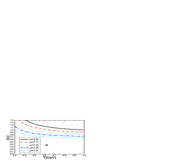
Figure 1: The Isgur-Wise function $\xi(\omega)$ with variation of the Borel parameter $T$. The $A$ and $B$ denote the values from the SRI and SRII, respectively.

In Ref.[5], Ball et al observe that the evolution effects drive the light-cone distribution amplitudes to generate a radiative tail that falls off as $\ln(\omega_{1}/\mu)/\omega_{1}$ or $\ln(\omega_{2}/\mu)/\omega_{2}$ at large energies, which is analogous to the evolution behavior of the $B$-meson light-cone distribution amplitude [16]. In this article, we obtain the sum rules without the radiative $\mathcal{O}(\alpha_{s})$ corrections, the ultraviolet behavior of the $\widetilde{\psi}$ plays no role at the leading order. Furthermore, the duality thresholds in the sum rules are well below the region where the effect of the tail becomes noticeable.

4 Conclusion

In this article, we use the light-cone QCD sum rules to relate the $\Lambda_{b}$ baryon light-cone distribution amplitudes to the Isgur-Wise function $\xi(\omega)$ of the $\Lambda_{b}\to\Lambda_{c}$ transition, and obtain a simple relation. The numerical value of the Isgur-Wise function $\xi(\omega)$ is consistent with the prediction of the QCD sum rules. If the four-particle light-cone distribution amplitudes are taken into account and the three-quark light-cone distribution amplitudes are improved, the prediction maybe better.

References

• [1] J. G. Koerner, D. Pirjol and M. Kraemer, Prog. Part. Nucl. Phys. 33 (1994) 787.
• [2] A. V. Manohar and M. B. Wise, Camb. Monogr. Part. Phys. Nucl. Phys. Cosmol. 10 (2000) 1.
• [3] M. Q. Huang, H. Y. Jin, J. G. Korner and C. Liu, Phys. Lett. B629 (2005) 27.
• [4] J. Abdallah et al, Phys. Lett. B585 (2004) 63.
• [5] P. Ball, V. M. Braun and E. Gardi, Phys. Lett. B665 (2008) 197.
• [6] A. Khodjamirian, T. Mannel and N. Offen, Phys. Lett. B620 (2005) 52.
• [7] A. Khodjamirian, T. Mannel and N. Offen, Phys. Rev. D75 (2007) 054013.
• [8] H. Kawamura, J. Kodaira, C. F. Qiao and K. Tanaka, Phys. Lett. B523 (2001) 111.
• [9] Z. G. Wang, Phys. Lett. B666 (2008) 477.
• [10] S. Faller, A. Khodjamirian, C. Klein and T. Mannel, Eur. Phys. J. C60 (2009) 603.
• [11] F. De Fazio, T. Feldmann and T. Hurth, JHEP 0802 (2008) 031.
• [12] M. A. Shifman, A. I. Vainshtein and V. I. Zakharov, Nucl. Phys. B147 (1979) 385,448.
• [13] L. J. Reinders, H. Rubinstein and S. Yazaki, Phys. Rept. 127 (1985) 1.
• [14] M. Diehl, T. Feldmann, R. Jakob and P. Kroll, Eur. Phys. J. C8 (1999) 409.
• [15] Y. B. Dai, C. S. Huang, M. Q. Huang and C. Liu, Phys. Lett. B387 (1996) 379.
• [16] B. O. Lange and M. Neubert, Phys. Rev. Lett. 91 (2003) 102001.