Reflection of neutrons from fan-like magnetic systems

Abstract

An analytical solution is found for neutron reflection coefficients from magnetic mirrors with fan-like magnetization. The main feature of the reflection curves related to this type of magnetization is pointed out. The results of calculations for some parameters of the system are presented. Time parity and detailed balance violation in the model are discussed.

I Introduction

Investigation of neutron reflection from multilayers belongs to the field of nanostructure research. Magnetic multilayered systems with magnetization vector varying in space can be grown artificially by consecutive evaporation or sputtering techniques of magnetic layers with different coercivity, or they can appear naturally under the action of anisotropic exchange forces kort ; buz ; lei ; calv . A representative example is a soft-magnetic layer (SL) which is magnetically coupled to a hard-magnetic layer (HL) goto ; dono ; kuncser ; hellwig , when the last one is magnetized non parallel with respect to the external field orientation. As a result, the SL becomes virtually separated into magnetic layers with different orientations of the magnetization vector, which turns from a direction almost parallel to the external field to a direction defined by the HL magnetization vector. This turn can go along a spiral, giving rise to a helicoidal structure, often referred to as spring magnet, or this turn can be confined in the plane perpendicular to the sample interface. In the last case, the magnetization in the SL is fan-like, and is referred to as perpendicular exchange-spring multilayer perp1 ; perp2 . Neutron scattering on helicoidal structures was investigated in Ref. aks . Here we consider the neutron scattering on a fan-like system. Such a magnetic state in fact consists of a large number of magnetic layers with magnetization slightly turned with respect to each other, and the neutron scattering on them can be calculated numerically by making use of generalized matrix methods rad ; polar ; ruhm ; deak . However it is possible to model the fan-like system by a magnet with continuous rotation of the magnetization vector, and to calculate neutron scattering on it analytically. We show here that neutron scattering on fan-like and helicoidal magnets are very similar. For instance, reflection curves for both configurations exhibit a resonance in some range of values of the normal wave vector component of the incident neutrons.

In the next section we find an analytical solution of the Schrödinger equation in a homogeneous medium with fan-like magnetization. In section III we calculate analytically the polarized neutron reflectivities from a semi-infinite magnetic media with fan-like magnetization in the absence of an external field. In this case, the quantization axis for the neutron spin $s$ is chosen along the axis $q$ of the magnetization rotation, and the neutron scattering becomes dependent on correlation $s$$q$, which violates time parity conservation and detailed balance theorem.

In section IV we find analytical expressions for reflectivity from a magnetic slab of finite thickness, also in the absence of an external field. The results are further used in section V to calculate the neutron reflection from a magnetic film with fan-like magnetic state and nonzero external field. In section VI we consider a SL/HL magnetic heterostructure and calculate the neutron reflectivity curves from the front side and from the back side of the sample, respectively like in the dono experiment. Finally, the results are summarized in section VII.

II Neutron propagation in a homogeneous medium with fan-like magnetization

Let’s consider a semi-infinite (z$>$0) mirror and an arbitrary external field. Magnetic induction in the medium consists of two parts: one part is constant, $\mbox{${\rm\bf B}$}=B(1,0,0)$ and directed along an $x$-axis. The other one, $\mbox{${\rm\bf b}$}(z)=b(0,\cos(2qz),\sin(2qz)$, rotates around $x$-axis (the factor 2 is selected for convenience). Our task is to find the neutron reflection from such a system. Therefore, we need to find the neutron wave function inside the mirror, i.e. to find a solution of the Schrödinger equation, which we shall represent in the form:

$$\bigg{(}\frac{d^{2}}{dz^{2}}-u_{0}-2b[\sigma_{y}\cos(2qz+2\varphi)+\sigma_{z}\sin(2qz+2\varphi)]-2B\sigma_{x}+k^{2}\bigg{)}|\psi(z)\rangle=0,$$ (1)

where $\sigma_{x}$,$\sigma_{y}$,$\sigma_{z}$ are the Pauli matrices, $u_{0}$ is the medium optical potential multiplied by the factor $2m/\hbar^{2}$ ($m$ is the neutron mass), and magnetic fields include the factor $|\mu|m/\hbar^{2}$ ($\mu$ is the neutron magnetic moment).

In the argument of the rotating field we included a mismatch phase $2\varphi$, which characterizes the angle between the external and the internal magnetic fields at the interface of the medium. In the real class of perpendicular exchange-spring magnetic multilayers perp1 ; perp2 the magnetization changes stepwise via magnetic domains with slightly turned magnetization, but for analytical calculations we can approximate such a change by a model of a continuous rotation of this magnetization.

For solution of (1) we use the well known relation:

$$\sigma_{y}\cos(2qz+2\varphi)+\sigma_{z}\sin(2qz+2\varphi)=\exp(-i\sigma_{x}(qz+\varphi))\sigma_{y}\exp(i\sigma_{x}(qz+\varphi)),$$ (2)

and represent the wave function $|\psi(z)\rangle$ in the form:

$$|\psi(z)\rangle=\exp(-i\sigma_{x}(qz+\varphi))|\phi(z)\rangle,$$ (3)

where

$$|\phi(0)\rangle=\exp(i\sigma_{x}\varphi)|\psi(0)\rangle$$ (4)

and $|\psi(0)\rangle$ corresponds to an arbitrary spin state.

Substitution of (2) and (3) into Eq. (1) gives:

$$\bigg{(}\frac{d^{2}}{dz^{2}}-2iq\sigma_{x}\frac{d}{dz}-u_{0}-2b\sigma_{y}-2B\sigma_{x}+k^{2}-q^{2}\bigg{)}|\phi(z)\rangle=0.$$ (5)

II.1 A solution by Calvo calv

Such a type of equation was solved in calv by substitution

$$|\phi(z)\rangle=\exp(ipz)|\xi\rangle$$ (6)

with constant parameter $p$ and some constant spinor state $|\xi\rangle$. After substitution we reduce (5) to

$$\bigg{(}-p^{2}+2q\sigma_{x}p-u_{0}-2b\sigma_{y}-2B\sigma_{x}+k^{2}-q^{2}\bigg{)}|\xi\rangle=0,$$ (7)

which is of the type

$$\mbox{\boldmath$\hat{M}$}|\xi\rangle=0$$ (8)

with constant matrix $\hat{M}$. This equation for nonzero $|\xi\rangle$ can be satisfied only if det$(\mbox{\boldmath$\hat{M}$})=0$. The last condition gives an equation for $p$, and for every its root $p_{i}$ there is the spinor state $|\xi_{i}\rangle$. Two positive roots give two spinor eigenstates going along $z$-axis, and two negative roots give the eigen states doing in opposite directions. It can be elucidated by analogy with the neutron propagation in a homogeneous magnetic field ${\rm\bf B}$ directed, say, along $x$-axis. The Schrödinger equation equation looks: $(d^{2}/dz^{2}-u_{0}-2B\sigma_{x}+k^{2})|\phi(z)\rangle=0$. Substitution of (6) reduces it to $(-p^{2}-u_{0}-2B\sigma_{x}+k^{2})|\xi\rangle=0$, which of the form (8), and the condition det$(\mbox{\boldmath$\hat{M}$})=0$ gives the equation $(p^{2}-k^{2}+u_{0})^{2}-4B^{2}=0$, from which we get 4 roots $p_{i}=\pm\sqrt{k^{2}-u_{0}\pm 2B}$ for 2 eigenstates $|\xi_{\pm x}\rangle$ polarized along and opposite $x$-axis.

It is well for description of the neutron propagation in a homogeneous space. The difficulties start, when we have to calculate neutron reflection from a magnetic mirror. In that case, even at a single interface matching of the wave function and its derivative gives in general 4 linear equations with 4 unknowns, and if we have two interfaces the number of equations doubles. Below we show how to avoid this huge number of equations and find an analytical solution for a general problem of the neutron reflection and transmission at a magnetic mirror of a finite thickness.

II.2 Our solution

Our solution will proceed along the lines of the work aks . We will substitute in Eq. (5) a solution for a wave, going to the right, in the form

$$|\phi(z)\rangle=\exp(i[a+\overrightarrow{\mbox{\boldmath$p$}}\mbox{\boldmath$\sigma$}]z)|\chi\rangle,$$ (9)

where $|\chi\rangle$ is an arbitrary spin state. This equation has four unknown parameters $a$ and $\overrightarrow{\mbox{\boldmath$p$}}$. A solution for a wave going to the left can be written as:

$$|\phi(z)\rangle=\exp(-i[a+\overleftarrow{\mbox{\boldmath$p$}}\mbox{\boldmath$\sigma$}]z)|\chi\rangle$$ (10)

containing again four unknown parameters $a$ and $\overleftarrow{\mbox{\boldmath$p$}}$. Here, $\mbox{\boldmath$\sigma$}=(\sigma_{x},\sigma_{y},\sigma_{z})$ is a vector of the Pauli matrices.

Substitution of (9) into (5) gives:

$$[-a^{2}-\overrightarrow{\mbox{\boldmath$p$}}^{2}-2a\overrightarrow{\mbox{\boldmath$p$}}\mbox{\boldmath$\sigma$}+2q\sigma_{x}(a+\overrightarrow{\mbox{\boldmath$p$}}\mbox{\boldmath$\sigma$})-u_{0}-2b\sigma_{y}-2B\sigma_{x}+k^{2}-q^{2}]|\phi(z)\rangle=0.$$ (11)

The new equation is of the type (8)

$$\mbox{\boldmath$\hat{M}$}|\phi(z)\rangle=0.$$ (12)

It contains a constant matrix $\hat{M}$, but instead of a constant spinor $|\xi\rangle$ it contains $|\phi(z)\rangle$, which according to (10) depends on $z$, contains an arbitrary spinor $|\chi\rangle$, and therefore is itself an arbitrary spinor. In such a case Eq. (12) can be satisfied only if $\mbox{\boldmath$\hat{M}$}=0$. This condition is equivalent to the following four equations:

$$-a^{2}-\overrightarrow{\mbox{\boldmath$p$}}^{2}+2q\overrightarrow{p}_{x}-u_{0}+k^{2}-q^{2}=0,$$ (13)

$$-2a\overrightarrow{p}_{x}+2qa-2B=0,\quad-2a\overrightarrow{p}_{y}-2iq\overrightarrow{p}_{z}-2b=0,\\ \quad-2a\overrightarrow{p}_{z}+2iq\overrightarrow{p}_{y}=0.$$ (14)

It follows from the last three equations that:

$$\overrightarrow{p}_{x}=q-\displaystyle\frac{B}{a},\quad\overrightarrow{p}_{y}=\frac{ab}{q^{2}-a^{2}},\quad\overrightarrow{p}_{z}=i\frac{qb}{q^{2}-a^{2}},\\ \quad\overrightarrow{\mbox{\boldmath$p$}}^{2}=\left(q-\displaystyle\frac{B}{a}\right)^{2}+\frac{b^{2}}{a^{2}-q^{2}}.$$ (15)

Substitution of (15) into (13) leads to:

$$-a^{2}+q^{2}-\displaystyle\frac{B^{2}}{a^{2}}-\frac{b^{2}}{a^{2}-q^{2}}-u_{0}+k^{2}-q^{2}=0,$$ (16)

which is the cubic equation for $a^{2}$.

Solution of the cubic equation

Denoting $x=a^{2}-q^{2}$ and $K^{2}=k^{2}-u_{0}-q^{2}$, we reduce (16) to

$$x^{3}-x^{2}(K^{2}-q^{2})+x(B^{2}+b^{2}-K^{2}q^{2})+b^{2}q^{2}=0.$$ (17)

A further change of variables $x=y+(K^{2}-q^{2})/3$ transforms it to:

$$y^{3}-\alpha y-\beta=0,$$ (18)

where

$$\alpha=\displaystyle\frac{(K^{2}-q^{2})^{2}}{3}-B^{2}-b^{2}+K^{2}q^{2},\qquad\beta=\displaystyle\frac{K^{2}-q^{2}}{3}\left(\alpha-\displaystyle\frac{(K^{2}-q^{2})^{2}}{9}\right)+b^{2}q^{2}.$$ (19)

Substituting $y=z+\alpha/3z$, reduces the Eq. (18) to $z^{3}+\alpha^{3}/27z^{3}-\beta=0$, and solution of it can be written as:

$$z_{n}=e^{2\pi in/3}\sqrt{\displaystyle\frac{\beta\pm\sqrt{\beta^{2}-4\alpha^{3}/27}}{2}},$$ (20)

where $n=0,1,2$. Therefore, the function $a(k)$ can be represented as:

$$a=\sqrt{q^{2}+\displaystyle\frac{K^{2}-q^{2}}{3}+z_{n}+\displaystyle\frac{\alpha}{3z_{n}}},$$ (21)

and the challenge is how to choose a single correct and physical root. We can look for the correct one between the roots of the form:

$$a=\sqrt{q^{2}+\displaystyle\frac{K^{2}-q^{2}}{3}+e^{2\pi in/3}\sqrt[3]{\displaystyle\frac{\beta-\sqrt{\beta^{2}-4\alpha^{3}/27}}{2}}+e^{-2\pi in/3}\displaystyle\frac{\alpha}{3}\sqrt[3]{\displaystyle\frac{2}{\beta-\sqrt{\beta^{2}-4\alpha^{3}/27}}}},$$ (22)

or equivalent ones:

$$a=\sqrt{q^{2}+\displaystyle\frac{K^{2}-q^{2}}{3}+e^{2\pi in/3}\sqrt[3]{\displaystyle\frac{\beta-\sqrt{\beta^{2}-4\alpha^{3}/27}}{2}}+e^{-2\pi in/3}\sqrt[3]{\displaystyle\frac{\beta+\sqrt{\beta^{2}-4\alpha^{3}/27}}{2}}}.$$ (23)

It is interesting, however, that at some energy interval these two expressions are not equivalent and (23) gives erroneous result, which will be discussed later.

The choice of roots

We need to choose such a solution which for small $b$, $B$ and $q$ is reduced to $a=\sqrt{k^{2}-u_{0}}$. To make a correct choice, we set $B=0$ and simplify Eq. (16) to the quadratic one:

$$-a_{s}^{2}+q^{2}-\frac{b^{2}}{a_{s}^{2}-q^{2}}-K^{2}=0,$$ (24)

where $a_{s}$ denotes $a(B=0)$. The solutions of (24) satisfying the above requirement reads:

$$a_{s}=\sqrt{q^{2}+\frac{1}{4}\bigg{(}\sqrt{K^{2}-2b}+\sqrt{K^{2}+2b}\bigg{)}^{2}}.$$ (25)

Now, with the help of computer we choose the integer $n$ in the phase $2\pi n/3$ of (22), or (23), which for $B=0$ gives $a(B=0)$ identical to (25). By trial and error method, we found that in the interval $0<k<k_{1}$, where $k_{1}$ has a value defined by Eq. $Re(\beta^{2}-4\alpha^{3}/27)=0$, the integer $n$ is 2 and both forms (22), (23) for the function $a(k)$ are equivalent; in the interval $k_{1}<k<k_{2}$, where $k_{2}=\sqrt{u_{0}+q^{2}+b}$, $n=1$ and $a(k)$ must be taken in the form (22); above $k_{2}$ we found $n=0$ and both forms for the function $a(k)$ are again equivalent. It was found that in the interval $k_{1}<k<k_{2}$ expression (23) can not be adjusted to $a_{s}$, because the computer gives the last term under the first square root in complex conjugate form comparing to (22).

Substitution of (10) into (5) gives:

$$[-a^{2}-\overleftarrow{\mbox{\boldmath$p$}}^{2}-2a\overleftarrow{\mbox{\boldmath$p$}}\mbox{\boldmath$\sigma$}-2q\sigma_{x}(a+\overleftarrow{\mbox{\boldmath$p$}}\mbox{\boldmath$\sigma$})-u_{0}-2b\sigma_{y}-2B\sigma_{x}+k^{2}-q^{2}]|\phi(z)\rangle=0.$$ (26)

which differs from (11) only by the sign of $q$. The relation (26) is equivalent to 4 equations similar to (13-14) with negative $q$. Their solutions read:

$$\overleftarrow{p}_{x}=-q-\displaystyle\frac{B}{a},\quad\overleftarrow{p}_{y}=\frac{ab}{q^{2}-a^{2}},\quad\overleftarrow{p}_{z}=i\frac{-qb}{q^{2}-a^{2}},\quad\overleftarrow{\mbox{\boldmath$p$}}^{2}=\left(q+\displaystyle\frac{B}{a}\right)^{2}+\frac{b^{2}}{a^{2}-q^{2}},$$ (27)

and $a$ is identical to (22).

III Reflection from the interface of a semi infinite fan-like mirror

In order to calculate reflection from a semi-infinite fan-like medium we need to match the inside and outside wave functions at the interface $z=0$. The total wave function for the incident wave going from the left (in vacuum) toward the interface is equal to:

$$\psi(z)=\Theta(z<0)\left(\exp(i\mbox{\boldmath$\hat{k}$}_{0}z)+\exp(-i\mbox{\boldmath$\hat{k}$}_{0}z)\mbox{\boldmath$\hat{r}$}\right)|\xi_{0}\rangle+$$

$$+\Theta(z>0)\exp(-i\sigma_{x}qz)\exp(i[a+\overrightarrow{\mbox{\boldmath$p$}}_{\varphi}\mbox{\boldmath$\sigma$}]z)\mbox{\boldmath$\hat{t}$}|\xi_{0}\rangle,$$ (28)

where $\Theta(z)$ is a step function, which is equal to unity when inequality in its argument is satisfied, and to zero in the opposite case, and

$$\overrightarrow{\mbox{\boldmath$p$}}_{\varphi}\mbox{\boldmath$\sigma$}=\exp(-i\sigma_{x}\varphi)\overrightarrow{\mbox{\boldmath$p$}}\mbox{\boldmath$\sigma$}\exp(i\sigma_{x}\varphi).$$ (29)

The function (28) at $z<0$ contains an incident wave with an arbitrary spin state $|\xi_{0}\rangle$ and a reflected one with the matrix reflection amplitude $\hat{r}$. The wave vector in the external field $\mbox{${\rm\bf B}$}_{0}$ is the matrix $\mbox{\boldmath$\hat{k}$}_{0}=\sqrt{k^{2}-2\mbox{${\rm\bf B}$}_{0}\mbox{\boldmath$\sigma$}}$.

The internal function is represented by (3) with account of (4) and (9), where $|\chi\rangle=|\phi(0)\rangle$, and we replaced $|\psi(0)\rangle$ with $\mbox{\boldmath$\hat{t}$}|\xi_{0}\rangle$, where $\hat{t}$ is the transmission (refraction) matrix amplitude. Requirement of continuity for the function (28) and its derivative at the point $z=0$ leads to the following equations rad ; aks :

$$1+\mbox{\boldmath$\hat{r}$}=\mbox{\boldmath$\hat{t}$},$$

$$\mbox{\boldmath$\hat{k}$}_{0}[1-\mbox{\boldmath$\hat{r}$}]=[a-q\sigma_{x}+\overrightarrow{\mbox{\boldmath$p$}}_{\varphi}\mbox{\boldmath$\sigma$}]\mbox{\boldmath$\hat{t}$}=(a+\overrightarrow{\mbox{\boldmath$p$}}^{\prime}_{\varphi}\mbox{\boldmath$\sigma$})\mbox{\boldmath$\hat{t}$},$$ (30)

where

$$\overrightarrow{\mbox{\boldmath$p$}}^{\prime}_{\varphi}\mbox{\boldmath$\sigma$}=e^{-i\sigma_{x}\varphi}(\overrightarrow{p}_{y}\sigma_{y}+\overrightarrow{p}_{z}\sigma_{z})e^{i\sigma_{x}\varphi}-\sigma_{x}B/a.$$ (31)

The solution of the equations (30) is:

$$\mbox{\boldmath$\hat{t}$}=(\mbox{\boldmath$\hat{k}$}_{0}+a+\overrightarrow{\mbox{\boldmath$p$}}^{\prime}_{\varphi}\mbox{\boldmath$\sigma$})^{-1}2\mbox{\boldmath$\hat{k}$}_{0},$$ (32)

$$\mbox{\boldmath$\hat{r}$}=(\mbox{\boldmath$\hat{k}$}_{0}+a+\overrightarrow{\mbox{\boldmath$p$}}^{\prime}_{\varphi}\mbox{\boldmath$\sigma$})^{-1}(\mbox{\boldmath$\hat{k}$}_{0}-a-\overrightarrow{\mbox{\boldmath$p$}}^{\prime}_{\varphi}\mbox{\boldmath$\sigma$}).$$ (33)

It is easy to verify that at $b=B=0$ one obtains:

$$\mbox{\boldmath$\hat{t}$}=\frac{2\mbox{\boldmath$\hat{k}$}_{0}}{\mbox{\boldmath$\hat{k}$}_{0}+k^{\prime}},\quad\mbox{\boldmath$\hat{r}$}=\frac{\mbox{\boldmath$\hat{k}$}_{0}-k^{\prime}}{\mbox{\boldmath$\hat{k}$}_{0}+k^{\prime}},\quad k^{\prime}=\sqrt{k^{2}-u_{0}},$$ (34)

which is natural, because at $b=B=0$ the rotation of the magnetization vector in medium is absent. On the other side, in the limit $q=0$ we obtain the formulas for refraction at the interface of a medium with a uniform magnetization $\mbox{${\rm\bf b}$}+\mbox{${\rm\bf B}$}$.

Making use of the analytical expression (33) we can easily calculate reflection coefficients from a semiinfinite mirror with and without spin flip. Their dependence on the wave number $k$ of the incident neutrons are shown in Fig. 1 for the simplest case $\mbox{${\rm\bf B}$}_{0}=0$, when quantization axis is chosen along the rotation vector $q$, i.e. along the $x$-axis. In calculations, the unity of $k$ is defined via $\sqrt{u_{0}}/2$. The optical potential in these units is $u_{0}=4-0,0001i$ and the other parameters are $q=2$, $b=0.5$ and $B=0.1$.

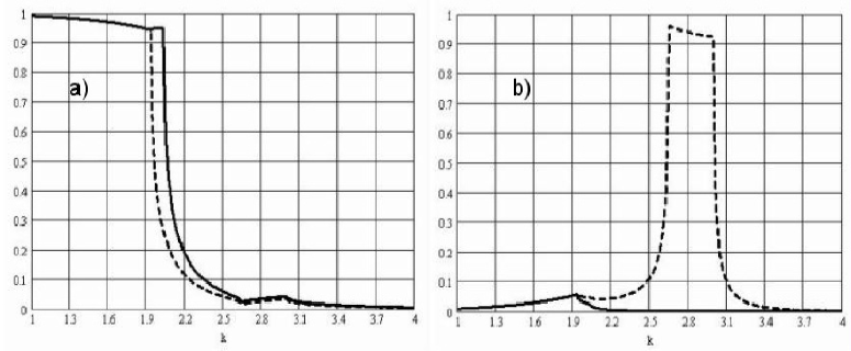
Figure 1: Dependence on wave number $k$ of reflectivities a) without and b) with spin flip. The solid curves are for initial polarization along $x$-axis, and the dashed curves are for the initial polarization along $-x$. Calculations were made for parameters $\mbox{${\rm\bf B}$}_{0}=0$, $u_{0}=4-0.01i$, $b=0.5$, $B=0.1$, $q=2$.

The most striking feature of the Fig. 1b), is the presence of a resonant peak with the center at the point $k=\sqrt{q^{2}+u_{0}}$ and the width determined by the field $\sqrt{b^{2}+B^{2}}$. The peak corresponds to almost total reflection with spin-flip, and it exists only for polarization of the incident neutron against the vector $q$, which characterizes the rotation of the field in the mirror.

Figure 2: Dependence on wave number $k$ of reflectivities a) without and b) with spin flip. The solid curves are for initial polarization along $x$-axis, and dashed curves are for initial polarization along $-x$. Calculations were made for parameters $\mbox{${\rm\bf B}$}_{0}=0$, $u_{0}=4-0.01i$, $b=0.5$, $B=0$, $q=2$. We see that the center of the peak is at $k=\sqrt{u_{0}+q^{2}}$, and almost total reflection with spin-flip takes place in the range $\sqrt{u_{0}+q^{2}-2b}<k<\sqrt{u_{0}+q^{2}-2b}$.

It is interesting to compare the obtained results to the case $B=0$, when we can use the quadratic equation (24) instead of the cubic one (16). The results for the same parameters except $B=0$ are shown in Fig. 2. We see that the main difference is the presence of two limiting energies at $B\neq 0$ for non spin-flip reflectivities. If we are interested in some peculiarities of reflectivities due to field rotation, we can neglect $B$, then we get quadratic equation (24) instead of the cubic one (16), and calculations are facilitated. So, below we set $B=0$.

IV Reflection from a mirror of a finite thickness

To find the reflection coefficients from a finite mirror at $0<z<l$, we need to know reflection and transmission matrices at interfaces for a wave incident at the from inside the mirror. At the interface $z=0$ the wave function can be written as:

$$|\psi(z)\rangle=\Theta(z<0)\exp(-i\mbox{\boldmath$\hat{k}$}_{0}z)\mbox{\boldmath$\hat{t}$}^{\prime}|\xi_{0}\rangle+$$

$$+\Theta(z>0)\exp(-i\sigma_{x}qz)\left(\exp(-i[a+\overleftarrow{\mbox{\boldmath$p$}}_{\varphi}\mbox{\boldmath$\sigma$}]z)+\exp(i[a+\overrightarrow{\mbox{\boldmath$p$}}_{\varphi}\mbox{\boldmath$\sigma$}]z)\mbox{\boldmath$\hat{r}$}^{\prime}\right)|\xi(0)\rangle,$$ (35)

where $\overleftarrow{\mbox{\boldmath$p$}}_{\varphi}\mbox{\boldmath$\sigma$}$ is defined like in (29). Matching this wave function at $z=0$ gives:

$$\mbox{\boldmath$\hat{t}$}^{\prime}=[\mbox{\boldmath$\hat{k}$}_{0}+a+\overrightarrow{\mbox{\boldmath$p$}}^{\prime}_{\varphi}\mbox{\boldmath$\sigma$}]^{-1}[2a+\overrightarrow{\mbox{\boldmath$p$}}^{\prime}_{\varphi}\mbox{\boldmath$\sigma$}+\overleftarrow{\mbox{\boldmath$p$}}^{\prime}_{\varphi}\mbox{\boldmath$\sigma$}],$$ (36)

$$\mbox{\boldmath$\hat{r}$}^{\prime}=[\mbox{\boldmath$\hat{k}$}_{0}+a+\overrightarrow{\mbox{\boldmath$p$}}^{\prime}_{\varphi}\mbox{\boldmath$\sigma$}]^{-1}[a+\overleftarrow{\mbox{\boldmath$p$}}^{\prime}_{\varphi}\mbox{\boldmath$\sigma$}-\mbox{\boldmath$\hat{k}$}_{0}],$$ (37)

where $\overleftarrow{\mbox{\boldmath$p$}}^{\prime}_{\varphi}\mbox{\boldmath$\sigma$}=e^{-i\sigma_{x}\varphi}(\overleftarrow{p}_{y}\sigma_{y}+\overleftarrow{p}_{z}\sigma_{z})e^{i\sigma_{x}\varphi}$.

In order to obtain the reflection and transmission matrices at $z=l$ it is convenient to shift the origin $z=0$ to this point. As a result the wave function there becomes:

$$\Theta(z<0)\exp(-iq\sigma_{x}z)\bigg{[}\exp(-i[a+\overleftarrow{\mbox{\boldmath$p$}}_{\phi}\mbox{\boldmath$\sigma$}]z)\mbox{\boldmath$\hat{r}$}^{\prime\prime}+\exp(i[a+\overrightarrow{\mbox{\boldmath$p$}}_{\phi}\mbox{\boldmath$\sigma$}]z)\bigg{]}\xi_{0}+$$

$$+\Theta(z>0)\exp(i\mbox{\boldmath$\hat{k}$}_{0}z)\mbox{\boldmath$\hat{t}$}^{\prime\prime}\xi_{0},$$ (38)

and we must take into account that $\mbox{\boldmath$\hat{t}$}^{\prime\prime}\neq\mbox{\boldmath$\hat{t}$}^{\prime}$, $\mbox{\boldmath$\hat{r}$}^{\prime\prime}\neq\mbox{\boldmath$\hat{r}$}^{\prime}$ and that the mismatch phase $\phi$ is not equal to $\varphi$ at the entrance surface. Matching this wave function at the interface leads to:

$$\mbox{\boldmath$\hat{t}$}^{\prime\prime}=[\mbox{\boldmath$\hat{k}$}_{0}+a+\overleftarrow{\mbox{\boldmath$p$}}^{\prime}_{\phi}\mbox{\boldmath$\sigma$}]^{-1}[2a+\overleftarrow{\mbox{\boldmath$p$}}^{\prime}_{\phi}\mbox{\boldmath$\sigma$}+\overrightarrow{\mbox{\boldmath$p$}}^{\prime}_{\phi}\mbox{\boldmath$\sigma$}],$$ (39)

$$\mbox{\boldmath$\hat{r}$}^{\prime\prime}=[\mbox{\boldmath$\hat{k}$}_{0}+a+\overleftarrow{\mbox{\boldmath$p$}}^{\prime}_{\phi}\mbox{\boldmath$\sigma$}]^{-1}[a+\overrightarrow{\mbox{\boldmath$p$}}^{\prime}_{\phi}\mbox{\boldmath$\sigma$}-\mbox{\boldmath$\hat{k}$}_{0}].$$ (40)

At the point $z=-l$ near the entrance surface the reflected wave of (38) is equal to $\exp(iq\sigma_{x}l)\exp(i[a+\overleftarrow{\mbox{\boldmath$p$}}_{\phi}\mbox{\boldmath$\sigma$}]l)\mbox{\boldmath$\hat{r}$}^{\prime\prime}\xi_{0}$.

Now we are well equipped to calculate reflection from a slab of thickness $l$. To facilitate slightly the calculations, we accept interface $\varphi=0$ at the entrance. Then, at the exit interface we will have $\varphi=ql$. Let’s denote the wave incident from inside the matter upon the exit interface at $z=l$ as $\mbox{$\hat{\rm\bf X}$}\xi_{0}$. For $\hat{\rm\bf X}$ we can construct a self consistent equation:

$$\mbox{$\hat{\rm\bf X}$}=\exp(-iq\sigma_{x}l)\exp(i[a+\overrightarrow{\mbox{\boldmath$p$}}\mbox{\boldmath$\sigma$}]l)\mbox{\boldmath$\hat{t}$}+$$

$$+\exp(-iq\sigma_{x}l)\exp(i[a+\overrightarrow{\mbox{\boldmath$p$}}\mbox{\boldmath$\sigma$}]l)\mbox{\boldmath$\hat{r}$}^{\prime}\exp(iq\sigma_{x}l)\exp(i[a+\overleftarrow{\mbox{\boldmath$p$}}_{qL}\mbox{\boldmath$\sigma$}]l)\mbox{\boldmath$\hat{r}$}^{\prime\prime}\mbox{$\hat{\rm\bf X}$},$$ (41)

which has the following solution:

$$\mbox{$\hat{\rm\bf X}$}=\bigg{[}I-\exp(-iq\sigma_{x}l)\exp(i[a+\overrightarrow{\mbox{\boldmath$p$}}\mbox{\boldmath$\sigma$}]l)\mbox{\boldmath$\hat{r}$}^{\prime}\exp(iq\sigma_{x}l)\exp(i[a+\overleftarrow{\mbox{\boldmath$p$}}_{q}\mbox{\boldmath$\sigma$}]L)\mbox{\boldmath$\hat{r}$}^{\prime\prime}\bigg{]}^{-1}\times$$

$$\times\exp(-iq\sigma_{x}l)\exp(i[a+\overrightarrow{\mbox{\boldmath$p$}}\mbox{\boldmath$\sigma$}]l)\mbox{\boldmath$\hat{t}$},$$ (42)

where $I$ is the unit matrix. With the help of $\hat{\rm\bf X}$ we can easily find the reflection, $\hat{\rm\bf R}$, and the transmission, $\hat{\rm\bf T}$, matrix amplitudes, which read:

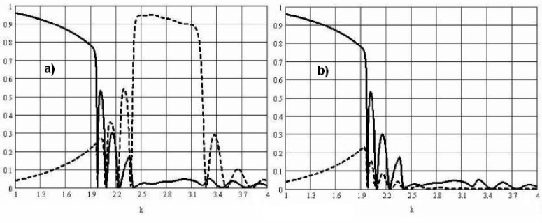
Figure 3: Dependence on $k$ of the reflectivities with (dashed curve) and without (solid curve) of the spin-flip from the mirror of thickness $l=8$ with fan-like magnetization. Initial polarization of the neutron is a) along $-x$, b) along $+x$. For calculations we used parameters $B_{0}=0$, $u_{0}=4-0.01i$, $q=2$, and $b=1$.

$${\rm{\bf\vec{R}}}={\rm{\bf\hat{r}}}+{\rm{\bf\hat{t}}}^{\prime}\exp\left({i\,q\sigma_{z}l}\right)\exp\left({i\,\left[{a+{\rm{\bf\mathord{\buildrel\lower 3.0pt\hbox{$\scriptscriptstyle\leftharpoonup$}\over{p}}}}_{qL}{\rm{\bf\sigma}}}\right]\,l}\right)\,\,{\rm{\bf\hat{r}}}^{{}^{\prime\prime}}{\rm{\bf\hat{{\rm X}}}},\quad{\rm{\bf\hat{T}}}={\rm{\bf\hat{t}}}^{{}^{\prime\prime}}{\rm{\bf\hat{{\rm X}}}}.$$ (43)

Using the analytical expressions (43) we can directly calculate matrix elements and find reflection and transmission probabilities with and without spin flip as a functions of $k$. The results of the calculations for $l=8$ and for the simplest case $B_{0}=0$ are shown in Fig. 3. Again, we clearly see the occurrence of the resonant peak. Its height decreases with decrease of $l$.

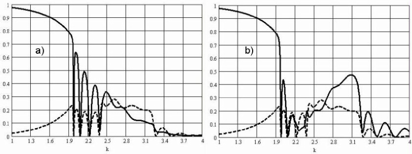
Figure 4: Dependence on $k$ of the reflectivities with (dashed curve) and without (solid curve) of the spin-flip from the mirror with fan-like magnetization in the external field $B_{0}=0.1$ parallel to the $y$-axis. Initial polarization of the neutron is a) opposite to $\mbox{${\rm\bf B}$}_{0}$, b) along it. Parameters $u_{0}$, $q$, $l$ and $b$ are the same as in Fig. 3. The mismatch phase $\varphi$ at the entrance surface is zero.

V Reflectivities for $\mbox{${\rm\bf B}$}_{0}\neq 0$

When the magnetic induction $\mbox{${\rm\bf B}$}_{0}\neq 0$, the quantization axis is to be chosen along $\mbox{${\rm\bf B}$}_{0}$. If $\mbox{${\rm\bf B}$}_{0}$ is parallel oriented with respect to the $y$-axis, then the incident neutron has a polarization $|\xi_{\pm y}\rangle$, which is a superposition of two opposite polarizations $|\xi_{\pm x}\rangle$:

$$\left|{\xi_{\pm y}}\right\rangle=\frac{1\pm i}{2}\left|{\xi_{+x}}\right\rangle+\frac{1\mp i}{2}\left|{\xi_{-x}}\right\rangle.$$ (44)

Therefore, the reflection amplitudes with spin flip, $R_{\pm\mp y}$, and without spin-flip $R_{\mp\mp y}$ contain contributions of the resonant amplitude $R_{+-x}$. This is clearly seen in Fig. 4. The results of the calculations for a mismatch phase $\varphi=0$ at the entrance surface show that the amplitudes with spin-flip are equal for both initial polarizations, and that the reflection amplitudes without spin-flip also contain a resonant peak at $\sqrt{u_{0}+q^{2}-2b}\leq k\leq\sqrt{u_{0}+q^{2}+2b}$.

For a real magnetic system dono , the values of the parameters are about: $q\approx 1$, $ql<\pi$ and $\mbox{$\varphi$}\neq 0$. The mismatch phase $\varphi$ depends on strength of the field $B_{0}$ and can be found from reflectivities curves.

VI Reflection from composition of soft and hard magnetics

Above we have considered the reflection from an abstract fan-like magnetic system. In reality, a fan-like magnetization state can appear in a SL which is magnetically coupled to a HL. In the following we assume that the HL of thickness $l_{h}$ with optical potential $u_{h}$ has an uniform magnetization ${\rm\bf b}$, which coincides with the magnetization of the SL at the exit interface $z=l$. The total reflection matrix amplitude $\mbox{\boldmath${\rm\bf R}$}_{sh}$ for the two magnetic layers and from the side of the soft one is  goto ; dono :

$$\mbox{\boldmath${\rm\bf R}$}_{sh}=\overrightarrow{\mbox{\boldmath${\rm\bf R}$}}+\overleftarrow{\mbox{\boldmath${\rm\bf T}$}}\mbox{\boldmath${\rm\bf R}$}_{h}[\mbox{\boldmath$\rm\bf I$}-\overleftarrow{\mbox{\boldmath${\rm\bf R}$}}\mbox{\boldmath${\rm\bf R}$}_{h}]^{-1}\overrightarrow{\mbox{\boldmath${\rm\bf T}$}},$$ (45)

and from the side of the hard one is:

$$\mbox{\boldmath${\rm\bf R}$}_{hs}=\mbox{\boldmath${\rm\bf R}$}_{h}+\mbox{\boldmath${\rm\bf T}$}_{h}\overleftarrow{\mbox{\boldmath${\rm\bf R}$}}_{h}[\mbox{\boldmath$\rm\bf I$}-\overleftarrow{\mbox{\boldmath${\rm\bf R}$}}\mbox{\boldmath${\rm\bf R}$}_{h}]^{-1}\mbox{\boldmath${\rm\bf T}$}_{h},$$ (46)

where $\mbox{\boldmath${\rm\bf R}$}_{h}$ and $\mbox{\boldmath${\rm\bf T}$}_{h}$ are the reflection and transmission matrices of the separate HL with vacuum and for the same external field on both sides of it:

$${\rm{\bf R}}_{h}={\rm{\bf r}}_{h}-({\rm{\bf I}}-{\rm{\bf r}}_{h})\exp(i{\rm{\bf k}}_{h}l_{h}){\rm{\bf r}}_{h}[\mbox{\boldmath$\rm\bf I$}-\exp(i{\rm{\bf k}}_{h}l_{h}){\rm{\bf r}}_{h}\exp(i{\rm{\bf k}}_{h}l_{h}){\rm{\bf r}}_{h}]^{-1}\exp(i{\rm{\bf k}}_{h}l_{h})({\rm{\bf I}}+{\rm{\bf r}}_{h}),$$ (47)

$$\mbox{\boldmath${\rm\bf T}$}_{h}=({\rm{\bf I}}-{\rm{\bf r}}_{h})[\mbox{\boldmath$\rm\bf I$}-\exp(i{\rm{\bf k}}_{h}l_{h}){\rm{\bf r}}_{h}\exp(i{\rm{\bf k}}_{h}l_{h}){\rm{\bf r}}_{h}]^{-1}\exp(i{\rm{\bf k}}_{h}l_{h})({\rm{\bf I}}+{\rm{\bf r}}_{h}),$$ (48)

${\rm{\bf k}}_{h}=\sqrt{k^{2}-u_{h}-2{\rm{\bf b}}_{h}{\rm{\bf\mbox{\boldmath$\sigma$}}}}$, and ${\rm{\bf r}}_{h}=({\rm{\bf k}}_{h}+{\rm{\bf k}}_{0})^{-1}({\rm{\bf k}}_{0}-{\rm{\bf k}}_{h})$ is the matrix reflection amplitude of the interface between the HL and vacuum.

The results of the calculations for $u_{h}=3.5-0.01i$ and $l_{h}=1.1$ are shown in Fig. 6. The top panels show reflectivities from the SL side a) without and b) with spin-flip, and the bottom panels show the analogous reflectivities from the HL side. The top and bottom figures are different. The resonance peak seen on the top figures, is replaced with the second total reflection edge when reflection is from the HL side. This is in good agreement with measured reflection curves dono . When the external field changes, the shapes of the top and bottom curves also change.

The results obtained by analytical methods were checked by numerical simulations with the generalized matrix method rad ; polar . Both types of calculations are in good agreement. For the numerical calculation, the SL was subdivided into 50 sub-layers with different directions of magnetization. The angular increment between two neighboring sub-layers was constant.

By making use of the numerical method, it is also possible to calculate reflectivities when rotation of the field is not uniform, and we can expect that nonuniform rotation will lead to broadening of the resonant peak and to a lowering of its height.

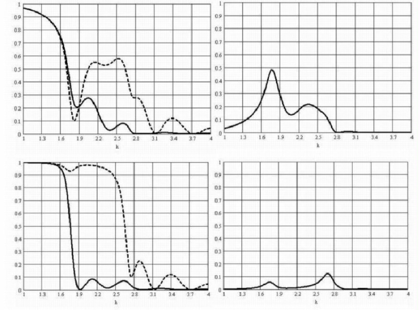
Figure 5: Dependence on $k$ of the reflectivities from (top) the SL side (bottom) from HL side. On the left panels the reflectivities without spin flip when initial polarization is against field $\mbox{${\rm\bf B}$}_{0}$ (solid curve) and along it (dashed curve) are shown. On the right panels the spin-flip reflectivities are shown. They are the same for both polarizations, therefore only one curve is plotted. For the calculations the following parameters have been used: $B_{0}=0.2$, $\varphi=0.1$, $u_{0}=4-0.0001i$, $b=1$, $q=1$, $l=3$, $u_{h}=3.5-0.001i$ and $l_{h}=1.1$.

VII Violation of some fundamental principles in the considered model

The resonant spin flip reflection from samples with rotating field (see also aks ) shows some features, which are very important with respect to fundamental principles. Reflectivity and transmissivity of samples with a field rotating around a $q$ vector contain a T-odd correlation $s$$q$, where $s$ is the incident neutron spin polarization. It looks as if there is a violation of the time reverse invariance. However more detailed considerations ifn show that the operator of the time reverse applied to the spinor wave function, containing T-odd terms, gives a new wave function, which is an exact solution of the time reversed Hamiltonian even in presence of absorption (imaginary part of the Hamiltonian). It proves that the T-invariance is not violated notwithstanding that the wave function contains the T-odd correlation. This example, however is very useful. It shows that observation in an experiment of T-odd or P-odd correlations should not be accepted as a proof of violation of P- or T-invariance.

In our problem we meet also violation of the detailed balance principle, related to the principle of maximal entropy. According to this principle the flux reflected with spin flip from the initial state $|\xi_{-x}\rangle$ is to be equal to the flux reflected with spin flip from the initial state $|\xi_{+x}\rangle$. Such equality is necessary because, if the mirror would be immersed in an isotropic distribution of unpolarized neutrons, the reflectivity would neither change the isotropy nor create polarization. In the case of the mirror with a rotating field it is not so. The neutrons in the state $|\xi_{-x}\rangle$ are reflected almost totally with spin flip, while the oppositely polarized neutrons are not reflected. It seems that, if we take a vessel with isotropic unpolarized neutron gas and partition it off by a magnetized foil with a rotating magnetization (helicoidal, fan-like or some other) then the neutrons from, say, the left part of the vessel will spill completely polarized through the foil into the right part of the vessel. Indeed the neutrons in the left part, which are polarized along $-x$, after reflection become polarized along $+x$ and these neutrons are easily transmitted without depolarization into the right side. So all the neutrons will go to the right side and they will be polarized along $+x$.

However such a terrible violation of the maximal entropy principle does not happen, because for neutrons on the right side of the foil the field in the foil looks rotating in the opposite direction, therefore the states $|\xi_{+x}\rangle$ are reflected almost totally with spin flip, and the states $|\xi_{-x}\rangle$ are easily transmitted to the left side. Nevertheless there appears a cycle in the phase space, which violates principle of the detailed balance. This violation is attributed to presence of rotation in space. If there were two opposite rotations the space could be considered having an equilibrium state, and the detailed balance would be not violated, With a single hand rotation the space is not in the equilibrium, and because of that the detailed balance is violated.

VIII Conclusion

We have obtained analytical expressions for calculation of reflectivities and transmissivity of neutrons through magnetic media with fan-like and helicoidal magnetization. The calculations show that at wave numbers in the interval $\sqrt{u_{0}+q^{2}-2b}<k<\sqrt{u_{0}+q^{2}+2b}$, where $q$ is the fan vector (rotation vector of the fan), and $b$ is the internal magnetic field of the fan, the reflection curve contains a resonance peak. This feature serves as an identification of magnetic configurations with intrinsic rotating fields. The width of the peak characterizes the uniformity of rotation and the strength of the rotating field. The analytical solutions and the numerical generalized matrix method are very useful tools for analyzing polarized neutron reflectivity data from non-collinear magnets exhibiting anisotropic exchange forces.

The time parity violation found in this model shows that observation of such an effect in some experiment must be analyzed in order to exclude the presence of magnetic fields, which may rotate in the sample space.

References

• (1) J. B. Kortright, M. Rice, S.-K. Kim, C.C. Walton, T. Warwick, Magn. Magn. Mater. 207, 7-44, (1999).
• (2) A. I. Buzdin, Rev. Mod. Phys. 77 935-976 (2005).
• (3) C. Leighton, M. R. Fitzsimmons, P. Yashar, A. Hoffmann, J. Nogués, J. Dura, C. F. Majkrzak, and Ivan K. Schuller, Phys. Rev. Lett. 86, 4394 (2001); M. R. Fitzsimmons, P. Yashar, C. Leighton, Ivan K. Schuller, J. Nogués, C. F. Majkrzak, and J. A. Dura, Phys. Rev. Lett. 84, 3986 (2000).
• (4) M.Calvo, Phys. Rev. B 18, 5073 (1978).
• (5) E. Goto, N. Hayashi, T. Miyashita, and K. Nakagawa, J. Appl. Phys. 36, 2951 (1965).
• (6) K. V. O’Donovan, J. A. Borchers, C. F. Majkrzak, O. Hellwig, and E. E. Fullerton, Phys. Rev. Lett. 88, 067201 (2002)
• (7) V. E. Kuncser, M. Doi, W. Keune, M. Askin, H. Spies, J. S. Jiang, A. Inomata, and S. D. Bader, Phys. Rev. B 68, 064416 (2003).
• (8) O. Hellwig, J. B. Kortright, K. Takano, and Eric E. Fullerton, Phys. Rev. B 62, 11694 (2003).
• (9) G. Asti, M. Ghidini, R. Pellicelli, C. Pernechele, M. Solzi, F. Albertini, F. Casoli, S. Fabbrici, and L. Pareti. Magnetic phase diagram and demagnetization processes in perpendicular exchange-spring multilayers. Phys.Rev. B 73, 094406, (2006).
• (10) R. H. Victora, and Xiao Shen. Composite Media for Perpendicular Magnetic Recording. IEEE Trans.Magn. 41, 537-42, (2005).
• (11) V. L. Aksenov, V. K. Ignatovich, Yu. V. Nikitenko, Crystallography Reports 51, 734-753 (2006).
• (12) F. Radu, V. K. Ignatovich, Physica B 267-268, 175-180 (1999).
• (13) F. Radu. Polarized Neutron Reflectometry Software “POLAR”
http://www.ep4.rub.de/radu/welcome/polar.html.
• (14) A. Ruhm, B. P. Toperverg, and H. Dosch, Phys. Rev. B 60, 16073 (1999).
• (15) L. Deak, L. Bottyan, D. L. Nagy, and H. Spiering, Physica B 297 , 113 (2001).
• (16) V.K.Ignatovich, Yu.V.Nikitenko. T-odd correlations in neutron reflectometry experiments. Proc. XVII International seminar on Interaction of Neutrons with Nuclei, Dubna May 27-30 2009. To be published. arXiv:0906.2684v2 [quant-ph]: http://arxiv.org/abs/0906.2684