Hypertractions and hyperstresses convey the same mechanical information

Abstract

A strengthened and generalized version of the standard Virtual Work Principle is shown to imply, in addition to bulk and boundary balances, a one-to-one correspondence between surface and edge hypertractions and hyperstrestress fields in second-grade continua. When edge hypertractions are constitutively taken null, the hyperstress is shown to take the form it has for a Navier-Stokes$-\alpha$ fluid, a relevant example of second-grade fluid-like material.

1 Introduction

The main conceptual point we want to make in this note is that stipulating a suitable Principle of Virtual Powers to characterize mechanical equilibrium of continua of any grade bigger than one offers a key advantage: a Cauchy-type construction of the hyperstress fields accompanying the equilibrium hypertraction fields (a difficult task, that has been undertaken but not achieved so far) is no more needed, because hyperstresses can be explicitly computed in terms of hypertractions, and conversely. In this paper, we demonstrate this tenet in the case of second-gradient continua, by a simple argument.

Theories of second-gradient continua have a long history. In the case of fluids, a possible dependence of pressure on the density gradient was first proposed by Korteweg [9] to model capillarity effects in 1901; for solids, two pioneering papers by Toupin [15, 16] on elastic materials with couple stresses appeared in the early years 1960. A PVP approach to the formulation of the basic balance laws for these continua was taken by Germain [5, 6, 7] in the early 1970s; the comprehensive article by Maugin [10] appeared in 1980; a recent contribution, of special relevance to our present paper, is due to Gurtin and Fried [4].

It is well known that compatibility with the second law of thermodynamics for constitutive relations which are functions of the second deformation gradient demands that internal mechanical interactions have a nonstandard form. This has been discussed by many authors, mainly with an eye towards a better clarification of the role of the so-called hypertractions and hyperstresses; an important contribution was given by Dunn and Serrin [2], who introduced the notion of the interstitial energy. An interesting feature of second-gradient materials is that, if bodies and subbodies having non everywhere smooth boundary are considered, then edge forces, that is, line distributions of hypertractions are to be expected (and, if a dependence on gradients higher than two is allowed, one has to deal also with vertex forces, as exemplified by Podio-Guidugli [12]). To our knowledge, a rigorous interaction theory accommodating such a nonstandard behavior remains to be constructed; interesting attempts in this direction have been carried out by Forte and Vianello [3], Noll and Virga [11], and Dell’Isola and Seppecher [1].

Although here we do not deal with this difficult issue directly, in Section 3, the bulk of this paper, we do provide a full set of representation formulae not only, as is relatively easy, for tractions and hypertractions, both diffused and concentrated on edges, in terms of stresses and hyperstresses (see definitions (46)₁, (46)₂, and (47)) but also, conversely, for stresses and hyperstresses in terms of diffused and concentrated tractions and hypertractions (see (48)-(49), and (60)). Such representation formulae generalize the corresponding formulae for simple ($\equiv$ first-gradient) materials, that we derive in our preparatory Section 2. Since we work in a nonvariational setting, our results apply whatever the material response. The PVP we use includes edge tractions, both internal and external; without them, it would not be possible to arrive at the complete representation formula for the hyperstress in terms of hypertractions we construct in Subsection 3.5.

Finally, in Section 4, we provide a new proof of the following not very well-known fact in the theory of second-gradient materials: if edge tractions are constitutively presumed null on whatever edge, then the hyperstress needs not be zero, although it takes a very special form whose information content is carried by a vector field. We surmise that inability to develop edge interactions be characteristic of certain second-gradient fluids, an issue that we take up in a forthcoming paper [14], continuing a line of thought proposed in [13].

2 Simple Continua

2.1 Power expenditures as constitutive requirements

When a characterization of mechanical equilibrium is sought via a weak formulation of the virtual-work type, the primary object is a linear space $\mathcal{V}$ of test($\equiv\,$virtual) velocity fields; the collection of tractions is introduced as the formal dual of $\mathcal{V}$, by laying down a notion of external power expended in a virtual body motion; and the collection of stresses is introduced as the formal dual of the collection of test-velocity gradients, by laying down a notion of internal power. We regard specification of these two duality relations as the ‘zeroth grade’ of any constitutive theory.

We classify a material body $B$ as simple if the internal and external power expenditures have the following forms:

$${\mathcal{W}}^{(i)}(P)[\mathbf{v}] :=\int_{P}\mathbf{T}\cdot\operatorname{grad}\mathbf{v},$$ (1)

$${\mathcal{W}}^{(e)}(P)[\mathbf{v}] :=\int_{\partial P}\mathbf{t}\cdot\mathbf{v}\,,$$

for all body parts($\equiv\,$subbodies) $P$ and for all test-velocity fields $\mathbf{v}\in{\mathcal{V}}$. Here $P$ is a bounded subset of the current observation space being regularly open (that is, coinciding with the interior of its closure) and having a part-wise regular boundary $\partial P$; we regard it as the region occupied by the typical body part at the time of our observation; time itself plays the role of a parameter. As to $\mathcal{V}$, we accept the standard assumption that it includes all realizable velocities (that is, all velocity fields obtained by time differentiation of admissible deformation fields) and that it is closed under the operation ${\mathcal{O}}$ of observer change, in the sense that, if $\mathbf{v}\in{\mathcal{V}}$, then

$$\mathbf{v}^{+}={\mathcal{O}}(\mathbf{v})=\dot{}\mathbf{q}+\mathbf{Q}\mathbf{v}+\mathbf{W}\mathbf{x}^{+}\in{\mathcal{V}}$$ (2)

for all translation velocities $\dot{}\mathbf{q}$, all rotations ($\equiv$ proper orthogonal tensors) $\mathbf{Q}$, and all relative spins ($\equiv$ skew-symmetric tensors) $\mathbf{W}$ (for details, see the first subsection of the Appendix).

The internal field $\mathbf{T}$, the Cauchy stress, is meant to measure the mechanical interaction of a material element of the subbody $P$ with its immediate adjacencies; the external field $\mathbf{t}$, the contact traction, is meant to account for the mechanical action exerted on $P$ by its complement with respect to the material universe the body $B$ belongs to. (We intentionally ignore all types of actions at a distance, because they are inessential to the purpose of our present discussion.)

Both fields $\mathbf{T}$ and $\mathbf{t}$ are here introduced formally by way of Riesz duality with, respectively, the test velocity fields $\mathbf{v}$ and their gradient fields $\operatorname{grad}\mathbf{v}$. Both power expenditures $\mathbf{T}\cdot\operatorname{grad}\mathbf{v}$ and $\mathbf{t}\cdot\mathbf{v}$ are required to be properly invariant under observer changes. Precisely, translational invariance of the external power expenditure over an arbitrary subbody implies that the contact traction field be balanced, i.e., that

$$\int_{\partial P}\mathbf{t}={\mathbf{0}}\quad\mbox{for all subbodies $P$.}$$ (3)

Moreover, the specific external power expenditure is rotationally invariant if and only if the contact traction is indifferent to observer changes, in the sense that

$${\mathcal{O}}(\mathbf{t})=\mathbf{t}^{+}=\mathbf{Q}\mathbf{t}\quad\mbox{for all rotations $\mathbf{Q}$}.$$ (4)

As to the specific internal power expenditure, which is quickly seen to be invariant under translational observer changes, its rotational invariance implies that, at all points of $B$, the Cauchy stress field be symmetric-valued and indifferent to observer changes, in the sense that

$${\mathcal{O}}(\mathbf{T})=\mathbf{T}^{+}=\mathbf{Q}\mathbf{T}\mathbf{Q}^{T}$$ (5)

(for a proof of this result, see the Appendix).

2.2 Mutual consistency of stresses and tractions via a strengthened Principle of Virtual Powers

The mutual consistency of the stress and traction fields is the consequence of postulating the following Principle of Virtual Power:

$${\mathcal{W}}^{(i)}(P)[\mathbf{v}]={\mathcal{W}}^{(e)}(P)[\mathbf{v}],$$ (6)

for all body parts $P$ and for all test-velocity fields $\mathbf{v}$.

Needless to say, the Principle is an invariant statement. The quantification on velocities is standard, that on body parts is not. Asking that (6) holds for all body parts is much stronger a requirement than demanding it to hold only for the whole body. This additional strength connects the values taken by $\mathbf{T}$ and $\mathbf{t}$ at all points of $B$, and not only at its boundary points.

With the use of a standard integration-by-parts lemma, we find that

$$\int_{P}\mathbf{T}\cdot\operatorname{grad}\mathbf{v}=\int_{P}(-\operatorname{div}\mathbf{T})\cdot\mathbf{v}+\int_{\partial P}\mathbf{T}\mathbf{n}\cdot\mathbf{v}.$$ (7)

Consequently, (6) can be written as follows:

$$\int_{P}(-\operatorname{div}\mathbf{T})\cdot\mathbf{v}+\int_{\partial P}\mathbf{T}\mathbf{n}\cdot\mathbf{v}=\int_{\partial P}\mathbf{t}\cdot\mathbf{v},$$ (8)

for all body parts $P$ and for all test velocity fields $\mathbf{v}$; in particular,

$$\int_{B}(-\operatorname{div}\mathbf{T})\cdot\mathbf{v}+\int_{\partial B}\mathbf{T}\mathbf{n}\cdot\mathbf{v}=\int_{\partial B}\mathbf{t}\cdot\mathbf{v},$$ (9)

for all test velocity fields $\mathbf{v}$. Now, while both (8) and (9) imply the classic pointwise balance:

$$-\operatorname{div}\mathbf{T}={\mathbf{0}}\quad\mbox{at all points of $B$,}$$ (10)

it is (8) that implies that

$$\mathbf{T}\mathbf{n}=\mathbf{t}\quad\mbox{at all points of $B$ and for all unit vectors $\mathbf{n}$,}$$ (11)

and not only at the points of $\partial B$ and for $\mathbf{n}$ the outward unit normal field, as implied by the weaker statement (9).

A first direct consequence of (11) is that

$$\mathbf{t}=\hat{}\mathbf{t}(x,\mathbf{n}),$$ (12)

namely, that – within the class of simple continua – the traction field at any point $x\in B$ must be thought of as depending on the orientation of the plane chosen through that point in order to detect the mutual mechanical contact interactions. Secondly, it follows from (11) that the fields $\mathbf{T}$ and $\mathbf{t}$ carry essentially the same information. Indeed, while, given the Cauchy stress mapping $x\mapsto\hat{}\mathbf{T}(x)$, (11) yields that

$$\hat{}\mathbf{t}(x,\mathbf{n})=\hat{}\mathbf{T}(x)\mathbf{n},$$ (13)

we also have that, given the traction mapping $(x,\mathbf{n})\mapsto\hat{}\mathbf{t}(x,\mathbf{n})$, the Cauchy stress field can be constructed as follows:

$$\hat{}\mathbf{T}(x)=\sum_{i}\hat{}\mathbf{t}(x,\mathbf{n}^{(i)})\otimes\mathbf{n}^{(i)},$$ (14)

for $\mathbf{n}^{(i)}\;(i=1,2,3)$ any three mutually orthogonal directions. Thus, (11) can be regarded as a basic consistency condition for the pair of dynamic quantities $(\mathbf{t},\mathbf{T})$ dual to the kinematic quantities $(\mathbf{v},\operatorname{grad}\mathbf{v})$, a condition that yields the representation formulae (13) and (14).

All these results are more or less well known in the continuum mechanics community. The main reason for us to recapitulate them is that they prompt the following remarks, that are at the core of our present work.

2.3 Thinking of complex continua

Relations (13) and (14) are also arrived at when, as is customary, only tractions on body parts are introduced, because stress is constructed à la Cauchy as a consequence of balance of tetrahedron-shaped parts. The Cauchy construction is the pillar on top of which the standard theory of diffuse (i.e., absolutely continuous with respect to the area measure) contact interactions stands. For complex (i.e., nonsimple) material bodies, a Cauchy-like construction has been attempted often, but not achieved so far, to our knowledge. Consequently, for such continua, although there is some sort of a general agreement about what notion of diffuse contact interactions applies, it is not clear what generalized stresses should accompany them to achieve mechanical balance. Now, as we just showed for simple material bodies acted upon by diffuse contact interactions, a key advantage of a Principle of Virtual Power quantified over a large collection of body parts is that it dispenses us from going through Cauchy’s tetrahedron construction to represent stress in terms of tractions. In the next section, this feature of a virtual-power approach to formulate mechanical balance is demonstrated in the case of a popular type of complex continua: we show what consistency relations restrict the choices of tractions/hypertractions and stresses/hyperstresses, and we derive representation formulae that generalize relations (13) and (14), where edge hypertractions have a crucial role.

3 Second-Gradient Continua

3.1 Notation

$\mathsf{H}$, a capital letter from a sansserif font, is used to denote the third-order hyperstress tensor. We write $H_{ijk}$ for the cartesian components of $\mathsf{H}$ with respect to a fixed orthonormal basis ${\mathbf{e}}_{i}$. For any vector $\mathbf{a}$, we write $\mathsf{H}\mathbf{a}$ for the second-order tensor with components $(\mathsf{H}\mathbf{a})_{ij}=H_{ijk}a_{k}$ (summation over repeated indexes understood); and, for any second-order tensor $\mathbf{A}$, we write $\mathsf{H}[\mathbf{A}]$ for the vector whose cartesian components are $(\mathsf{H}[\mathbf{A}])_{i}=H_{ijk}A_{jk}$; in particular, $\mathsf{H}[\mathbf{a}\otimes\mathbf{b}]=(\mathsf{H}\mathbf{b})\mathbf{a}$.

Let $\mathcal{V}$ be the translation space associated to the euclidean space where $\mathcal{S}$, a smooth surface, is embedded. Given any point of $\mathcal{S}$, we denote by ${}^{s}\mathbf{P}$ the orthogonal projection of the vector space $\mathcal{V}$ onto the tangent space to $\mathcal{S}$ at that point. The transpose of ${}^{s}\mathbf{P}$ is ${}^{s}\mathbf{I}$, the inclusion map, which takes any vector in the tangent space into a vector of $\mathcal{V}$. Thus, for $\mathbf{n}$ a unit normal to the surface and $\mathbf{I}$ the identity mapping over $\mathcal{V}$, ${}^{s}\mathbf{I}{}^{s}\mathbf{P}=\mathbf{I}-\mathbf{n}\otimes\mathbf{n}$.

3.2 Virtual power expenditures

Among complex material bodies, second-gradient continua are those for which the internal and external power expenditures have the following forms:

• (internal power expenditure)

  $${\mathcal{W}}^{(i)}(P)[\mathbf{v}]:=\int_{P}\mathbf{T}\cdot\operatorname{grad}\mathbf{v}+\mathsf{H}\cdot\operatorname{grad}\negthinspace^{2}\mathbf{v},$$ (15)

  where $\operatorname{grad}\negthinspace^{2}\,\mathbf{v}:=\operatorname{grad}(\operatorname{grad}\mathbf{v})$ is the second spatial gradient of the velocity field, and $\mathsf{H}$ is a third-order tensor field which satisfies:

  $$(\mathsf{H}\mathbf{a})\mathbf{b}=(\mathsf{H}\mathbf{b})\mathbf{a},\quad\textrm{for all vectors $\mathbf{a},\mathbf{b}$},$$ (16)

  so as to have the same index symmetries as the field $\operatorname{grad}\negthinspace^{2}\,\mathbf{v}$ it is dual to;

• (external power expenditure)

  $${\mathcal{W}}^{(e)}(P)[\mathbf{v}]:=\int_{\partial P}\big{(}\mathbf{t}\cdot\mathbf{v}+\mathbf{h}\cdot\partial_{\mathbf{n}}\mathbf{v}\big{)}+\int_{\widehat{\partial P}}\mathbf{f}\,^{\mathrm{e}}\cdot\mathbf{v}\,,$$ (17)

  where $\widehat{\partial P}$ is the ‘edgy’ part of $\partial P$, if any (once again, and for the same reasons as before, any distance interaction entering the external power has been ignored).

These definitions require some comments. Firstly, we here consider a part collection larger than usual: the boundary $\partial P$ of a part may happen to be the union of a finite number of regular surfaces which join pairwise along edges, that is, smooth curves which begin and end at singular points called vertices; accordingly, the edgy part $\widehat{\partial P}$ of $\partial P$ is the union of a finite set of boundary curves where the surface-normal field has a jump. Secondly, the introduction in (15) of the additional internal power expenditure associated with the hyperstress $\mathsf{H}$ is paraleled by the introduction in (17) of two types of external power expenditures associated with hypertractions, both additional to the one associated with the traction field $\mathbf{t}$, namely, the diffused hypertraction field $\mathbf{h}$ and the edge-force field $\mathbf{f}\,^{\mathrm{e}}$. Thirdly, the consequences of requiring that both power expenditures be properly invariant under observer changes must be investigated. We treat the two last issues in the following subsections.

3.2.1 Diffused and concentrated hypertractions

Suppose that, for consistency with postulating an additional power expenditure in the bulk associated with the second velocity gradient, one associates with the first the following additional power expenditure at a part’s boundary:

$$\int_{\partial P}\mathbf{H}\cdot\operatorname{grad}\mathbf{v},$$ (18)

with $\mathbf{H}$ some second-order tensor field work-conjugated to $\operatorname{grad}\mathbf{v}$. Then, on splitting the velocity gradient into its tangential and normal parts:

$$\operatorname{grad}\mathbf{v}=({}^{s}\negmedspace\operatorname{grad}\mathbf{v}){}^{s}\mathbf{P}+\partial_{\mathbf{n}}\mathbf{v}\otimes\mathbf{n},$$ (19)

we have that

$$\int_{\partial P}\mathbf{H}\cdot\operatorname{grad}\mathbf{v}=\int_{\partial P}(\mathbf{H}{}^{s}\mathbf{I})\cdot{}^{s}\negmedspace\operatorname{grad}\mathbf{v}+\int_{\partial P}\mathbf{H}\mathbf{n}\cdot\partial_{\mathbf{n}}\mathbf{v}\,.$$ (20)

Now, on setting $\mathbf{H}\mathbf{n}=\mathbf{h}$, the second integral on the right side of (20) can be identified with the second surface integral in (17); to motivate the presence of the line integral, we need a consequence of a surface-divergence identity, that we introduce right away.

Let $\mathcal{S}$ be a regular surface, oriented by its normal $\mathbf{n}$. At each point $\bm{x}$ of its boundary curve $\partial{\mathcal{S}}$, a unit vector $\mathbf{m}$ can be chosen, orthogonal to both $\mathbf{n}$ and the tangent direction of $\partial{\mathcal{S}}$ and pointing outward from the interior of $\mathcal{S}$; such a vector $\mathbf{m}$ lies in the limiting tangent plane to $\mathcal{S}$ at $\bm{x}$, and can be represented as $\mathbf{m}={}^{s}\mathbf{I}\bm{\mu}$, with $\bm{\mu}$ the appropriate tangent vector. For any smooth tensor field $\mathbf{A}$ over $\mathcal{S}$, the following integral identity holds true:

$$\int_{\mathcal{S}}(\mathbf{A}{}^{s}\mathbf{I})\cdot{}^{s}\negmedspace\operatorname{grad}\mathbf{v}=-\int_{\mathcal{S}}{}^{s}\negmedspace\operatorname{div}(\mathbf{A}{}^{s}\mathbf{I})\cdot\mathbf{v}+\int_{\partial{\mathcal{S}}}\mathbf{A}\mathbf{m}\cdot\mathbf{v}\,.$$ (21)

With a view to applying this identity to each regular portion of the boundary of an edgy body part, we draw attention to Figure 1,

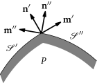
Figure 1: Four unit vectors describe an edge of a body part.

that depicts an edge cross-section of a part $P$. The limiting values of the outward unit normals to the surfaces $\mathcal{S}^{\prime}$ and $\mathcal{S}^{\prime\prime}$ joining at the edge are $\mathbf{n}^{\prime}$ and $\mathbf{n}^{\prime\prime}$, while the unit vectors $\mathbf{m}^{\prime}$ and $\mathbf{m}^{\prime\prime}$ belong to the tangent planes to those surfaces, and point outward from their interior. The edge $\mathcal{E}$ is described by an ordered list of four unit vectors:

$$\mathcal{E}\equiv(\mathbf{n}^{\prime},\mathbf{m}^{\prime};\mathbf{n}^{\prime\prime},\mathbf{m}^{\prime\prime})\,.$$ (22)

Note that the vectors in the list are not independent, because they are coplanar and pairwise orthogonal; moreover, the ordered pairs $(\mathbf{n}^{\prime},\mathbf{m}^{\prime})$ and $(\mathbf{n}^{\prime\prime},\mathbf{m}^{\prime\prime})$ can be interchanged freely. With the stipulated conventions, (22) gives a local (first-order) description of the geometry of an edge, just as a unit normal provides a local (first-order) description of an oriented surface.

With this notation, the identity (21) yields:

$$\int_{\partial P}(\mathbf{H}{}^{s}\mathbf{I})\cdot{}^{s}\negmedspace\operatorname{grad}\mathbf{v}=-\int_{\partial P}{}^{s}\negmedspace\operatorname{div}(\mathbf{H}{}^{s}\mathbf{I})\cdot\mathbf{v}+\int_{\widehat{\partial P}}\llbracket\mathbf{H}\mathbf{m}\rrbracket\cdot\mathbf{v},$$ (23)

where $\llbracket\mathbf{H}\mathbf{m}\rrbracket$ denotes twice the edge average of $\mathbf{H}\mathbf{m}$:

$$\llbracket\mathbf{H}\mathbf{m}\rrbracket:=\mathbf{H}\mathbf{m}^{\prime}+\mathbf{H}\mathbf{m}^{\prime\prime},$$ (24)

a vector field over $\widehat{\partial P}$. Thus, while the first in (23) can be safely thought as absorbed into the first surface integral in (17), the second motivates the introduction in (17) itself of the line integral over the edgy part of ${\partial P}$.

3.2.2 Invariance of power expenditures under observer changes

Translational and rotational invariances of the external power expenditure over an arbitrary subbody imply, respectively, the hypertraction balance

$$\int_{\partial P}\mathbf{t}\;+\int_{\widehat{\partial P}}\mathbf{f}\,^{\mathrm{e}}={\mathbf{0}}\quad\mbox{for all subbodies $P$.}$$ (25)

and the indifference properties

$$\mathbf{t}^{+}=\mathbf{Q}\mathbf{t},\quad\mathbf{h}^{+}=\mathbf{Q}\mathbf{h},\quad({\mathbf{f}\,^{\mathrm{e}}})^{+}=\mathbf{Q}\mathbf{f}\,^{\mathrm{e}}\quad\mbox{for all rotations $\mathbf{Q}$}.$$ (26)

It is shown in the Appendix that the rotational invariance of the specific internal power expenditure implies that, at all points of $B$, (i) the stress field $\mathbf{T}$ be symmetric-valued and indifferent to observer changes, just as it was the case for the Cauchy stress field in simple continua, and (ii) the hyperstress field $\mathsf{H}$ be indifferent to observer changes, in the sense that

$$\mathsf{H}^{+}=\mathbf{Q}\ast\mathsf{H},\quad\textrm{with}\;\;(\mathbf{Q}\ast\mathsf{H})[\mathbf{a}\otimes\mathbf{b}]\cdot\mathbf{c}=\mathsf{H}[\mathbf{Q}^{T}\mathbf{a}\otimes\mathbf{Q}^{T}\mathbf{b}]\cdot\mathbf{Q}^{T}\mathbf{c}\,.$$ (27)

3.3 The Principle of Virtual Powers and its consequences

We postulate the following Principle of Virtual Powers:

$${\mathcal{W}}^{(i)}(P)[\mathbf{v}]={\mathcal{W}}^{(e)}(P)[\mathbf{v}],$$ (28)

for all body parts $P$ and for all test velocity fields $\mathbf{v}$.

We want to show that there are two types of consequences of the part-wise balance principle (28):

• point-wise bulk and boundary balances, the same that would follow from a standard global Principle, stated for $P\equiv B$ only and quantified over the collection of test velocity fields;

• mutual consistency relations for the stress fields $(\mathbf{T},\mathsf{H})$ and the traction fields $(\mathbf{t},\mathbf{h},\mathbf{f}\,^{\mathrm{e}})$, such that either list determines uniquely the other, thus allowing the conclusion that each list conveys the same mechanical information.

We begin by noticing that, via repeated integration by parts, we have that

$${\int_{P}\mathbf{T}\cdot\operatorname{grad}\mathbf{v}+\mathsf{H}\cdot(\operatorname{grad}\negthinspace^{2}\mathbf{v})}={\int_{P}\big{(}\mathbf{T}-\operatorname{div}\mathsf{H})\cdot\operatorname{grad}\mathbf{v}+\int_{\partial P}\mathsf{H}\mathbf{n}\cdot\operatorname{grad}\mathbf{v}}$$ (29)

$$= {\int_{P}(-\operatorname{div}\widetilde{}\mathbf{T})\cdot\mathbf{v}+\int_{\partial P}}\big{(}\widetilde{}\mathbf{T}\mathbf{n}\cdot\mathbf{v}+(\mathsf{H}\mathbf{n})\mathbf{n}\cdot\partial_{\mathbf{n}}\mathbf{v}+(\mathsf{H}\mathbf{n})\cdot{}^{s}\negmedspace\operatorname{grad}\mathbf{v}\big{)},$$

where we have set

$$\widetilde{}\mathbf{T}:=\mathbf{T}-\operatorname{div}\mathsf{H}.$$ (30)

Next, just as we deduced (23) from (21), we find that

$$\int_{\partial P}(\mathsf{H}\mathbf{n})\cdot{}^{s}\negmedspace\operatorname{grad}\mathbf{v}=-\int_{\partial P}{}^{s}\negmedspace\operatorname{div}((\mathsf{H}\mathbf{n}){}^{s}\mathbf{I})\cdot\mathbf{v}+\int_{\widehat{\partial P}}\llbracket(\mathsf{H}\mathbf{n})\mathbf{m}\rrbracket\cdot\mathbf{v}.$$ (31)

Thus, the PVP relation (28) can be given the following provisional form:

$$\begin{gathered}\int_{P}(-\operatorname{div}\widetilde{}\mathbf{T})\cdot\mathbf{v}+\int_{\partial P}\Big{(}\big{(}\widetilde{}\mathbf{T}\mathbf{n}-{}^{s}\negmedspace\operatorname{div}((\mathsf{H}\mathbf{n}){}^{s}\mathbf{I})\big{)}\cdot\mathbf{v}+(\mathsf{H}\mathbf{n})\mathbf{n}\cdot\partial_{\mathbf{n}}\mathbf{v}\Big{)}\\ +\int_{\widehat{\partial P}}\llbracket(\mathsf{H}\mathbf{n})\mathbf{m}\rrbracket\cdot\mathbf{v}=\int_{\partial P}\big{(}\mathbf{t}\cdot\mathbf{v}+\mathbf{h}\cdot\partial_{\mathbf{n}}\mathbf{v}\big{)}+\int_{\widehat{\partial P}}\mathbf{f}\,^{\mathrm{e}}\cdot\mathbf{v}\,,\end{gathered}$$ (32)

for all subbodies and all virtual velocity fields.

By exploiting both quantifications with the use of smooth body parts only, we have from (32) that, at all points of $B$, the following balances must hold:

$$-\operatorname{div}\widetilde{}\mathbf{T}={\mathbf{0}},$$ (33)

with $\widetilde{}\mathbf{T}$ defined by (30) in terms of $\mathbf{T}$ and $\mathsf{H}$; moreover, for each unit vector $\mathbf{n}$,

$$\widetilde{}\mathbf{T}\mathbf{n}-{}^{s}\negmedspace\operatorname{div}((\mathsf{H}\mathbf{n}){}^{s}\mathbf{I})=\mathbf{t},\quad\textrm{for all smooth surfaces oriented by}\;\mathbf{n};$$ (34)

and

$$(\mathsf{H}\mathbf{n})\mathbf{n}=\mathbf{h}.$$ (35)

Notice that the last relation can also be written as

$$\mathsf{H}[\mathbf{n}\otimes\mathbf{n}]=\mathbf{h},\quad\textrm{for all unit vectors}\;\mathbf{n}.$$ (36)

The remain of (32) is

$$\int_{\widehat{\partial P}}\big{(}\llbracket(\mathsf{H}\mathbf{n})\mathbf{m}\rrbracket-\mathbf{f}\,^{\mathrm{e}}\big{)}\cdot\mathbf{v}=0\,,$$ (37)

for all edgy body parts and all test velocity fields. Consequently, we have that, again at all points of $B$,

$$\llbracket(\mathsf{H}\mathbf{n})\mathbf{m}\rrbracket=\mathbf{f}\,^{\mathrm{e}},\quad\textrm{for all edges}\;{\mathcal{E}},$$ (38)

or rather, more explicitly,

$$\mathsf{H}[\mathbf{n}^{\prime}\otimes\mathbf{m}^{\prime}+\mathbf{n}^{\prime\prime}\otimes\mathbf{m}^{\prime\prime}]=\mathbf{f}\,^{\mathrm{e}},\quad\textrm{for all edges as in Figure~{}\ref{fig:generic.edge}}.$$ (39)

Remark. Differences in notation apart, equations (33), (34)-(35) and (38) coincide respectively with equations (4), (5) and (49) of Gurtin and Fried [4]; as they remark, when applied to the body’s boundary, those equations are the same as equations (7.8), (7.9) and (7.10), derived variationally by Toupin in [15]. Our equation (34), however, is written in much more compact a form than the corresponding equations in [4] and [15]. Interestingly, as noticed earlier by Forte and Vianello [3], this opens the way to a suggestive analogy with

$$\mathbf{F}\mathbf{n}-{}^{s}\negmedspace\operatorname{div}\mathbf{M}=\mathbf{t},$$ (40)

the balance equation in shell theory that involves the force and moment tensors $\mathbf{F}$ and $\mathbf{M}$, that is, the surface-stress descriptors of that theory; the following identifications suffice:

$$\mathbf{F}\equiv\widetilde{}\mathbf{T},\quad\mathbf{M}\equiv(\mathsf{H}\mathbf{n}){}^{s}\mathbf{I}.$$ (41)

3.4 Bulk and boundary balances

Relation (33) is nothing but the

• (bulk balance)

  $$-\operatorname{div}\widetilde{}\mathbf{T}={\mathbf{0}}\quad\textrm{ in $B$}\,.$$ (42)

  Relations (34) and (35) have, as we are going to see, a manifold use.

  Firstly, let $(\partial B)^{\mathrm{reg}}_{\mathbf{f}}$ denote the portion of the body’s regular boundary

  $$(\partial B)^{\mathrm{reg}}:=\partial B\setminus\widehat{\partial B}$$ (43)

  where the external force and hyperforce fields $\mathbf{t}_{0}$ and $\mathbf{h}_{0}$ are assigned. Then, by a standard pill-box argument, we can deduce from (34) the

• (diffused traction & hypertraction boundary balances)

  $$\widetilde{}\mathbf{T}\mathbf{n}-{}^{s}\negmedspace\operatorname{div}((\mathsf{H}\mathbf{n}){}^{s}\mathbf{I})=\mathbf{t}_{0},\quad(\mathsf{H}\mathbf{n})\mathbf{n}=\mathbf{h}_{0}\quad\mbox{over $(\partial B)^{\mathrm{reg}}_{\mathbf{f}}$.}$$ (44)

  Moreover, on $(\widehat{\partial B})_{\mathbf{f}}$, the portion of the edgy part of $\partial B$, if any, where external line forces $\mathbf{f}\,^{\mathrm{e}}_{0}$ are assigned, we deduce from (38) the

• (concentrated hypertraction boundary balance)

  $$\llbracket(\mathsf{H}\mathbf{n})\mathbf{m}\rrbracket=\mathbf{f}\,^{\mathrm{e}}_{0}\quad\mbox{over $(\widehat{\partial B})_{\mathbf{f}}$.}$$ (45)

3.5 Representation formulae

Given the stress and hyperstress fields $\widehat{}\mathbf{T}$ and $\widehat{\mathsf{H}}$ over $B\cup\partial B$, relations (30), (34), and (35), can be used to define the traction and hypertraction mappings:

$$\hat{}\mathbf{t}_{\mathcal{S}}(x,\mathbf{n}) :=\big{(}\widehat{}\mathbf{T}(x)-\operatorname{div}\widehat{\mathsf{H}}(x)\big{)}\mathbf{n}-{}^{s}\negmedspace\operatorname{div}(\widehat{\mathsf{H}}(x)\mathbf{n}){}^{s}\mathbf{I},$$ (46)

$$\hat{}\mathbf{h}(x,\mathbf{n}) :=\big{(}\widehat{\mathsf{H}}(x)\mathbf{n}\big{)}\mathbf{n},$$

for each unit vector $\mathbf{n}$ and all smooth surfaces $\mathcal{S}$ oriented by $\mathbf{n}$; likewise, relation (39) can be used to define the line-traction mapping $\mathbf{f}\,^{\mathrm{e}}=\hat{\mathbf{f}\,^{\mathrm{e}}}(x,{\mathcal{E}})$:

$$\hat{\mathbf{f}\,^{\mathrm{e}}}(x,{\mathcal{E}}):=\widehat{\mathsf{H}}(x)[\mathbf{n}^{\prime}\otimes\mathbf{m}^{\prime}+\mathbf{n}^{\prime\prime}\otimes\mathbf{m}^{\prime\prime}],\quad\mathcal{E}\equiv(\mathbf{n}^{\prime},\mathbf{m}^{\prime};\mathbf{n}^{\prime\prime},\mathbf{m}^{\prime\prime}),$$ (47)

for all edges $\mathcal{E}$, both of the body and of its parts.

Our next goal is the deduction of a representation formula for $\widehat{\mathsf{H}}(x)$ in terms of the diffused and concentrated hypertractions acting, respectively, on three oriented coordinate planes through $x$ and the relative coordinate edges; with such a formula at hand, it is easy to deduce a representation formula for $\widetilde{}\mathbf{T}(x)$ that resembles (14)):

$$\widetilde{}\mathbf{T}(x)=\sum_{i}\big{(}\hat{}\mathbf{t}(x,\mathbf{n}_{i})+{}^{s}\negmedspace\operatorname{div}(\widehat{\mathsf{H}}(x)\mathbf{n}_{i}{}^{s}\mathbf{I})\big{)}\otimes\mathbf{n}_{i},$$ (48)

whence, for $\widehat{}\mathbf{T}(x)$:

$$\widehat{}\mathbf{T}(x)=\widetilde{}\mathbf{T}(x)+\operatorname{div}\widehat{\mathsf{H}}(x).$$ (49)

Remark. In addition to the complications that we are going to display along our path to determine $\widehat{\mathsf{H}}$ in terms of the surface and edge hypertraction mappings $\hat{}\mathbf{h}$ and $\hat{\mathbf{f}\,^{\mathrm{e}}}$, the complicated dependence (48) of $\widetilde{}\mathbf{T}$ on the diffused traction mapping $\hat{}\mathbf{t}$ and on $\widehat{\mathsf{H}}$ itself gives a first idea of the difficulties intrinsic to any attempt to generalize Cauchy’s tetrahedron construction we alluded at in Subsection 2.3 to second-gradient materials (let alone materials of higher grade).

At a given body point, let $\mathcal{S}_{1}$ be the oriented plane parallel to $\mathbf{e}_{2},\mathbf{e}_{3}$ whose normal unit vector is $\mathbf{e}_{1}$, and let the oriented planes $\mathcal{S}_{2}$ and $\mathcal{S}_{3}$ be similarly defined. The coordinate edge $\mathcal{E}_{12}$ is depicted in Figure 2;

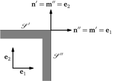
Figure 2: The coordinate edge $\mathcal{E}_{12}$.

it is constructed as a special case of the edge in Figure 1, by taking $\mathcal{S}_{1}$ and $\mathcal{S}_{2}$ for $\mathcal{S}^{\prime\prime}$ and $\mathcal{S}^{\prime}$, respectively, and by choosing $\mathbf{m}^{\prime}=\mathbf{e}_{2}$, $\mathbf{m}^{\prime\prime}=\mathbf{e}_{1}$ (such prescriptions are needed to identify $\mathcal{E}_{12}$ unequivocally); the coordinate edges $\mathcal{E}_{23}$ and $\mathcal{E}_{13}$ are similarly defined (Figure 3).

Figure 3: The coordinate edges $\mathcal{E}_{12}$, $\mathcal{E}_{23}$, $\mathcal{E}_{13}$.

With the use of (36) and (39) we define, respectively, the diffuse hypertractions $\mathbf{h}_{i}$ on the coordinate planes $\mathcal{S}_{i}$ and the concentrated forces $\mathbf{f}\,^{\mathrm{e}}_{ik}$ on the coordinate edges $\mathcal{E}_{ik}$, namely,

$$\mathbf{h}_{1}=\mathsf{H}[\mathbf{e}_{1}\otimes\mathbf{e}_{1}],$$ (50)

$$\mathbf{h}_{2}=\mathsf{H}[\mathbf{e}_{2}\otimes\mathbf{e}_{2}],$$

$$\mathbf{h}_{3}=\mathsf{H}[\mathbf{e}_{3}\otimes\mathbf{e}_{3}],$$

and

$$\mathbf{f}\,^{\mathrm{e}}_{12} =\mathsf{H}[\mathbf{e}_{1}\otimes\mathbf{e}_{2}+\mathbf{e}_{2}\otimes\mathbf{e}_{1}]=2\,\mathsf{H}[\mathbf{e}_{1}\otimes\mathbf{e}_{2}],$$ (51)

$$\mathbf{f}\,^{\mathrm{e}}_{13} =\mathsf{H}[\mathbf{e}_{1}\otimes\mathbf{e}_{3}+\mathbf{e}_{3}\otimes\mathbf{e}_{1}]=2\,\mathsf{H}[\mathbf{e}_{1}\otimes\mathbf{e}_{3}],$$

$$\mathbf{f}\,^{\mathrm{e}}_{23} =\mathsf{H}[\mathbf{e}_{2}\otimes\mathbf{e}_{3}+\mathbf{e}_{3}\otimes\mathbf{e}_{2}]=2\,\mathsf{H}[\mathbf{e}_{2}\otimes\mathbf{e}_{3}],$$

where we have accounted for the required symmetry of $\mathsf{H}$, expressed by (16). We now show that the six vectors $\mathbf{h}_{i}$ and $\mathbf{f}\,^{\mathrm{e}}_{ik}$ (each of which does depend on the Cartesian basis chosen) allow for the construction of a basis-independent representation formula for the hyperstress tensor $\mathsf{H}$.

Indeed, we know that

$$\mathsf{H}=\sum_{ijk}H_{ijk}\mathbf{e}_{i}\otimes\mathbf{e}_{j}\otimes\mathbf{e}_{k};$$ (52)

again taking the index symmetry of $H_{ijk}$ into account, this sum can be rewritten as

$$\mathsf{H} =\sum_{j}\sum_{i}H_{ijj}\mathbf{e}_{i}\otimes\mathbf{e}_{j}\otimes\mathbf{e}_{j}+\sum_{j\neq k}\sum_{i}H_{ijk}\mathbf{e}_{i}\otimes\mathbf{e}_{j}\otimes\mathbf{e}_{k}$$ (53)

$$=\sum_{j}\sum_{i}H_{ijj}\mathbf{e}_{i}\otimes\mathbf{e}_{j}\otimes\mathbf{e}_{j}+\sum_{j<k}\sum_{i}H_{ijk}\mathbf{e}_{i}\otimes(\mathbf{e}_{j}\otimes\mathbf{e}_{k}+\mathbf{e}_{k}\otimes\mathbf{e}_{j}).$$

Since

$$H_{ijk}=\mathbf{e}_{i}\cdot\mathsf{H}[\mathbf{e}_{j}\otimes\mathbf{e}_{k}]$$ (54)

we deduce that

$$H_{ijk}=\frac{1}{2}\mathbf{e}_{i}\cdot\mathsf{H}[\mathbf{e}_{j}\otimes\mathbf{e}_{k}+\mathbf{e}_{k}\otimes\mathbf{e}_{j}].$$ (55)

Thus, in view of (50),

$$H_{ijj}=\frac{1}{2}\mathbf{e}_{i}\cdot\mathsf{H}[\mathbf{e}_{j}\otimes\mathbf{e}_{j}+\mathbf{e}_{j}\otimes\mathbf{e}_{j}]=\frac{1}{2}\mathbf{e}_{i}\cdot 2\mathbf{h}_{j}=\mathbf{e}_{i}\cdot\mathbf{h}_{j},$$ (56)

which implies that

$$\mathbf{h}_{j}=\hat{}\mathbf{h}(x,\mathbf{e}_{j})=\sum_{i}\widehat{H}_{ijj}(x)\mathbf{e}_{i}\quad(\mbox{no sum over $j$}).$$ (57)

Similarly, for $j<k$,

$$H_{ijk}=\frac{1}{2}\mathbf{e}_{i}\cdot\mathsf{H}[\mathbf{e}_{j}\otimes\mathbf{e}_{k}+\mathbf{e}_{k}\otimes\mathbf{e}_{j}]=\frac{1}{2}\mathbf{e}_{i}\cdot\mathbf{f}\,^{\mathrm{e}}_{jk},$$ (58)

which implies that

$$\mathbf{f}\,^{\mathrm{e}}_{jk}=\hat{}\mathbf{f}\,^{\mathrm{e}}(x,{\mathcal{E}}_{jk})=2\sum_{i}\widehat{H}_{ijk}(x)\mathbf{e}_{i},\quad(\mbox{for $j<k$}).$$ (59)

By substitution of (57) and (59) in (53), we deduce the desired representation formula for $\widehat{\mathsf{H}}$ in terms of $\hat{}\mathbf{h}$ and $\hat{}\mathbf{f}\,^{\mathrm{e}}$:

$$\widehat{\mathsf{H}}(x)=\sum_{j}\hat{}\mathbf{h}(x,\mathbf{e}_{j})\otimes\mathbf{e}_{j}\otimes\mathbf{e}_{j}+\frac{1}{2}\sum_{j<k}\hat{}\mathbf{f}\,^{\mathrm{e}}(x,{\mathcal{E}}_{jk})\otimes(\mathbf{e}_{j}\otimes\mathbf{e}_{k}+\mathbf{e}_{k}\otimes\mathbf{e}_{j}).$$ (60)

We regard this formula as the main result of this paper.

4 Second-gradient materials with no edge tractions

We now ask the following question: which restrictions on $\mathsf{H}$ can be deduced from the assumption that no forces act on any edge, real or imagined? Said differently: is the hyperstress necessarily everywhere null in a second-gradient material body deemed to be unable to develop edge tractions?

Let us then suppose that, at a fixed body point $x$, we have that $\hat{}\mathbf{f}\,^{\mathrm{e}}(x,\cdot)\equiv\bm{0}$, so that the forces on all coordinate edges are zero, whatever the basis. Under this assumption, we have from (60) that, with respect to any given basis, $\mathsf{H}$ can be writte as:

$$\mathsf{H}=\sum_{j}\mathbf{h}_{j}\otimes\mathbf{e}_{j}\otimes\mathbf{e}_{j}$$ (61)

(recall that vectors $\mathbf{h}_{j}$ do depend on the chosen basis). Now, consider a new orthonormal basis $\bar{\mathbf{e}}_{i}$, obtained from $\mathbf{e}_{i}$ by a rotation about $\mathbf{e}_{3}$ of some angle $\theta$:

$$\bar{\mathbf{e}}_{1}=\cos\theta\,{\mathbf{e}}_{1}+\sin\theta\,{\mathbf{e}}_{2},\quad\bar{\mathbf{e}}_{2}=-\sin\theta\,{\mathbf{e}}_{1}+\cos\theta\,{\mathbf{e}}_{2},\quad\bar{\mathbf{e}}_{3}={\mathbf{e}}_{3},$$ (62)

and compute

$${\bar{\mathbf{f}}}\,^{\mathrm{e}}_{12}=2\mathsf{H}[\bar{\mathbf{e}}_{1}\otimes\bar{\mathbf{e}}_{2}].$$

It turns out that

$${\bar{\mathbf{f}}}\,^{\mathrm{e}}_{12} =-2\sin\theta\cos\theta\,\underbrace{\mathsf{H}[{\mathbf{e}}_{1}\otimes{\mathbf{e}}_{1}]}_{=\,\mathbf{h}_{1}}+2\sin\theta\cos\theta\,\underbrace{\mathsf{H}[{\mathbf{e}}_{2}\otimes{\mathbf{e}}_{2}]}_{=\,\mathbf{h}_{2}}$$ (63)

$$\quad\quad+\cos^{2}\theta\,\underbrace{2\mathsf{H}[{\mathbf{e}}_{1}\otimes{\mathbf{e}}_{2}]}_{=\,{{\mathbf{f}}}\,^{\mathrm{e}}_{12}}-\sin^{2}\theta\,\underbrace{2\mathsf{H}[{\mathbf{e}}_{2}\otimes{\mathbf{e}}_{1}]}_{=\,{{\mathbf{f}}}\,^{\mathrm{e}}_{12}}\,.$$

But, because the edge tractions ${\bar{\mathbf{f}}}\,^{\mathrm{e}}_{12}$ and ${{\mathbf{f}}}\,^{\mathrm{e}}_{12}$ must be zero by assumption, it follows from the last relation that, for all $\theta$,

$$\bm{0}=2\sin\theta\cos\theta(\mathbf{h}_{2}-\mathbf{h}_{1});$$ (64)

this implies that $\mathbf{h}_{1}=\mathbf{h}_{2}$. Moreover, for a rotation about $\mathbf{e}_{1}$, the same argument yields that $\mathbf{h}_{2}=\mathbf{h}_{3}$. Then, we can set

$$\mathbf{h}:=\mathbf{h}_{1}=\mathbf{h}_{2}=\mathbf{h}_{3},$$ (65)

and write (61) as follows:

$$\mathsf{H}=\mathbf{h}\otimes\sum_{j}\mathbf{e}_{j}\otimes\mathbf{e}_{j}=\mathbf{h}\otimes\mathbf{I}.$$ (66)

We conclude that a constitutive lack of edge forces implies that

$$\mathsf{H}=\mathbf{h}\otimes\mathbf{I},$$ (67)

for some vector $\mathbf{h}$; such $\mathbf{h}$ does not depend on the basis chosen for the argument, because $3\mathbf{h}=\mathsf{H}[\mathbf{I}]$. Conversely, if $\mathsf{H}$ admits the representation (67) for some vector $\mathbf{h}$, then it readily follows from (39) and (22) that all edge tractions are zero. Indeed,

$$\hat{}\mathbf{f}\,^{\mathrm{e}}(\mathcal{E}) =\mathsf{H}[\mathbf{n}^{\prime}\otimes\mathbf{m}^{\prime}+\mathbf{n}^{\prime\prime}\otimes\mathbf{m}^{\prime\prime}]$$ (68)

$$=\big{(}\mathbf{I}\cdot(\mathbf{n}^{\prime}\otimes\mathbf{m}^{\prime}+\mathbf{n}^{\prime\prime}\otimes\mathbf{m}^{\prime\prime})\big{)}\,\mathbf{h}$$

$$=(\mathbf{n}^{\prime}\cdot\mathbf{m}^{\prime}+\mathbf{n}^{\prime\prime}\cdot\mathbf{m}^{\prime\prime})\,\mathbf{h}=\bm{0},$$

since $(\mathbf{n}^{\prime},\mathbf{m}^{\prime})$ and $(\mathbf{n}^{\prime\prime},\mathbf{m}^{\prime\prime})$ are pairs of orthogonal vectors.

Remark. An alternative proof of the assertion leading to (67) was given by Forte and Vianello in [3]. Here it is. If there are no edge tractions, then

$$\mathbf{w}\cdot\mathsf{H}[\mathbf{n}\otimes\mathbf{m}]=0$$ (69)

for any given vector $\mathbf{w}$ and for all pairs of orthonormal vectors $\mathbf{n}$, $\mathbf{m}$. Thus, the second-order symmetric tensor ${\mathsf{H}}^{T}\mathbf{w}$, whose components are $({\mathsf{H}}^{T}\mathbf{w})_{jk}=w_{i}H_{ijk})$, must have diagonal form with respect to any basis:

$$\mathbf{w}\mathsf{H}=\lambda(\mathbf{w})\mathbf{I},\quad\mbox{for some scalar-valued function $\lambda(\mathbf{w})$}.$$ (70)

However, since the left side of this relation is linear in $\mathbf{w}$, there must be a vector $\mathbf{h}$ such that $\lambda(\mathbf{w})=\mathbf{h}\cdot\mathbf{w}$. But,

$$\mathbf{w}\mathsf{H}=(\mathbf{h}\cdot\mathbf{w})\,\mathbf{I}\quad\Rightarrow\quad\mathsf{H}=\mathbf{h}\otimes\mathbf{I}\,.$$ (71)

Remark. No mathematically precise notion of fluidity and solidity has been suggested so far for complex continua. A current malpractice is to base the distinction on whether the first-gradient stress arising in response to deformation histories complies with the one or the other of the group-theoretic recipes proposed by Noll to sort simple fluids from simple solids. Recently, one of us [13] came up with a notion of macroscopic aggregation state of matter based on an invariance requirement of the internal power expenditure under classes of changes of the reference placement different for fluid and solid simple materials. This notion is formally easy to generalize to complex materials, although the analysis involved is far from trivial. We develop these issues in full in a forthcoming paper [14]. Suffice it to mention here a class of Navier-Stokes$-\alpha$ fluids, that is, of second-gradient materials obeying, among others to be introduced shortly, the following constitutive prescription for the power expenditure of hypertractions:

$$\mathsf{H}\cdot\operatorname{grad}\negthinspace^{2}\mathbf{v}=\mathbf{g}\cdot\operatorname{curl}\operatorname{curl}\mathbf{v}\,.$$ (72)

In view of the differential identity:

$$\operatorname{curl}\operatorname{curl}\mathbf{v}=\operatorname{grad}(\operatorname{div}\mathbf{v})-\Delta\mathbf{v},$$ (73)

it is not difficult to see that

$$\mathbf{g}\cdot\operatorname{curl}\operatorname{curl}\mathbf{v}=\mathsf{H}_{1}\cdot\operatorname{grad}\negthinspace^{2}\mathbf{v}+\mathsf{H}_{2}\cdot\operatorname{grad}\negthinspace^{2}\mathbf{v};$$ (74)

with

$$(\mathsf{H}_{1})_{ijk}=\frac{1}{2}\big{(}\delta_{ij}g_{k}+\delta_{ik}g_{j}\big{)}\quad\textrm{and}\quad\mathsf{H}_{2}=-\mathbf{g}\otimes\mathbf{I}.$$ (75)

Furthermore, if

$$\operatorname{div}\mathbf{v}=0,$$ (76)

as is customarily stipulated in microfluidics, then

$$\mathbf{g}\cdot\operatorname{curl}\operatorname{curl}\mathbf{v}=-\mathbf{g}\cdot\Delta\mathbf{v}.$$ (77)

Thus, (i) $\mathsf{H}_{1}$ can be interpreted as the reactive hyperstress associated to the second-gradient consequence of the standard incompressibility constraint; (ii) $\mathsf{H}_{2}$, the active hyperstress, induces no edge hypertractions; and, (iii) if one chooses the simplest constitutive prescription

$$\mathbf{g}=\zeta\,\Delta\mathbf{v},\quad\zeta>0,$$ (78)

then the regularizing term $-\zeta\,\Delta(\Delta\mathbf{v})$ typical of the Navier-Stokes$-\alpha$ flow equation [4] appears in the balance equation.

5 Appendix

We collect here some subsidiary material, with the purpose of improving the readability and self-containment of our paper.

5.1 Observer changes

By an observer change we mean the following transformation rule for position vectors of space points:

$$\mathbf{x}^{+}={\mathcal{O}}(\mathbf{x})=\mathbf{q}+\mathbf{Q}\mathbf{x},\quad\mathbf{x}:=x-o,$$ (79)

where $\mathbf{q}$ is an arbitrary time-dependent translation and $\mathbf{Q}$ an arbitrary time-dependent rotation about point $o$. The related transformation rule for velocities is:

$$\mathbf{v}^{+}=\dot{}\mathbf{q}+\mathbf{Q}\mathbf{v}+\mathbf{W}\mathbf{x}^{+},\quad\mathbf{W}:=\dot{}\mathbf{Q}\mathbf{Q}^{T}=-\mathbf{W}^{T},$$ (80)

where all of the parameters $\dot{}\mathbf{q}$, $\mathbf{Q}$, and $\mathbf{W}$, can take arbitrary values at any chosen time (cf. (2)). It follows from (79) that

$$\operatorname{grad}^{+}(\cdot)=\operatorname{grad}(\cdot)\mathbf{Q}^{T}\,.$$ (81)

Hence, as to the velocity gradient, one finds that

$$(\operatorname{grad}\mathbf{v})^{+}=\mathbf{Q}(\operatorname{grad}\mathbf{v})\mathbf{Q}^{T}+\mathbf{W}.$$ (82)

5.2 Rotational invariance of the internal power expenditure

The rotational invariance of the specific internal power expenditure is the requirement that, at all points of $B$,

$$\mathbf{T}\cdot\operatorname{grad}\mathbf{v}+\mathsf{H}\cdot\operatorname{grad}\negthinspace^{2}\mathbf{v}=\mathbf{T}^{+}\cdot(\operatorname{grad}\mathbf{v})^{+}+\mathsf{H}^{+}\cdot(\operatorname{grad}\negthinspace^{2}\mathbf{v})^{+},$$ (83)

where

$$\mathbf{T}^{+}={\mathcal{O}}(\mathbf{T}),\quad\mathsf{H}^{+}={\mathcal{O}}(\mathsf{H}),\quad\textrm{etc.}$$ (84)

In order to discuss the consequences of this requirement, it is convenient to define the action of the rotation group on second- and third-order tensors: in cartesian components,

$$[\mathbf{Q}\ast\mathbf{A}]_{ij}:=Q_{ip}Q_{jq}A_{pq},\qquad[\mathbf{Q}\ast\mathsf{H}]_{ijk}:=Q_{ip}Q_{jq}Q_{kr}H_{pqr};$$ (85)

in absolute notation,

$$\mathbf{Q}\ast\mathbf{A}=\mathbf{Q}\mathbf{A}\mathbf{Q}^{T},\qquad(\mathbf{Q}\ast\mathsf{H})[\mathbf{a}\otimes\mathbf{b}]\cdot\mathbf{c}=\mathsf{H}[\mathbf{Q}^{T}\mathbf{a}\otimes\mathbf{Q}^{T}\mathbf{b}]\cdot\mathbf{Q}^{T}\mathbf{c}\,.$$ (86)

Notice that, for any pair of rotations $\mathbf{Q}_{1}$ and $\mathbf{Q}_{2}$,

$$(\mathbf{Q}_{1}\mathbf{Q}_{2})\ast\mathbf{A}=\mathbf{Q}_{1}\ast(\mathbf{Q}_{2}\ast\mathbf{A}),\qquad(\mathbf{Q}_{1}\mathbf{Q}_{2})\ast\mathsf{H}=\mathbf{Q}_{1}\ast(\mathbf{Q}_{2}\ast\mathsf{H});$$ (87)

moreover,

$$(\mathbf{Q}\ast\mathbf{A})\cdot\mathbf{B}=\mathbf{A}\cdot(\mathbf{Q}^{T}\ast\mathbf{B}),\qquad(\mathbf{Q}\ast\mathsf{H})\cdot\mathsf{K}=\mathsf{H}\cdot(\mathbf{Q}^{T}\ast\mathsf{K}),$$ (88)

for all pairs of second- and third-order tensors $\mathbf{A}$, $\mathbf{B}$, $\mathsf{H}$, $\mathsf{K}$ and for all rotations $\mathbf{Q}$.

With this notation, the transformation rule (82) becomes:

$$(\operatorname{grad}\mathbf{v})^{+}=\mathbf{Q}\ast(\operatorname{grad}\mathbf{v})+\mathbf{W}.$$ (89)

Moreover, by an application of (81), we readily deduce the transformation rule for the second gradient of velocity:

$$(\operatorname{grad}\negthinspace^{2}\mathbf{v})^{+}=\mathbf{Q}\ast(\operatorname{grad}\negthinspace^{2}\mathbf{v}).$$ (90)

Thus, (83) can be rewritten as:

$$\mathbf{T}\cdot\operatorname{grad}\mathbf{v}+\mathsf{H}\cdot\operatorname{grad}\negthinspace^{2}\mathbf{v}=\mathbf{T}^{+}\cdot(\mathbf{Q}\ast\operatorname{grad}\mathbf{v}+\mathbf{W})+\mathsf{H}^{+}\cdot(\mathbf{Q}\ast\operatorname{grad}\negthinspace^{2}\mathbf{v}),$$ (91)

or rather, equivalently in view of (88),

$$\mathbf{T}\cdot\operatorname{grad}\mathbf{v}+\mathsf{H}\cdot\operatorname{grad}\negthinspace^{2}\mathbf{v}=(\mathbf{Q}^{T}\ast\mathbf{T}^{+})\cdot\operatorname{grad}\mathbf{v}+\mathbf{T}^{+}\cdot\mathbf{W}+(\mathbf{Q}^{T}\ast\mathsf{H}^{+})\cdot\operatorname{grad}\negthinspace^{2}\mathbf{v}.$$ (92)

Since all of the multipliers $\operatorname{grad}\mathbf{v}$, $\operatorname{grad}\negthinspace^{2}\mathbf{v}$ and $\mathbf{W}$ can be prescribed arbitrarily and independently from each other, we conclude that $\mathbf{T}$ must be symmetric and, moreover, that the following transformation rules must hold:

$$\mathbf{T}^{+}=\mathbf{Q}\ast\mathbf{T},\qquad\mathsf{H}^{+}=\mathbf{Q}\ast\mathsf{H}$$ (93)

(cf. (27)). This conclusion fully generalizes the well known result for simple (first order) materials.

References

• [1] Dell’Isola, F., Seppecher, P.: Edge contact forces and quasi-balanced power. Meccanica 32, 33–52 (1997)
• [2] Dunn, J.E., Serrin, J.: On the thermodynamics of interstitial working. Arch. Rational Mech. Anal. 88, 95–133 (1985)
• [3] Forte, S., Vianello, M.: On surfaces stresses and edge forces. Rend. Mat. Appl. 8(3), 409–426 (1988)
• [4] Fried, E., Gurtin, M.E.: Tractions, balances, and boundary conditions for nonsimple materials with application to liquid flow at small-length scales. Arch. Rational Mech. Anal. 182(3), 513–554 (2006). DOI 10.1007/s00205-006-0015-7
• [5] Germain, P.: Sur l’application de la méthode des puissances virtuelles en mécanique des milieux continus. C. R. Acad. Sc. Paris Série A 274, 1051–1055 (1972)
• [6] Germain, P.: La méthode des puissances virtuelles en mécanique des milieux continus. première partie: Théorie du second gradient. J. Mécanique 12, 235–274 (1973)
• [7] Germain, P.: The method of virtual power in continuum mechanics. part 2: Microstructure. SIAM J. Appl. Math. 25, 556–575 (1973)
• [8] Gurtin, M.E., Murdoch, I.: A continuum theory of elastic material surfaces. Arch. Rational Mech. Anal. 57, 291–323 (1974)
• [9] Korteweg, D.J.: Sur la forme que prennent les equations du mouvement des fluides si l’on tient compte des forces capillaires. Arch. Neerl. Sci. Ex. Nat. 6, 1–24 (1901)
• [10] Maugin, G.A.: The method of virtual power in continuum mechanics: applications to coupled fields. Acta Mech. 35, 1–70 (1980)
• [11] Noll, W., Virga, E.G.: On edge interactions and surface tension. Arch. Rational Mech. Anal. 111(1), 1–31 (1990)
• [12] Podio-Guidugli, P.: Contact interactions, stress, and material symmetry, for nonsimple elastic materials. Theoretical and Applied Mechanics 28-29, 261–276 (2002)
• [13] Podio-Guidugli, P.: On the aggregation state of simple materials. In: Šilhavý (ed.) Mathematical modeling of bodies with complicated bulk and boundary behavior, Quaderni di Matematica, vol. 20, pp. 159–168 (2007)
• [14] Podio-Guidugli, P., Vianello, M.: Fluidity and solidity notions for complex materials. (2009). Unpublished.
• [15] Toupin, R.A.: Elastic materials with couple stresses. Arch. Rational Mech. Anal. 11, 385–414 (1962)
• [16] Toupin, R.A.: Theories of elasticity with couple-stresses. Arch. Rational Mech. Anal. 17, 85–112 (1964)