Understanding mixing efficiency in the oceans:
Do the nonlinearities of the equation of state for seawater matter?

Zusammenfassung

There exist two central measures of turbulent mixing in turbulent stratified fluids that are both caused by molecular diffusion: 1) the dissipation rate $D(APE)$ of available potential energy $APE$; 2) the turbulent rate of change $W_{r,turbulent}$ of background gravitational potential energy $GPE_{r}$. So far, these two quantities have often been regarded as the same energy conversion, namely the irreversible conversion of $APE$ into $GPE_{r}$, owing to the well known exact equality $D(APE)=W_{r,turbulent}$ for a Boussinesq fluid with a linear equation of state. Recently, however, Tailleux (2009) pointed out that the above equality no longer holds for a thermally-stratified compressible, with the ratio $\xi=W_{r,turbulent}/D(APE)$ being generally lower than unity and sometimes even negative for water or seawater, and argued that $D(APE)$ and $W_{r,turbulent}$ actually represent two distinct types of energy conversion, respectively the dissipation of $APE$ into one particular subcomponent of internal energy called the ‘dead’ internal energy $IE_{0}$, and the conversion between $GPE_{r}$ and a different subcomponent of internal energy called ’exergy’ $IE_{exergy}$. In this paper, the behaviour of the ratio $\xi$ is examined for different stratifications having all the same buoyancy frequency $N$ vertical profile, but different vertical profiles of the parameter $\Upsilon=\alpha P/(\rho C_{p})$, where $\alpha$ is the thermal expansion coefficient, $P$ the hydrostatic pressure, $\rho$ the density, and $C_{p}$ the specific heat capacity at constant pressure, the equation of state being that for seawater for different particular constant values of salinity. It is found that $\xi$ and $W_{r,turbulent}$ depend critically on the sign and magnitude of $d\Upsilon/dz$, in contrast with $D(APE)$, which appears largely unaffected by the latter. These results have important consequences for how the mixing efficiency should be defined and measured in practice, which are discussed.

As is well known, turbulent diffusive mixing is a physical process that it is crucially important to parameterise well in numerical ocean models in order to achieve realistic simulations of the water mass properties and of the so-called meridional overturning circulation (Gregg, 1987), which are two essential components of the large-scale ocean circulation that may interact with Earth climate. For this reason, much effort has been devoted over the past decades toward understanding the physics of turbulent mixing in stratified fluids, one important goal being the design of physically-based parameterisations of irreversible mixing processes for use in numerical ocean climate models.

At a fundamental level, turbulent molecular diffusion in stratified fluids is important for at least two distinct — although inter-related — reasons: 1) for transporting heat diffusively across isopycnal surfaces – a process often referred to as ‘diapycnal mixing’; 2) for dissipating available potential energy, which contributes for a significant fraction — often called the mixing efficiency — of the total dissipation of available mechanical energy $ME$, i.e., the sum of total kinetic energy $KE$ and available potential energy $APE$, which are defined by:

$$KE=\int_{V}\rho\frac{{\bf v}^{2}}{2}dV,$$ (1)

$$APE=\underbrace{\int_{V}\rho\left(gz+I\right)dV}_{PE}-\underbrace{\int_{V}\rho\left(gz_{r}+I_{r}\right)dV}_{PE_{r}},$$ (2)

where $\rho$ is the density, ${\bf v}=(u,v,w)$ is the three-dimensional velocity vector, $g$ is the acceleration of gravity, $z$ is the vertical coordinate increasing upward, and $I$ the specific internal energy. The APE is defined as in Lorenz (1955) as the difference between the potential energy $PE$ of the fluid (i.e., the sum of the gravitational potential energy $GPE$ plus internal energy $IE$) minus the potential energy $PE_{r}$ of a reference state that is the state of minimum potential energy achievable in an adiabatic re-arrangement of the fluid parcels. As shown by Winters & al. (1995), the $APE$ and $PE_{r}$ play a fundamental in the modern theory of turbulent mixing owing to the fact that by construction $PE_{r}$ is only affected by irreversible processes; as a result, measuring the time evolution of the reference state provides a direct and objective way to quantify the amount of irreversible mixing taking place during turbulent mixing events, which is now commonly exploited to diagnose mixing in numerical experiments, e.g., Peltier & Caulfield (2003).

In the oceans, turbulent diapycnal mixing is required to transfer heat downward from the surface at a sufficiently rapid rate to balance the cooling of the deep ocean by high-latitudes deep water formation. In the oceanographic literature, the most widely used approach to parameterise the vertical (diapycnal) eddy diffusivity $K_{\rho}$ is based on the Osborn-Cox model (Osborn and Cox (1972)):

$$K_{\rho}=\frac{\varepsilon_{P}}{N^{2}}=\frac{\gamma_{mixing}\,\,\varepsilon_{K}}{N^{2}},$$ (3)

which expresses $K_{\rho}$ in terms of either the turbulent viscous kinetic energy dissipation $\varepsilon_{K}$ or turbulent diffusive dissipation of available potential energy $\varepsilon_{P}$, where $N^{2}$ is the squared buoyancy frequency, and $\gamma_{mixing}=\varepsilon_{P}/\varepsilon_{K}$ is the ratio of the APE to KE dissipation, which is often called the ‘mixing efficiency’, e.g. Lindborg & Brethouwer (2008). Expressing $K_{\rho}$ in terms of $\varepsilon_{K}$ appears to have been first proposed by Lilly & al. (1974) and Weinstock (1978) in the context of stratospheric turbulent mixing, and adapted to the oceanographic case by Osborn (1980). The definition of mixing efficiency as a dissipations ratio adopted in this paper appears to have been first proposed by Oakey (1982).

Since both $\epsilon_{P}$ and $\varepsilon_{K}$ are linked to the dissipation of mechanical energy of which $KE$ and $APE$ represent the two main dynamically important forms, Eq. (3) makes it clear that turbulent diapycnal mixing is directly related to the mechanical energy input in the oceans, but this link has been so far very rarely exploited in numerical ocean models. Rather, $K_{\rho}$ is often regarded as a tunable parameter whose value is adjusted to reproduce the main observed features of the oceanic stratification. Such an approach was used by Munk (1966), who assumed the stratification to obey the vertical advective/diffusive balance:

$$w\frac{\partial\theta}{\partial z}=\frac{\partial}{\partial z}\left(K_{\rho}\frac{\partial\theta}{\partial z}\right),$$ (4)

where $\theta$ is the potential temperature, and $w$ the vertical velocity. Physically, Eq. (4) states that the upward advection of cold water is balanced by the downward turbulent diffusion of heat, the rate of upwelling being set up by the rate of deep water formation. By using Eq. (4) as a model for stratification profiles in the Pacific, Munk (1966) concluded that the canonical value $K_{\rho}=10^{-4}\,{\rm m^{2}/s}$ was apparently needed to explain the observed structure of the oceanic thermocline. Subsequently, however, the validity of Munk (1966)’s approach was questioned, as several observational studies found $K_{\rho}$ in the ocean interior to be typically smaller by an order of magnitude than Munk’s value, e.g., see Ledwell & al (1998) and the review by Gregg (1987). However, it seems widely recognised today that $K_{\rho}$ is highly variable spatially, prompting Munk & Wunsch (1998) to re-interpret the value $K_{\rho}=10^{-4}\,{\rm m^{2}.s^{-1}}$ as resulting from the overall effect of weak interior values combined with intense turbulent mixing in coastal areas or over rough topography.

While the above approach is useful, it does not exploit the link between $K_{\rho}$ and the mechanical sources of stirring suggested by Eq. (3). Clarifying this link was pioneered by Munk & Wunsch (1998), who translated the advection/diffusion balance into one for the gravitational potential energy budget, which they argue must be a balance between the rate of $GPE$ loss due to cooling and the rate of $GPE$ increase due to turbulent diffusive mixing, i.e.,

$$\left|\frac{d(GPE_{r})}{dt}\right|_{cooling}\approx\left|\frac{d(GPE_{r})}{dt}\right|_{mixing},$$ (5)

this result being obtained by multiplying Eq. (4) by $\alpha_{\theta}\rho_{0}gz$, after some manipulation involving integration by parts and the neglect of surface heating, where $\alpha_{\theta}$ is the thermal expansion, $g$ the acceleration of gravity, $\rho_{0}$ a reference density, and $z$ the vertical coordinate pointing upward. The subscript $r$ is added here because it can be shown that Munk & Wunsch (1998) must actually pertain to the background $GPE_{r}$ budget, rather than the $AGPE$ budget, as shown by Tailleux (2009). This follows from the fact that cooling and turbulent molecular diffusion act as a $GPE$ sink and source only for the background $GPE_{r}$, as it is the opposite that holds for $AGPE$. If one assumes that density is primarily controlled by temperature for simplicity, the effect of mixing on $GPE_{r}$ is thus given by:

$$\left|\frac{d(GPE_{r})}{dt}\right|_{mixing}=-\int_{V}\rho_{0}\alpha_{\theta}gz\frac{\partial}{\partial z}\left(K_{\rho}\frac{\partial\theta}{\partial z}\right)dV$$

$$=\int_{V}\rho_{0}K_{\rho}N^{2}\left(1+\frac{z}{\alpha_{\theta}}\frac{\partial\alpha_{\theta}}{\partial z}\right)dV,$$ (6)

by using the result that $N^{2}=\alpha_{\theta}g\partial\theta/\partial z$ in absence of salinity effects, and by assuming $z=0$ at the ocean surface, and no flux through the ocean bottom. In their paper, Munk & Wunsch (1998) neglected the nonlinearities of the equation of state, which amounts to regard $\alpha_{\theta}$ as constant, in which case the above expression becomes:

$$\left|\frac{d(GPE_{r})}{dt}\right|_{mixing}\approx\int_{V}\rho_{0}K_{\rho}N^{2}dV.$$ (7)

By using Eq. (3), assuming $\gamma_{mixing}$ constant, this formula can be rewritten as follows:

$$\left|\frac{d(GPE_{r})}{dt}\right|_{mixing}=\underbrace{\int_{V}\rho_{0}\varepsilon_{P}dV}_{D(APE)}=\gamma_{mixing}\underbrace{\int_{V}\rho_{0}\varepsilon_{K}dV}_{D(KE)}$$ (8)

where $D(APE)$ and $D(KE)$ are the total volume-integrated diffusive dissipation of available potential energy and viscous dissipation of kinetic energy respectively. To conclude, Munk & Wunsch (1998) linked the dissipation to production terms by assuming the balance $D(KE)=G(KE)$, where $G(KE)$ is the work rate done by the mechanical forcing due to the winds and tides. As a result, the above formula yields:

$$G(KE)=\frac{1}{\gamma_{mixing}}\left|\frac{d(GPE)}{dt}\right|_{cooling}.$$ (9)

By estimating the rate of $GPE$ loss due to cooling to be $0.4\,{\rm TW}$, and by using the canonical value $\gamma_{mixing}=0.2$, Munk & Wunsch (1998) concluded that $G(KE)=O(2\,{\rm TW})$ of mechanical energy input was required to sustain turbulent diapycnal mixing in the oceans. Since the work of the wind stress against the surface geostrophic velocity is widely agreed to be $O(1\,{\rm TW})$, Munk & Wunsch (1998) suggested that the shortfall should be explained by the work rate done by the tides. The issue remains controversial, however, because the role of the surface buoyancy forcing is not sufficiently well understood, as discussed in Tailleux (2009).

Another important issue in assessing the uncertainties associated with Eq. (9) concerns the importance of the nonlinearities of the equation of state, neglected by Munk & Wunsch (1998). As is well known, the nonlinearities of the equation of state are mostly responsible for the fluid “contracting upon mixing”. This contraction is responsible for the actual increase in $GPE_{r}$ due to mixing to be less than for a linear equation of state. In Eq. (6), this can be seen from the fact that $\partial\alpha_{\theta}/\partial z$ is usually positive for a stably stratified fluid. Since $z$ is negative by assumption, it follows that a correction factor is required that modifies Eq. (8) as follows:

$$\left|\frac{d(GPE)}{dt}\right|_{mixing}=(1-C_{m})D(APE)$$

$$=(1-C_{m})\gamma_{mixing}D(KE).$$ (10)

where $C_{m}>0$, which in turn modifies Munk & Wunsch (1998)’s constraint (Eq. (9)) as follows:

$$G(KE)=\frac{1}{\xi\gamma_{mixing}}\left|\frac{d(GPE)}{dt}\right|_{cooling}$$ (11)

where $\xi=1-C_{m}<1$. Based on the above arguments, Munk & Wunsch (1998)’s results are expected to underestimate the constraint on $G(KE)$, to the extent that $\gamma_{mixing}$ and the rate of $GPE_{r}$ loss due to cooling can be kept fixed. This point was first pointed out by Gnanadesikan & al. (2005) who emphasised the importance of cabelling. Discussing the value of $C_{m}$ or $\xi$ to be used in Eq. (9) is beyond the scope of this paper. Note, however, that it is possible to construct stratifications with $\xi$ not only smaller than one but also possibly even negative, as discussed by Fofonoff (1998, 2001). The latter cases are interesting, because they are such that $GPE_{r}$ decreases upon mixing, not increases, in contrast to what is usually assumed.

The main reason that $GPE_{r}$ is often assumed to increase as a result of turbulent mixing stems from that for an incompressible fluid with a linear equation of state, Eq. (8) states that:

$$\left|\frac{d(GPE)}{dt}\right|_{mixing}=D(APE),$$ (12)

i.e., that $GPE_{r}$ increases at the same rate that $APE$ decreases, which is classically interpreted as implying that the diffusively dissipated $APE$ must be irreversibly converted into $GPE_{r}$, e.g., Winters & al. (1995). Tailleux (2009) pointed out, however, that Eq. (12) is at best only a good approximation, not a true equality, since in reality the rates of $GPE_{r}$ increase and $APE$ decrease are never exactly equal, and sometimes even widely different, because of the nonlinear character of the equation of state.

In order to better understand how the net change in $GPE_{r}$ correlates with the total amount of $APE$ diffusively dissipated during an irreversible turbulent mixing event, it is useful to examine the process of turbulent mixing in the light of classical thermodynamic transformations. To make progress, the conditions under which the diffusive exchange of heat between fluid parcels takes place need to be known, but in practice this is problematic, for it would require solving the full compressible non-hydrostatic Navier-Stokes equations down to the diffusive scales. Fortunately, it is often the case that stratified fluids at low Mach numbers are close to hydrostatic equilibrium, suggesting that the diffusive heat exchange between parcels may reasonably be assumed to occur at approximately constant pressure. If so, irreversible diffusive mixing must then be close to be a process conserving the total potential energy $PE=APE+PE_{r}$ of the system, which implies that any amount $\Delta APE_{diff}<0$ of diffusively dissipated $APE$ must be irreversibly converted into background $PE_{r}$, viz.,

$$\Delta PE_{r}=-\Delta APE_{diff}>0.$$ (13)

The implications for the net change in $GPE_{r}$ can be determined from the definitions $PE_{r}=GPE_{r}+IE_{r}$, $APE=AGPE+AIE$, and $IE=AIE+IE_{r}$, which imply:

$$\Delta GPE_{r}=-\Delta APE_{diff}-\Delta IE_{r}$$ (14)

where $\Delta IE_{r}$ is the net change in background internal energy taking place during the irreversible mixing event. As a result, the quantities $\xi$ and $C_{m}$ previously defined become:

$$\xi=\frac{\Delta GPE_{r}}{|\Delta APE_{diff}|}=1-\frac{\Delta IE_{r}}{|\Delta APE_{diff}|},$$ (15)

$$C_{m}=\frac{\Delta IE_{r}}{|\Delta APE_{diff}|}.$$ (16)

Eqs. (15) and (16) are important, because they establish that the nonlinearities of the equation of state — which are responsible for the temperature and pressure dependence of $\alpha$ — can give rise to internal energy changes $\Delta IE_{r}$ comparable in magnitude with $\Delta APE_{diff}$ and $\Delta GPE_{r}$ during a turbulent mixing event. Such large $IE_{r}$ changes must in turn be associated with potentially large compressibility effects whose work against the pressure field may also expected to be large, as first demonstrated by Tailleux (2009). In other words, the above formula suggest that the nonlinearities of the equation of state may give rise to significant non-Boussinesq effects. So far, however, most numerical ocean models still make the incompressible and Boussinesq approximations, while at the same time using some version of the nonlinear equation of state for seawater. Such an approach yields values of $\xi$ and $C_{m}$ that are predicted by Eq. (6), but since those values ultimately derive from initially making the Boussinesq approximation, it is unclear whether they can take into account the nonlinear character of the equation of state in a fully consistent manner.

In fact, even when the net change $\Delta IE_{r}$ appears to be small or negligible, seemingly justifying the incompressible assumption, Tailleux (2009) argues that compressible effects may still be large, because one may show that $\Delta IE_{r}$ can be decomposed as follows:

$$\Delta IE_{r}=\Delta IE_{exergy}+\Delta IE_{0},$$ (17)

where $IE_{0}$ and $IE_{exergy}=IE_{r}-IE_{0}$ are two subcomponents of $IE_{r}$ called the ‘dead’ and ‘exergy’ components. Physically, $IE_{0}$ represents the internal energy of a notional thermodynamic equilibrium state of uniform temperature $T_{0}$, whereas $IE_{exergy}$ represents the internal energy associated with the vertical stratification of the reference state. An important result of Tailleux (2009) is that the net changes in $IE_{exergy}$ and $IE_{0}$ are related at leading order to $\Delta GPE_{r}$ and $\Delta APE_{diff}$ as follows:

$$\Delta GPE_{r}\approx-\Delta IE_{exergy},$$ (18)

$$\Delta IE_{0}\approx-\Delta APE_{diff}>0,$$ (19)

to a very good approximation in a nearly incompressible fluid such as water or seawater. These relations state that turbulent molecular diffusion primarily dissipates $APE$ into ‘dead’ internal energy $IE_{0}$, while simultaneously causing a transfer between $GPE_{r}$ and $IE_{exergy}$. Physically, the former effect results in an increase of the equivalent thermodynamic temperature $T_{0}$, whereas the latter effect results in the smoothing out of $dT_{r}/dz$. This contrasts with the standard interpretation that turbulent molecular diffusion irreversibly converts $APE$ into $GPE_{r}$, as proposed by Winters & al. (1995). The differences between the two interpretations are schematically illustrated in Fig. 1. The main reason why compressibility effects may be important even if $\Delta IE_{r}\approx 0$ is because volume changes are primarily determined by $\Delta IE_{exergy}$, not by $\Delta IE_{0}$ or $\Delta IE_{r}$.

As regards to the empirical determination of the mixing efficiency $\gamma_{mixing}=\varepsilon_{P}/\varepsilon_{K}$, the above remarks are important because $\Delta GPE_{r}$ and $|\Delta APE_{diff}|$ are currently widely thought to physically represent the same quantity, prompting many studies to actually estimate $\varepsilon_{P}$ from measuring the net changes in $GPE_{r}$, e.g., McEwan (1983a, b); Barry (2001). For the reasons discussed above, however, this makes sense only if $\xi$ can be ascertained to be close to unity, as if not, the relevant value of $\xi$ is then required. One of the main objective of this paper is to establish that the behaviour of $\xi$ is closely connected to the sign and amplitude of the following parameter:

$$\frac{d}{dz}\left(\frac{\alpha P}{\rho C_{p}}\right)$$ (20)

where $\alpha$ is the thermal expansion coefficient, $P$ is the pressure, $\rho$ is the density, and $C_{p}$ is the specific heat capacity at constant pressure, while salinity is assumed to be uniform throughout the domain. Physically, the parameter $\Upsilon=\alpha P/(\rho C_{p})=P\Gamma/T$, where $\Gamma$ is the adiabatic lapse rate, represents the fraction of the amount of heat $\delta Q$ received by a parcel in an isobaric process that can be converted into work. As a result, $\Upsilon$ is expected to be the main parameter controlling the net change in $GPE_{r}$ due to the turbulent diffusive heat exchange between fluid parcels.

From the viewpoint of turbulent mixing, the main difficulty posed by a nonlinear equation of state is to make it possible for different vertical stratification to share the same profile $N(z)$ without necessarily having the same $\Upsilon(z)$ vertical profile. From a dynamical viewpoint, this is not expected to be a problem as long as the dynamical evolution of $KE$ and $APE$, as well as $D(KE)$ and $D(APE)$, remain mostly controlled by $N(z)$ at leading order, as is usually assumed. If so, the dissipations ratio $D(APE)/D(KE)$, and hence the bulk mixing efficiency $\gamma_{mixing}$, can then be assumed to be unaffected by the nonlinearities of the equation of state at leading order. The main objective of this paper is to verify that $D(APE)$ appears indeed to be largely insensitive to the $\Upsilon(z)$ vertical profile, and hence mostly controlled by $N(z)$. If so, we can safely conclude that it must also be the case for $D(KE)$, since there is even less reasons to believe that the latter could be affected by $\Upsilon(z)$. This could be directly verified through direct numerical simulations of turbulent stratified mixing using a fully compressible Navier-Stokes equations solver, which we hope to report on in the future. On the other hand, the net change in $GPE_{r}$ is expected to be extremely sensitive to $\Upsilon(z)$. Most of the paper is devoted to verify that this is indeed the case, and to find ways to relate the net change in $GPE_{r}$ to the sign and magnitude of $d\Upsilon/dz$. Section 2 provides a theoretical formulation of the issue discussed. Section 3 discusses the methodology, while the results are presented in Section 4. Finally, section 5 summarises and discusses the results.

1 Theoretical formulation of the problem

1.1 Energetics of mixing

A key issue in the study of turbulent mixing is understanding the links between stirring and mixing. As first discussed by Eckart (1948), the two processes can be rigourously separated if one notes that the probability density functions (pdf in short) of the adiabatically conserved quantities (i.e., entropy and salt for seawater) are only affected by the irreversible mixing due to the molecular diffusion of heat and salt, but not by the adiabatic shuffling of the parcels due to the stirring process. The link with Lorenz (1955)’s available potential energy framework comes from the fact that Lorenz’s reference state, i.e., the state whose potential energy is minimised by an adiabatic re-arrangement of the fluid parcels, coincides with the above-mentioned pdf, which was exploited by Winters & al. (1995) to provide a new way to rigourously quantify irreversible mixing simply from diagnosing the temporal evolution of the reference state. In a Boussinesq fluid with a linear equation of state, the role of entropy is played by either temperature or density. In the following, the fluid will be assumed to be either freshwater or seawater with uniform salinity throughout the fluid.

As shown by Winters & al. (1995) (using somewhat different notations), the energetics of freely decaying turbulence in an insulated domain is based on the following evolution equations for the volume-integrated kinetic energy $(KE)$, available potential energy $(APE)$, and background gravitational potential energy $(GPE_{r})$:

$$\frac{d(KE)}{dt}=-C(KE,APE)-D(KE),$$ (21)

$$\frac{d(APE)}{dt}=C(KE,APE)-D(APE),$$ (22)

$$\frac{d(GPE_{r})}{dt}=W_{r,mixing}=W_{r,laminar}+W_{r,turbulent},$$ (23)

where $C(KE,APE)$ is the so-called buoyancy flux, which physically represents the reversible conversion between $KE$ and $APE$, while all other terms represent irreversible processes, with $D(KE)$ denoting the viscous dissipation of $KE$, $D(APE)$ the diffusive dissipation of $APE$, and $W_{r,mixing}$ the rate of change of $GPE_{r}$ due to molecular diffusion, which is customarily decomposed into a turbulent and laminar contribution. Note that the above equations are domain-averaged, not local formulations, which are expected to be well suited for understanding laboratory experiments of turbulent mixing for which lateral fluxes of $APE$ and $KE$ can be ignored.

As discussed by Tailleux (2009), Eqs. (21- 23) provide a unifying way to describe the energetics of both the incompressible Boussinesq and compressible Navier-Stokes equations, by adapting the definitions of the energy reservoirs and energy conversion terms to the particular set of equations considered. Explicit expressions for $D(APE)$ and $W_{r,mixing}$ are given by Tailleux (2009) in the particular cases of: 1) a Boussinesq fluid with a linear and nonlinear equation of state in temperature; 2) for a compressible thermally-stratified fluid obeying the Navier-Stokes equations of state with a general equation of state depending on temperature and pressure. These expressions are recalled further below for case 2). While $W_{r,laminar}$ is well understood to be a conversion between $IE$ and $GPE_{r}$, the nature of the energy conversions associated with $D(APE)$ and $W_{r,turbulent}$ is still a matter of debate. Currently, it is widely assumed that $D(APE)$ and $W_{r,turbulent}$ represent the same kind of energy conversion, namely the irreversible conversion of $APE$ into $GPE_{r}$ owing to the fact that for a Boussinesq fluid with a linear equation of state (referred to as the L-Boussinesq model hereafter), one has the exact equality $D(APE)=W_{r,turbulent}$. It was pointed out by Tailleux (2009) that this equality is a serendipitous artifact of the L-Boussinesq model, which does not hold for more accurate forms of the equations of motion. More generally, Tailleux (2009) found that the ratio $\xi=W_{r,turbulent}/D(APE)$ is not only systematically lower than unity for water or seawater, but can in fact also takes on negative values, as previously discussed by Fofonoff (1962, 1998, 2001) in a series of little known papers. In other words, the equality $D(APE)=W_{r,turbulent}$ is only a mathematical equality, not a physical equality, by defining a physical equality as a mathematical equality between two quantities that persists for the most accurate forms of the governing equations of motion. To clarify the issue, Tailleux (2009) sought to understand the links between $D(APE)$, $W_{r,mixing}$ and internal energy, by establishing the following equations:

$$\frac{d(IE_{0})}{dt}\approx D(KE)+D(APE),$$ (24)

$$\frac{d(IE_{exergy})}{dt}\approx=-\underbrace{[W_{r,laminar}+W_{r,turbulent}]}_{W_{r,mixing}},$$ (25)

which demonstrate that the viscously dissipated $KE$ and diffusively dissipated $APE$ both end up into the dead part of internal energy $IE_{0}$, whereas $W_{r,mixing}$ represent the conversion rate between $GPE_{r}$ and the ’exergy’ component of internal energy $IE_{exergy}$. A schematic energy flowchart illustrating the above points is provided in Fig. 1.

1.2 Efficiency of mixing and mixing efficiency

The APE framework introduced by Winters & al. (1995) for a Boussinesq fluid with a linear equation of state, and extended by Tailleux (2009) to a fully compressible thermally-stratified fluid, greatly simplifies the theoretical discussion of the concept of mixing efficiency. To that end, it is useful to start with the evolution equation for the total “available” mechanical energy $ME=KE+APE$, obtained by summing the evolution equations for $KE$ and $APE$, leading to:

$$\frac{d(ME)}{dt}=-[D(KE)+D(APE)].$$ (26)

Eq. (26), along with Eq. (24), are very important, for they show that both viscous and diffusive processes contribute to the dissipation of $ME$ into deal internal energy $IE_{0}$. From this viewpoint, understanding turbulent diapycnal mixing amounts to understanding what controls the ratio $\gamma_{mixing}=D(APE)/D(KE)$, that is, the fraction of the total available mechanical energy dissipated by molecular diffusion rather than by molecular viscosity. The amount of ME dissipated by molecular diffusion, i.e., $D(APE)$, is important, because it is directly related to the definition of turbulent diapycnal diffusivity, as said above in relation with Eq. (3).

The link between the dissipation mixing efficiency and more traditional definitions of mixing efficiency can be clarified in the light of the above energy equations, by investigating the energy budget of a notional “turbulent mixing event”, defined here as an episode of intense mixing followed and preceded by laminar conditions (i.e., characterised by very weak mixing), during which $KE$ and $APE$ undergo a net change change $\Delta KE<0$ and $\Delta APE<0$. As far as we understand the problem, most familiar definitions of mixing efficiency appear to implicitly assume $\Delta APE\approx 0$, as is the case for a turbulent mixing event developing from a unstable stratified shear flow for instance, e.g., Peltier & Caulfield (2003). This point can be further clarified by comparing the energetics of turbulent mixing events developing from the shear flow instability with that developing from the Rayleigh-Taylor instability, treated next, which by contrast can be regarded as having the idealised signature $\Delta KE\approx 0$ and $\Delta APE<0$.

In the case of the stratified shear flow instability, assumed to be such that $\Delta KE<0$ and $\Delta APE\approx 0$, integrating the above energy equations over the time interval over which the turbulent mixing event takes place yields:

$$\Delta KE=-\overline{C(KE,APE)}-\overline{D(KE)},$$ (27)

$$0=\overline{C(KE,APE)}-\overline{D(APE)},$$ (28)

$$\Delta GPE_{r}=\overline{W}_{r,mixing}=\overline{W}_{r,turbulent}+\overline{W}_{r,laminar},$$ (29)

where the overbar denotes the time integral over the mixing event. For a Boussinesq fluid with a linear equation of state, Winters & al. (1995) showed that $\overline{D(APE)}=\overline{W}_{r,turbulent}$. If we combine the latter result with the $APE$ budget (i.e., Eq. (28)), one sees that one has the triple equality:

$$\overline{C(KE,APE)}=\overline{D(APE)}=\overline{W}_{r,turbulent}.$$ (30)

The triple equality Eq. (30) suggests that any of the three quantities $\overline{C(KE,APE)}$, $\overline{D(APE)}$, or $\overline{W}_{r,turbulent}$ can a priori serve to measure “the fraction of the kinetic energy that appears as the potential energy of the stratification”, which is the traditional definition of the flux Richardson number proposed by Linden (1979). Historically, the buoyancy flux $\overline{C(KE,APE)}$ is the one that was initially regarded as the natural quantity to use for that purpose in an overwhelming majority of past studies of turbulent mixing. As a result, most existing studies of turbulent mixing define the turbulent diapycnal diffusivity, mixing efficiency, and flux Richardson number in terms of the buoyancy flux as follows:

$$K_{\rho}^{flux}=\frac{\overline{C(KE,APE)}}{N^{2}},$$ (31)

$$\gamma_{mixing}^{flux}=\frac{\overline{C(KE,APE)}}{\overline{D(KE)}},$$ (32)

$$R_{f}^{flux}=\frac{\overline{C(KE,APE)}}{\overline{C(KE,APE)}+\overline{D(KE)}}.$$ (33)

It is easily verified that the above equations are consistent with those considered by Osborn (1980) for instance. Physically, however, there are fundamental problems in using the buoyancy flux to quantify irreversible diffusive mixing, because as pointed out by Caulfield & Peltier (2000), Staquet (2000) and Peltier & Caulfield (2003), $C(KE,APE)$ represents a reversible energy conversion, which usually takes on both large positive and negative values before settling on its long term average $\overline{D(APE)}$. Moreover, as pointed out below, the buoyancy flux is only related to irreversible diffusive mixing only if $\Delta APE\approx 0$ holds to a good approximation, for otherwise, it becomes also related to the irreversible viscous dissipation rate as shown by the KE budget (Eq. (27)). Eq. (30) makes it possible, however, to use either $\overline{D(APE)}$ or $\overline{W}_{r,turbulent}$ instead of $\overline{C(KE,APE)}$ in the definitions (31) and (32). For this reason, both Caulfield & Peltier (2000) and Staquet (2000) proposed to measure the efficiency of mixing based on $\overline{W}_{r,turbulent}$, i.e.,

$$K_{\rho}^{GPEr}=\frac{\overline{W}_{r,turbulent}}{N^{2}},$$ (34)

$$\gamma_{mixing}^{GPEr}=\frac{\overline{W}_{r,turbulent}}{D(KE)},$$ (35)

$$R_{f}^{GPE_{r}}=\frac{\overline{W}_{r,turbulent}}{\overline{W}_{r,turbulent}+\overline{D(KE)}},$$ (36)

such a definition being motivated by Winters & al. (1995)’s interpretation that $D(APE)$ and $W_{r,turbulent}$ represent the same energy conversion whereby the diffusively dissipated $APE$ is irreversibly converted into $GPE_{r}$. The parameter $R_{f}^{GPE_{r}}$ was called the “cumulative mixing efficiency” by Peltier & Caulfield (2003) and modified flux Richardson number by Staquet (2000). As argued in Tailleux (2009), it is $\overline{D(APE)}$, rather than $\overline{W}_{r,turbulent}$, that directly measures the amount of $KE$ eventually dissipated by molecular diffusion via its conversion into $APE$, suggesting that the flux Richardson number should actually be defined as:

$$R_{f}^{DAPE}=\frac{\overline{D(APE)}}{\overline{D(KE)}+\overline{D(APE)}}.$$ (37)

While the above formula makes it clear that all above definitions of $R_{f}$ are equivalent in the particular case considered, it is easily realized that they will in general yield different numbers if one relaxes the assumption $\Delta APE\approx 0$ in Eq. (28), as well as the assumption of a linear equation of state, yielding a ratio $\xi=W_{r,turbulent}/D(APE)$ that is generally lower than unity and sometimes even negative for water or seawater. For this reason, it is crucial to understand the physics of mixing efficiency at the most fundamental level. From the literature, it seems clear that most investigators’s idea about the flux Richardson number is as a quantity comprised between $0$ and $1$. From that viewpoint, the dissipation flux Richardson number $R_{f}^{DAPE}$ is the only quantity that satisfies this property under the most general circumstances, as cases can easily be constructed for which both $\overline{W}_{r,turbulent}$ and $\overline{C(KE,APE)}$ are negative. Indeed, cases for which $\xi<0$ are described in this paper, whereas $\overline{C(KE,APE)}$ is easily shown to be negative in the case of a turbulent mixing event for which all mechanical energy is initially provided entirely in $APE$ form. In that case, assuming $\Delta APE<0$ and $\Delta KE\approx 0$ in the above energy budget equations yields:

$$\overline{C(KE,APE)}=\overline{D(APE)}+\Delta APE=-\overline{D(KE)},$$ (38)

which shows that this time, $\overline{C(KE,APE)}$ directly measures the amount of viscously dissipated kinetic energy, rather than diapycnal mixing. The latter case is relevant to understand the energy budget of the Rayleigh-Taylor instability, see Dalziel & al (2008) for a recent discussion of the latter.

1.3 Link between $D(APE)$ and $W_{r,mixing}$

In order to help the reader understand or appreciate why the ratio $\xi=W_{r,turbulent}/D(APE)$ is generally lower than unity for water or seawater, and hence potentially significantly different from the predictions of the L-Boussinesq model, it is useful to examine the structure of $W_{r,mixing}$ and $D(APE)$ in more details. As shown by Tailleux (2009), the analytical formula for the latter quantities in a fully compressible thermally-stratified fluid are given by:

$$W_{r,mixing}=\int_{V}\frac{\alpha_{r}P_{r}}{\rho_{r}C_{pr}}\nabla\cdot\left(\kappa\rho C_{p}\nabla T\right)dV,$$ (39)

$$D(APE)=-\int_{V}\frac{T-T_{r}}{T}\nabla\cdot\left(\kappa\rho C_{p}\nabla T\right)dV,$$ (40)

where as before $\alpha$ is the thermal expansion coefficient, $P$ is the pressure, $C_{p}$ is the specific heat capacity at constant pressure, $\rho$ is density, with the subscript $r$ indicating that values have to be estimated in their reference state. The parameter $\Upsilon=\alpha P/(\rho C_{p})$ plays an important role in the problem. Physically, it can be shown that in an isobaric process during which the enthalpy of the fluid parcel increases by $dH$, the parameter $\Upsilon$ represents the fraction of $dH$ that is not converted into internal energy, i.e., the fraction going into work (and hence contributing ultimately to the overall net change in $GPE_{r}$). As a result, $\Upsilon$ plays the role of a Carnot-like thermodynamic efficiency. In Eq. (39), $\Upsilon_{r}$ denotes the value that $\Upsilon$ would have if the corresponding fluid parcel was displaced adiabatically to its reference position.

In order to compare these two quantities, we expand $T$ as a Taylor series around $P=P_{r}$, viz.,

$$T=T_{r}+\Gamma_{r}(P-P_{r})+\dots$$ (41)

where $\Gamma_{r}=\alpha_{r}T_{r}/(\rho_{r}C_{pr})$ is the adiabatic lapse rate. At leading order, therefore, one may rewrite $D(APE)$ as follows:

$$D(APE)=\int_{V}\frac{\alpha_{r}(P_{r}-P)}{\rho_{r}C_{pr}}\frac{T_{r}}{T}\nabla\cdot(\kappa\rho C_{p}\nabla T)dV+\dots$$

$$=W_{r,mixing}+\int_{V}\frac{(T_{r}-T)}{T}\frac{\alpha_{r}P_{r}}{\rho_{r}C_{pr}}\nabla\cdot\left(\kappa\rho C_{p}\nabla T\right)dV$$

$$-\int_{V}\frac{\alpha_{r}T_{r}P}{\rho_{r}C_{pr}T}\nabla\cdot\left(\kappa\rho C_{p}\nabla T\right)\,dV+\cdots$$ (42)

These formula shows that $D(APE)$ can be written as the sum of $W_{r,mixing}$ plus some corrective terms. One sees that the L-Boussinesq model’s results derived by Winters & al. (1995) can be recovered in the limit $T\approx T_{r}$, $P\approx-\rho_{0}gz$, $\alpha_{r}/(\rho_{r}C_{pr})\approx\alpha_{0}/(\rho_{0}C_{p0})$, $\rho C_{p}\approx\rho_{0}C_{p0}$, where the subscript $0$ refers to a constant reference Boussinesq value, yielding:

$$D(APE)\approx W_{r,mixing}-W_{r,laminar}=W_{r,turbulent}.$$ (43)

These results, therefore, demonstrate that the strong correlation between $D(APE)$ and $W_{r,mixing}$ originates in both terms depending on molecular diffusion in a related, but nevertheless distinct, way, the differences between the two quantities being minimal for a linear equation of state. The fact that the two terms are never exactly equal in a real fluid clearly refutes Winters & al. (1995)’s widespread interpretation that $D(APE)$ and $W_{r,turbulent}$ physically represents the same energy conversion whereby the diffusively dissipated $APE$ is irreversibly converted into $GPE_{r}$. In reality, $D(APE)$ and $W_{r,turbulent}$ represent two distinct types of energy conversions that happen to be both controlled by stirring and molecular diffusion in related ways, which explains why they appear to be always strongly correlated, and even exactly equal in the idealised limit of the L-Boussinesq model. If one accepts the above point, then it should be clear that what is now required to make progress is the understanding of what controls the behaviour of the parameter $\xi$, since the knowledge of the latter is obviously crucial to make inferences about turbulent diapycnal mixing from measuring the net changes of $GPE_{r}$ for instance. The purpose of the numerical simulations described next is to help gaining insights into what controls $\xi$.

2 Methodology

To get insights into how the equation of state of seawater affects turbulent mixing, we compared $D(APE)$ and $W_{r,turbulent}$ for a number of different stratifications having the same buoyancy frequency vertical profile $N$, but different vertical profiles with regard to the parameter $\alpha P/(\rho C_{p})$, as illustrated in Fig. 2. The quantities $D(APE)$ and $W_{r,mixing}$ were estimated from Eqs. (39) and (40), while $W_{r,turbulent}$ was estimated from

$$W_{r,turbulent}=W_{r,mixing}-W_{r,laminar},$$ (44)

where $W_{r,laminar}$ was obtained by taking $T=T_{r}$ in the expression for $W_{r,mixing}$. The quantities $D(APE)$ and $W_{r,turbulent}$ were estimated numerically for a two-dimensional square domain discretised equally in the horizontal and vertical direction. In total, 27 different stratifications were considered, all possessing the same squared buoyancy frequency $N^{2}$ illustrated in the left panel of Figure 2, but different mean temperature, salinity, and pressure resulting in different profiles for the $\alpha P/(\rho C_{p})$ parameter illustrated in the right panel of Figure 2. In all cases considered, the pressure varied from $P_{min}$ to $P_{max}=P_{min}+10dbar$, with $P_{min}$ taking the three values (0 dbar, 1000 dbar, 2000 dbar). In all cases, the salinity was assumed to be constant, and taking one of the three possible values S = (30 Psu, 35 psu, 40 psu). With regard to the temperature profile, it was determined by imposing the particular value $T_{max}=T(P_{min})$ at the top of the fluid, with all remaining values determined by inversion of the buoyancy frequency $N^{2}$ common to all profiles by an iterative method. The imposition of a fixed buoyancy profile $N$, salinity $S$, pressure range, and minimum temperature $T_{min}$ was found to yield widely different top-bottom temperature differences $T(P_{min})-T(P_{max})$, ranging from a few tenths of degrees to about $4$ degrees C depending on the case considered, as seen in Fig. 3. In each case, the thermodynamic properties of the fluid were estimated from the Gibbs function of Feistel (2003). Specific details for the temperature, pressure, and salinity in each of the 27 experiments can be found in Table 1 along with other key quantities discussed below.

Numerically, the two-dimensional domain used to quantify $D(APE)$ and $W_{r,turbulent}$ was discretised into $N_{pi}\times N_{pj}$ points in the horizontal and vertical, with $N_{pi}=N_{pj}=100$. Mass conserving coordinates were chosen in the vertical, and regular spatial Cartesian coordinate in the horizontal. For practical purposes, the vertical mass conserving coordinate can be regarded as standard height $z$, as the differences between the two types of coordinates were found to be insignificant in the present context, and thus chose $\Delta x=\Delta z$. In order to compute $D(APE)$ and $W_{r,turbulent}$ for turbulent conditions, we modelled the stirring process by randomly shuffling the fluid parcels adiabatically from resting initial conditions. Shuffling the parcels in such a way requires a certain amount of stirring energy, which is equal to the available potential energy $APE$ of the randomly shuffled state.

3 Results

For each of the 27 particular reference stratifications considered, synthetic turbulent states were constructed by generating hundreds of random permutations of the fluid parcels, thus simulating the effect of adiabatic shuffling by the stirring process, in each case yielding a particular value of $D(APE)$, $W_{r,mixing}$, $W_{r,turbulent}$ and $APE$. One way to illustrate that $W_{r,turbulent}$ depends more sensitively on the equation of state than $D(APE)$ is by plotting each quantity as a function of $APE$, as illustrated in Fig. 4. Interestingly, the figure shows that all values of $D(APE)$ appear to be close to a linear straight line, with no obvious sensitivity to the particular value of $\Upsilon$. In contrast, the right panel of Fig. 4 demonstrates the sensitivity of $W_{r,turbulent}$ to $\Upsilon$, as a separate curve is obtained for each different stratification. Note that one should not construe from Fig. 4 that $D(APE)$ is a linear function of $APE$. Physically, $D(APE)$ depends both on the $APE$, as well as on the spectrum of the temperature field. It so happens that the method used to randomly shuffle the parcels tends to artificially concentrate all the power spectrum at the highest wavenumbers, the effect of which being to suppress one degree of freedom to the problem, which is responsible for the appearance of a linear relationship between $D(APE)$ and $APE$ in Fig. 4. It is easy to convince oneself, however, that stratifications can be constructed which have the same value of $APE$, but widely different values of $D(APE)$.

In order to understand how the equation of state affects $W_{r,turbulent}$, it is useful to rewrite $W_{r,mixing}$ as given by Eq. (39) as follows:

$$W_{r,mixing}=-\int_{V}\kappa\rho C_{p}\nabla T\cdot\nabla\left(\frac{\alpha_{r}P_{r}}{\rho_{r}C_{pr}}\right)dV$$

$$\approx-\int_{V}\rho\kappa C_{p}\frac{\partial}{\partial z_{r}}\left(\frac{\alpha_{r}P_{r}}{\rho_{r}C_{pr}}\right)\frac{\partial T_{r}}{\partial z_{r}}\|\nabla z_{r}\|^{2}dV+\cdots$$ (45)

by using an integration by parts, assuming insulated boundaries, and using the approximation $\nabla T\approx\nabla T_{r}+O(T-T_{r})$, by noting that the reference quantities depend only upon $z_{r}$. Eq. (45) suggests that $W_{r,mixing}$ and $W_{r,turbulent}$ are primarily controlled by the vertical gradient of $\Upsilon=\alpha P/(\rho C_{p})$, and that both $W_{r,mxing}$ and $W_{r,turbulent}$ are likely to be positive only when $d\Upsilon/dz$ is negative. This is obviously the case when the vertical variations of $\alpha/(\rho C_{p})$ can be neglected, as in this case $d\Upsilon/dz\approx\alpha/(\rho C_{p})dP/dz\approx-\alpha g/C_{p}<0$, assuming the pressure to be hydrostatic. The case when the vertical gradient of $\alpha P/(\rho C_{p})$ is positive was extensively discussed by Fofonoff (1962, 1998, 2001), and can be easily encountered in the oceans.

In all experiments considered, we found the ratio $\xi=W_{r,turbulent}/D(APE)$ to be systematically lower than unity, as already pointed out in Tailleux (2009). In order to better understand how $d\Upsilon/dz$ controls the behaviour of $W_{r,turbulent}$, the ratio $\xi=D(APE)/W_{r,turbulent}$ was averaged over all randomly shuffled states separately for each stratification, the results being summarised in Fig. 5 and Table 1, along with the minimum value of $d\Upsilon/dz$, as well as with the top-bottom difference $\Delta\Upsilon=\Upsilon(P_{min})-\Upsilon(P_{max})$. Panels (a) and (c) show that as long that $d\Upsilon<0$, the equality $W_{r,turbulent}\approx D(APE)$ holds to a rather good approximation, up to a factor of 2, the approximation being degraded at the lowest temperature and salinity. Note, however, that in the cases considered, $\xi>0$ only at atmospheric pressure, with $\xi$ being systematically negative at $P_{min}=1000\,{\rm dbars}$ and $P_{min}=2000\,{\rm dbar}$ respectively. Both Table 1 and Fig. 5 (a) and (c) show that $\xi$ becomes increasingly negative as $[d\Upsilon/dz]_{min}$ becomes increasingly large and positive, the worst case being achieved for the lowest $\overline{T}$, lowest salinity, and highest pressure. As a further attempt to understand this behaviour, we also computed the average ratio $AGPE/APE$ for each particular reference stratification. Interestingly, we find that the classical case $\xi\approx 1$ coincide with $APE\approx AGPE$, as expected in the Boussinesq approximation. We find, however, that the decrease in $\xi$ coincides with $AGPE$ being an increasingly bad approximation of $APE$. As the latter implies that $AIE$ becomes increasingly important, it also implies that compressible effects become increasingly important. This suggests, therefore, that the effects of a nonlinear equation of state are apparently strongly connected to non-Boussinesq effects, a topic for future exploration.

The key point of the present results is that while there exist stratifications such that $W_{r,turbulent}\approx D(APE)$ to a good approximation, and hence that conform to classical ideas about turbulent mixing in a Boussinesq fluid with a linear equation of state, there also exist stratification for which $W_{r,turbulent}$ and $D(APE)$ differ radically from each other. The main reason why this is not more widely appreciated is suggested by the results summarised in Table 1, which shows that $W_{r,turbulent}\approx D(APE)$ appears to hold well under normal temperature and pressure conditions, which are usually those encountered in most laboratory experiments of turbulent mixing. In that case, the classical results of Boussinesq theory are applicable, and there is no problems in measuring the mixing efficiency of turbulent mixing events from measuring the net change in $GPE_{r}$, as often done, e.g., Barry (2001), in accordance with the definition of mixing efficiency proposed by Caulfield & Peltier (2000) and Staquet (2000), since $\xi\approx 1$ to a good approximation. Temperature, salinity, and pressure conditions in the real oceans can be very different than in the laboratory, however, especially in the abyss. In the latter case, the present results suggest not only that $\xi$ can potentially become very large and negative, but that the discrepancy between $AGPE$ and $APE$ can become significant to the point of making the Boussinesq approximation and the neglect of compressible effects very inaccurate. This point seems important in view of the current intense research effort devoted to understanding tidal mixing in the abyssal oceans that was prompted a decade ago by the influential study by Munk & Wunsch (1998). The point is also important because values of mixing efficiency published in the literature have been traditionally been reported without mentioning the associated value of $\xi$, which may explain part of the spread in the published values, and adds to the uncertainty surrounding this crucial parameter. The present results suggest that an important project would be to seek to reconstruct the missing values of $\xi$, which is in principle possible if sufficient information about the ambient conditions are available.

The nonlinearities of the equation of state for water or seawater make it possible for a stratification with given mean vertical buoyancy profile $N$ to have widely different vertical profiles of the parameter $\Upsilon=\alpha P/(\rho C_{p})$, depending on particular oceanic circumstances. The main result of this paper is that the sign and magnitude of $d\Upsilon/dz$ greatly affect $W_{r,turbulent}$ — the turbulent rate of change of $GPE_{r}$ — while they correspondingly little affect $D(APE)$, the dissipation rate of $APE$. As a result, the ratio $\xi=W_{r,turbulent}/D(APE)$ is in general lower than unity, and sometimes even negative, for water or seawater. For this reason, the fact that $D(APE)$ and $W_{r,turbulent}$ happen to be identical for a Boussinesq fluid with a linear equation of state appears to be a very special case, which is rather misleading in that it fails to correctly address the wide range of values assumed by the parameter $\xi$ in the actual oceans, while also leading to the widespread erroneous idea that the diffusively dissipated $APE$ is irreversibly converted into $GPE_{r}$, and hence that turbulent mixing always increase $GPE$. As far as we understand the problem, based on the analysis of Tailleux (2009), $D(APE)$ and $W_{r,turbulent}$ represent two physically distinct kinds of energy conversion, the former associated with the dissipation of $APE$ into ‘dead’ internal energy, and the latter associated with the conversion between $GPE_{r}$ and the ’exergy’ part of internal energy. The former is always positive, while the latter can take on both signs, depending on the particular stratification.

From the viewpoint of turbulence theory, the present results indicate that the equality $D(APE)=W_{r,turbulent}$ obtained in the context of the L-Boussinesq model by Winters & al. (1995) should only be construed as implying a strong correlation between $D(APE)$ and $W_{r,turbulent}$, not as an indication that the diffusively dissipated $APE$ is converted into $GPE_{r}$. As the present results show, the correlation between the two rates strongly depends on the nonlinearities of the equation of state. Fundamentally, $D(APE)$ and $W_{r,turbulent}$ appear to be correlated because they both depend on molecular diffusion, and on the gradient of the adiabatic displacement $\zeta=z-z_{r}$ of the isothermal surfaces from their reference positions. Based on the present results, the ratio $\xi=W_{r,turbulent}/D(APE)$ appears to be determined at leading order mostly by the sign and magnitude of $d\Upsilon/dz=d/dz[\alpha P/(\rho C_{p})$. Further work is required, however, to clarify the precise link between $\xi$ and $d\Upsilon/dz$ under the most general circumstances, which will be reported in a subsequent paper.

The present results are important, because they show that the two following ways of defining a flux Richardson number $R_{f}$ and mixing efficiency $\gamma_{mixing}$, viz.,

$$\gamma_{mixing}^{DAPE}=\frac{D(APE)}{D(KE)},$$ (46)

$$R_{f}^{DAPE}=\frac{D(APE)}{D(APE)+D(KE)}$$ (47)

called the dissipation mixing efficiency and flux Richardson number by Tailleux (2009), and

$$\gamma_{mixing}^{GPEr}=\frac{W_{r,turbulent}}{D(KE)},$$ (48)

$$R_{f}^{GPEr}=\frac{W_{r,turbulent}}{W_{r,turbulent}+D(KE)},$$ (49)

as proposed by Caulfield & Peltier (2000) and Staquet (2000), which are equivalent in the context of the L-Boussinesq model, happen to be different in the context of a real compressible fluid, as the conversion rules

$$\gamma_{mixing}^{GPEr}=\xi\gamma_{mixing}^{DAPE},$$ (50)

$$R_{f}^{GPEr}=\frac{\xi R_{f}^{DAPE}}{1-(1-\xi)R_{f}^{DAPE}}.$$ (51)

now involve the parameter $\xi$. Note that historically the flux Richardson number was defined by Linden (1979) as “The fraction of the kinetic energy which appears as the potential energy of the stratification.” Physically, the kinetic energy that appears as the potential energy of the stratification is the fraction of kinetic energy being converted into $APE$ and ultimately dissipated by molecular diffusion. This fraction is therefore measured by $D(APE)$, not by $W_{r,turbulent}$, since the latter technically represents the “mechanically-controlled” fraction of internal energy converted into $GPE_{r}$, if one accepts Tailleux (2009)’s conclusions. From this viewpoint, it is $R_{f}^{DAPE}$ rather than $R_{f}^{GPE_{r}}$ that appears to be consistent with Linden (1979)’s definition of the flux Richardson number, and hence $\gamma_{mixing}^{DAPE}$ rather than $\gamma_{mixing}^{GPE_{r}}$ that is consistent with Osborn (1980)’s definition of mixing efficiency.

From a practical viewpoint, however, the above conceptual objections against $\gamma_{mixing}^{GPE_{r}}$ and $R_{f}^{GPE_{r}}$ do not mean that it is equally physically objectionable to seek estimating the efficiency of mixing from measuring the net changes in $GPE_{r}$ taking place during a turbulent mixing event, as is commonly done, e.g., Barry (2001). Such a method is perfectly valid, owing to the correlation between $D(APE)$ and $W_{r,turbulent}$. The present results show, however, that such an approach requires the knowledge of the parameter $\xi$, which is usually not supplied. For most laboratory experiments performed at atmospheric pressure, the issue is probably unimportant, as $\xi$ appears to be generally close to unity in that case. The issue becomes more problematic, however, for measurements carried out in the ocean interior, as there is less reason to assume that $\xi\approx 1$ will be necessarily verified. A critical review of published values of $\gamma_{mixing}$ would be of interest, in order to identify the cases potentially affected by a value of $\xi$ significantly different from unity.

So far, we have only considered the case of an equation of state depending on temperature and pressure only, by holding salinity constant. In practice, however, many studies of turbulent mixing are based on the use of compositionally stratified fluids. Understanding whether $\xi$ can be significantly different from unity in that case remains a topic for future study.

f

Abbildung 1: A) New view of the energetics of freely decaying turbulent stratified mixing as proposed by Tailleux (2009) versus B) the earlier interpretation proposed by Winters et al. (1995). In the new view, internal energy $IE$ is subdivided into a dead part $IE_{0}$ and exergy part $IE_{exergy}$. The double arrow linking $IE_{exergy}$ and $GPE_{r}$ means that both $W_{r,laminar}$ and $W_{r,turbulent}$ can be either positive or negative in general.

f

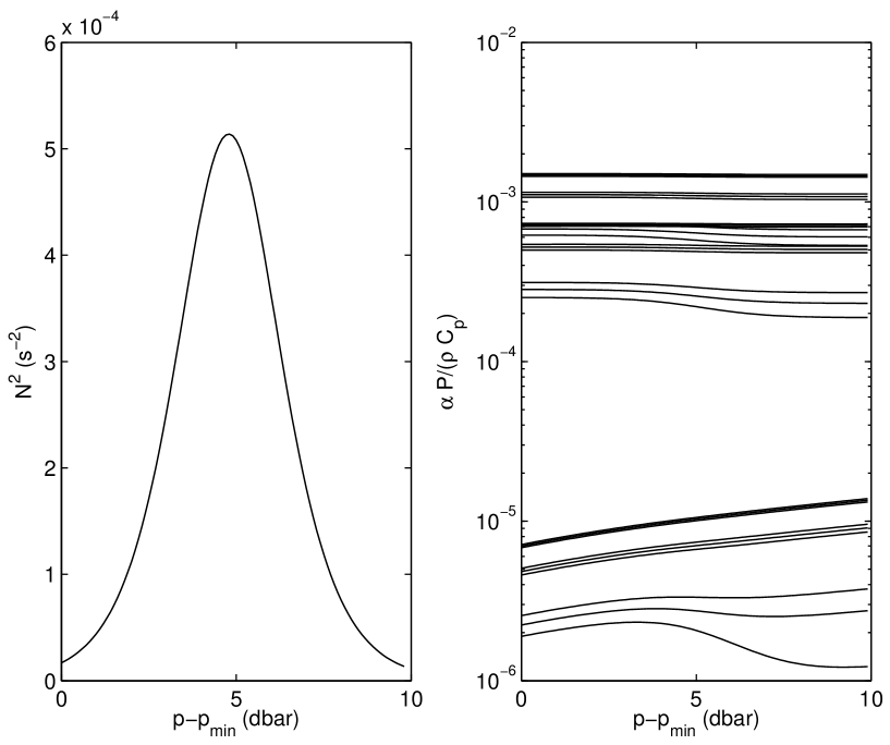
Abbildung 2: (Top panel) The squared buoyancy frequency $N^{2}$ common to all stratifications considered. (Bottom panel) The thermodynamic efficiency-like quantity $\alpha P/(\rho C_{p})$ corresponding to the 27 different cases considered. Note that the Fofonoff regime, i.e., the case for which $GPE$ decreases as the result of mixing, is expected whenever the latter quantity decreases for increasing pressure. The classical case considered by the literature, i.e., the case for which $GPE$ increases as the result of mixing corresponds to the case where the latter quantity increases with increasing pressure on average (see Table 1 for more details).

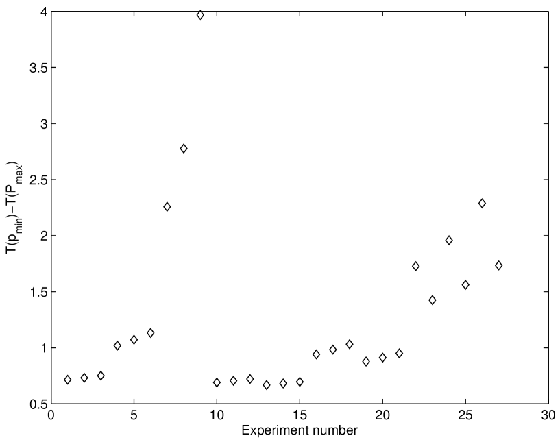
Abbildung 3: Distribution of the top-bottom temperature difference $T(P_{min})-T(P_{max})$ as a function of the experiment number.

f

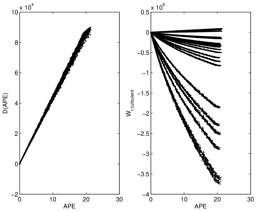
Abbildung 4: (Left panel) The dissipation rate of $APE$ as a function of $APE$, each point corresponding to one particular experiment. Note that there is no obvious dependence on the stratification. (Bottom panel) The rate of change $W_{r,turbulent}$ as a function of $APE$. This time, each stratification is associated with a different curve.

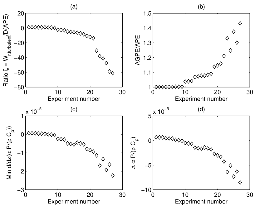
Abbildung 5: (a) The averaged ratio $\xi=W_{r,turbulent}/D(APE)$ as a function of the experiment number; (b) The averaged ratio $AGPE/APE$ as a function of the experiment number; (c) The minimum value of $d/dz[\alpha P/(\rho C_{p})$ as a function of the experiment number; (d) The top-bottom difference of $\alpha P/(\rho C_{p})$ as a function of the experiment number.

t

Tabelle 1: Averaged values of the two ratios $\xi=W_{r,turbulent}/D(APE)$ and $AGPE/APE$ for the 27 different types of stratifications considered in this paper. The quantities $[d\Upsilon/dz]_{min}$ and $\Delta\Upsilon$ refer to the minimum value of the vertical derivative of $\Upsilon=\alpha P/(\rho C_{p})$ and top-bottom difference of $\Upsilon$ respectively. $S$ is the salinity used in the equation of state for seawater, $\overline{T}$ is the mean temperature of the profile considered, and $P_{min}$ denotes the minimum value of the vertical pressure profile. The top-bottom temperature differences are displayed in Fig. 3, while the pressure interval is $10\,{\rm dbar}$ in all cases. The tabulated values demonstrate that increasingly negative values of $\xi$ coincide with increasingly large positive values of $d\Upsilon/dz$, as well as with with the increasing importance of non-Boussinesq compressible effects associated with an increasing discrepancy between $AGPE$ and $APE$. The standard case for which $\xi\approx 1$ is achieved close to atmospheric pressure. The maximum negative value of $\xi$ occurs for the lowest $S$, lowest $\overline{T}$, and largest $P_{min}$ values considered.

Expt	$\xi$	$AGPE/APE$	$[d\Upsilon/dz]_{min}\times 10^{6}$	$\Delta\Upsilon\times 10^{6}$	S(psu)	$\overline{T}(^{\circ}C)$	$P_{min}(dbar)$
1	0.98	1.0003	-6.70	-0.64	40	22.6	0
2	0.98	1.0003	-6.53	-0.63	35	22.6	0
3	0.98	1.0003	-6.36	-0.61	30	22.6	0
4	0.95	1.0005	-4.50	-0.40	40	12.5	0
5	0.95	1.0005	-4.23	-0.37	35	12.5	0
6	0.94	1.0006	-3.95	-0.33	30	12.4	0
7	0.71	1.0015	-1.20	0.03	40	1.9	0
8	0.55	1.0018	-0.51	0.15	35	1.6	0
9	0.10	1.0026	0.67	0.35	30	1.2	0
10	-2.41	1.0369	5.07	2.42	40	22.6	1000
11	-2.67	1.0391	5.89	2.61	35	22.6	1000
12	-2.96	1.0416	6.76	2.81	30	22.6	1000
13	-4.93	1.0682	14.42	4.87	40	22.7	2000
14	-5.36	1.0724	15.72	5.18	35	22.7	2000
15	-5.84	1.0768	17.09	5.51	30	22.6	2000
16	-6.35	1.0772	14.05	4.44	40	12.5	1000
17	-7.35	1.0835	15.97	4.89	35	12.5	1000
18	-8.53	1.0905	18.10	5.40	30	12.5	1000
19	-10.73	1.1372	27.10	7.87	40	12.6	2000
20	-12.17	1.1476	30.02	8.58	35	12.5	2000
21	-13.86	1.1591	33.23	9.37	30	12.5	2000
22	-30.73	1.2109	42.67	11.36	40	2.1	1000
23	-38.06	1.3306	63.86	16.93	40	2.3	2000
24	-41.26	1.2482	51.06	13.42	35	2.0	1000
25	-47.46	1.3751	73.20	19.26	35	2.2	2000
26	-58.84	1.3010	63.09	16.37	30	1.9	1000
27	-61.06	1.4318	85.31	22.28	30	2.1	2000