Conductance distribution in two-dimensional localized systems with and without magnetic fields

Abstract

We have obtained the universal conductance distribution of two-dimensional disordered systems in the strongly localized limit. This distribution is directly related to the Tracy-Widom distribution, which has recently appeared in many different problems. We first map a forward scattering paths model into a problem of directed random polymers previously solved. We show numerically that the same distribution also applies to other forward scattering paths models and to the Anderson model. We show that most of the electric current follows a preferential percolation-type path. The particular form of the distribution depends on the type of leads used to measure the conductance. The application of a moderate magnetic field changes the average conductance and the size of fluctuations, but not the distribution when properly scaled. Although the presence of magnetic field changes the universality class, we show that the conductance distribution in the strongly localized limit is the same for both classes.

1 Introduction

The hypothesis of single-parameter-scaling (SPS) T74 ; AA79 constitutes the main foundation of our understanding of localization in disordered systems. The original formulation of the SPS hypothesis focused on the average conductance, but it was soon realized that the full distribution function of the conductance should be considered. Then, according to the SPS hypothesis, the conductance distribution function should depend on a single parameter shapiro , for example, the mean conductance $\langle g\rangle$ or the mean of the logarithm, $\langle\ln g\rangle$.

The validity of the SPS hypothesis has been thoroughly checked in one–dimensional (1D) systems, where it has been shown that all the cumulants of $\ln g$ scale linearly with system size Ro92 . Thus, the distribution function of $\ln g$ approaches a Gaussian form for asymptotically long systems, which in 1D are always strongly localized. It is fully characterized by two parameters, the mean $\langle\ln g\rangle$ and the variance $\sigma^{2}$ of $\ln g$. In the scaling regime, both parameters are related to each other through a universal law,

$$\frac{\sigma^{2}\xi}{2L}=1$$ (1)

where $L$ is the system size and $\xi$ the localization length, defined as

$$\xi=-\lim_{L\to\infty}\frac{2L}{\langle\ln g\rangle}\,.$$ (2)

Eq. (1) was first derived in Ref. At80 within the so–called random phase hypothesis, which assumes that there exists a microscopic length scale over which phases of complex transmission and reflection coefficients become completely randomized. This relation reduces the two parameters of the distribution to only one and provides, therefore, a justification and interpretation for SPS in 1D systems.

The situation in higher dimensional systems is not as clear as in 1D systems. In those dimensions is far more difficult to do analytical calculations and numerical simulations have been limited until recently to small sample sizes. In the diffusive regime, although the size of universal conductance fluctuations depend on the dimension of the system, the distribution function of the conductance tends to a gaussian for all dimensions. Some people thought that in the localized regime it could happen something similar. In the strong localization regime, $\ln g$ was claimed to be normally distributed in dimensions higher than one CM87 ; KK92 ; KM93 . However, it was pointed out that the distribution is not log-normal Ma02 ; MM04 ; MM05 ; PS06 . We found numerically that the variance behaves as PS05 ; SP06

$$\sigma^{2}=A\langle-\ln g\rangle^{\alpha}+B$$ (3)

with the exponent $\alpha$ equal to $2/3$ in two-dimensional (2D) systems. In three-dimensional systems, preliminary results indicated a possible value of $\alpha=2/5$ SP06 , but recent more extensive simulations point out to a value of $1/2$, in agreement with directed polymer simulations KM91 . The constants $A$ and $B$ are model or geometry dependent. The precise knowledge of the dependence of $\sigma^{2}$ with $\langle-\ln g\rangle$ made much easier the numerical verification of the SPS hypothesis, which we checked for the Anderson model PS05 .

In this paper, we concentrate in the strongly localized regime in 2D systems. Although experimental measurements of coherent transport at low temperatures are difficult in this regime, knowledge of the conductance distribution is of interest to better understand variable range hopping conductance, the metal-insulator transition in three dimensions or the crossover between the diffusive and the localized regime in 2D systems.

In the strongly localized regime, the contribution of each Feynman path to the tunneling amplitude between two sites decays exponentially with its distance, and we can expect that some properties of the conductance (in particular the size dependence) should be dominated by the shortest or forward-scattering paths (FSP). This approach was introduced by Nguyen, Spivak and Shklovskii (NSS) NS85 in a model to account for quantum interference effects in the localized regime. Medina and Kardar MK92 studied in detail the model. They computed numerically the probability distribution for tunneling and found that it is approximately log-normal, with its variance increasing with distance as $r^{2/3}$ for 2D systems. This is in contrast with the 1D case, where the variance grows linearly with distance, and with the implicit assumptions of some works on 2D systems. In our opinion, this approximation did not receive as much attention as it deserves, probably because in the SPS regime the localization length must be much larger than the lattice constant, which means that contributions from other paths cannot be negligible.

A major step forward in the field of random systems was done by Tracy and Widom (TW) TW who obtained the distribution function of the largest eigenvalue of random matrices belonging to the gaussian ensembles, orthogonal, unitary and symplectic. It soon became clear that the TW distribution for the unitary ensemble also appears in the calculation of the length of the longest common subsequence in a random permutation BD99 and in many other seemingly unrelated problems. For an introduction see Ref. majundar . Particularly important for our problem is the study by Johansson Johansson of a specific type of directed polymer model. He obtained the distribution function of the lowest energy state exactly in terms of the Tracy-Widom (TW) distribution. Also relevant for us is the one-dimensional polynuclear growth model png , which studies the height fluctuations of a growing interface and is closely related to the Kardar-Parisi-Zhang equation KPZ .

We showed that for the 2D Anderson model in the strongly localized limit the conductance distribution is related to the TW distribution SO07 . Here we present results for two different models in the FSP approximation, which is important to link exact results in directed polymers with the more realistic Anderson model. We show numerically that for a model with disorder with both positive and negative values (which cannot be exactly mapped to the solvable model) the skewness of the conductance distribution tends without free parameters the TW value. The role of percolation versus interference is also analyzed. We finally study the conductance distribution function in the presence of a magnetic field. We show that systems in the orthogonal gaussian ensemble (Anderson model without magnetic field) and in the unitary gaussian ensemble. (Anderson model with magnetic field) tend to the same behavior in the strongly localized limit.

In the next section, we describe the two models that we have used in our calculations. In section III, we present a mapping of the conductance in localized systems to the free energy of directed polymers and use Johansson’s results to get the distribution function. In sections IV and V, we show that the distribution function of the logarithm of the conductance in the FSP approximation and in the Anderson model, respectively, are related to the TW distribution. In section VI, we analyze the effects of a magnetic field. We finalize with a discussion and conclusion section.

2 Model

We have studied numerically the Anderson model and its FSP approximation for 2D samples. For the Anderson model, we consider square samples of size $L\times L$ described by the standard Anderson Hamiltonian

$$H=\sum_{i}\epsilon_{i}a_{i}^{\dagger}a_{i}+t\sum_{i,j}a_{j}^{\dagger}a_{i}+{\rm h.c.}\;,$$ (4)

where the operator $a_{i}^{\dagger}$ ($a_{i}$) creates (destroys) an electron at site $i$ of a cubic lattice and $\epsilon_{i}$ is the energy of this site chosen randomly between $(-W/2,W/2)$ with uniform probability. The double sum runs over nearest neighbors. The hopping matrix element $t$ is taken equal to $-1$, which set the energy scale, and the lattice constant equal to 1, setting the length scale. All calculations with the Anderson model are done at an energy equal to 0.01, to avoid the center of the band.

We have calculated the zero temperature conductance $g$ from the Green functions. The conductance $g$ is proportional to the transmission coefficient $T$ between two semi–infinite leads attached at opposite sides of the sample

$$g=\frac{2e^{2}}{h}T$$ (5)

where the factor of 2 comes from the spin. ¿From now on, we will measure the conductance in units of $2e^{2}/h$. The transmission coefficient can be obtained from the Green function, which can be calculated propagating layer by layer with the recursive Green function method M85 ; V98 . This drastically reduces the computational effort. Instead of inverting an $L^{2}\times L^{2}$ matrix, we just have to invert $L$ times $L\times L$ matrices. With the iterative method we can easily solve square samples with lateral dimension up to $L=400$. We have considered ranges of disorder $W$ equal to 13, 15 and 25, which correspond to localization lengths of 1.12, 2.4 and 3.2, respectively, and lateral dimensions up to $L=200$ for the calculation of the distribution function, which requires a huge number of independent runs to get good statistics in the tails. For this purpose, we average over a number of realizations larger than $6\times 10^{5}$ for each disorder and size. The leads serve to obtain the conductivity from the transmission formula in a way well controlled theoretically and close to the experimental situation.

To consider different possible geometries, we have used two types of leads: wide leads with the same width as the lateral dimension of the samples and narrow (one-dimensional) leads. These are attached to the sample at the centers of opposite edges, as shown in Fig 1(a). The scheme of the wide leads is shown in Fig 1(b). In both cases the leads are represented by the same hamiltonian as the system, Eq. (4), but without diagonal disorder. The narrow leads can be viewed as a simplified model of a point contact, while the wide leads should roughly correspond to electrodes in contact with the whole edge of the sample. We use cyclic periodic boundary conditions in the direction perpendicular to the leads.

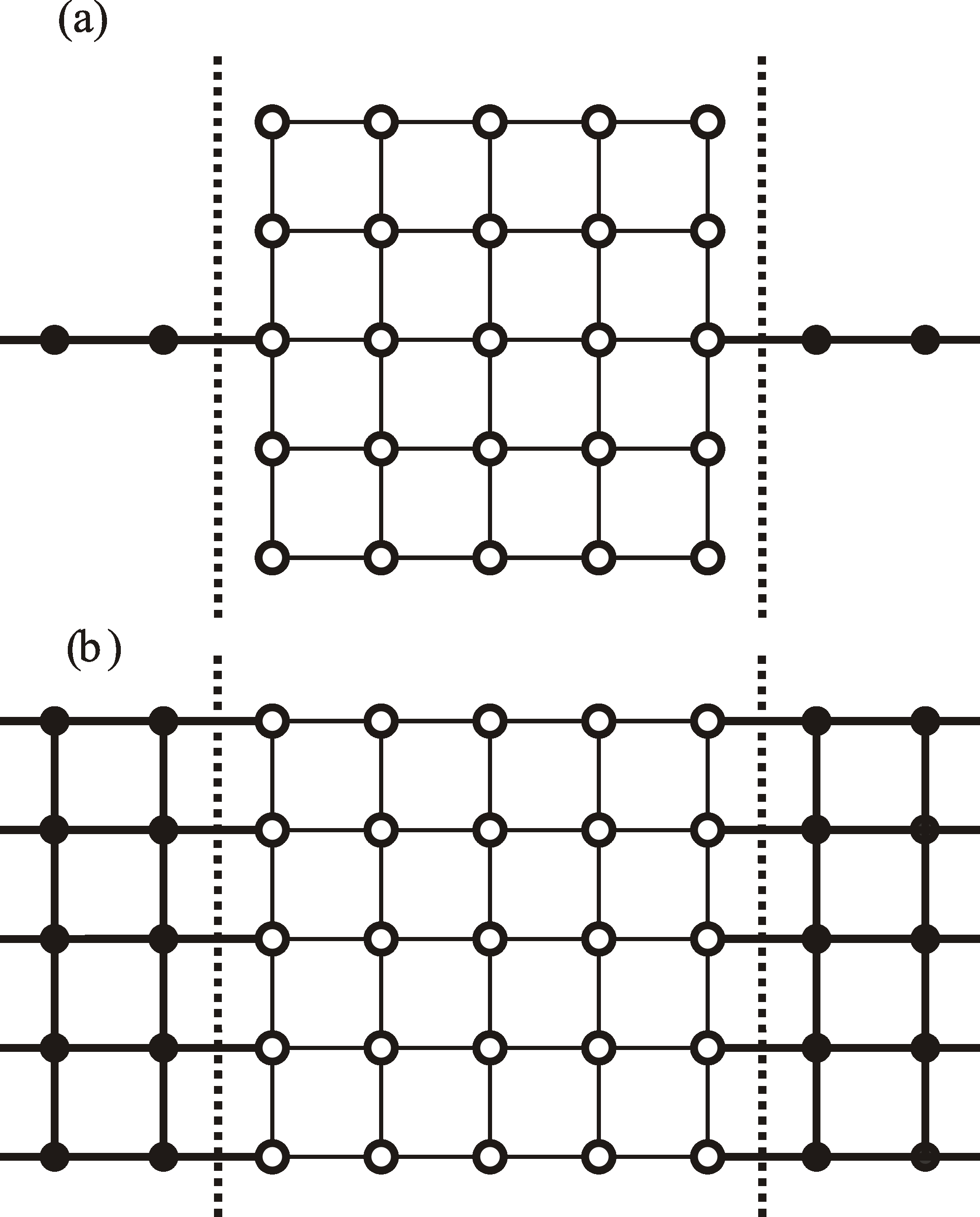
Figure 1: Schematic picture of the sample and the leads considered: (a) narrow leads and (b) wide leads. The open circles represent sites in the system and the solid dots sites in the leads. The lines represent the hopping between sites. The dashed lines are just a guide to the eye.

The introduction of a uniform magnetic field $B$ perpendicular to the sample leads to complex hopping matrix elements. In the Landau gauge the vector potential is $\mathbf{A}=(0,-Bx,0)$. Then, the hopping matrix elements in the $X$ direction are unchanged by the presence of the field, while the elements in the $Y$ direction have to be multiplied by the factor $\exp(\pm ixB)$, where the sign depends on whether we are connecting a site with the upper or lower site in the same column SB84 .

We have also studied the FSP approximation, first considered by Nguyen, Spivak and Shklovskii NS85 and widely studied by Medina and Kardar MK92 in 2D square samples. One can write the matrix elements of the Green function between two sites $a$ and $b$ in terms of the locator expansion

$$\langle a|G|b\rangle=\sum_{\Gamma}\prod_{i\in\Gamma}\frac{1}{E-\epsilon_{i}}\;,$$ (6)

where the sum runs over all possible paths connecting the two sites $a$ and $b$. In general the convergence of this series is very problematic, but in the strongly localized regime for distances much larger than the localization length one expect that the previous sum is dominated by the FSP. Considering only directed paths is well justified in the strongly localized regime, where the contribution of each trajectory is exponentially small in its length. We expect that back-scattering paths renormalize the site energies, but they should be irrelevant in the renormalization-group sense in the strongly localized regime. Based on this idea, the FSP approximation only considers directed paths. In this approximation, we will consider $E=0$ and two types of diagonal disorder: i) $\epsilon_{i}$ can only take two values $W$ and $-W$, chosen at random with the same probability, which was the model originally considered in Ref. NS85 ; ii) $\epsilon_{i}=\max[|x|,1]{\rm sign}(x)$, where $x$ is chosen randomly in the interval $(-W/2,W/2)$ with uniform probability. The reason to substitute the small disorder energies, $|\epsilon_{i}|<1$ by $\pm 1$ is to take partially into account the effects of backward paths, which for these sites are important, avoiding at the same time problems of convergence in the locator expansion and ensuring that the transmission through any path is never larger than one. We will refer as NSS model to the FSP approximation with the first type of disorder. For the FSP approximation, we concentrate on the transmission amplitude between two points in opposite corners of a square sample and we assume that the quantum trajectories joining these two points have to follow one of the (many) shortest possible paths. For the NSS model it is standard to use the path length $l$, rather than the system size $L$. For our geometry, $l=2L$. The transmission at zero energy is equal to MK92

$$T=\left(\frac{2t}{W}\right)^{2l}J^{2}(l)\;,$$ (7)

where the transmission amplitude $J(l)$ is given by the sum over all the directed paths

$$J(l)=\sum_{\Gamma}^{\rm directed}J_{\Gamma}\;,$$ (8)

The contribution of each path, $J_{\Gamma}$, is the product of the signs of the disorder along the path $\Gamma$. $J$ does not depend on $W$ for the first type of disorder and only weakly for the second type, for which we take $W=10$.

The variance of $\ln g$ is entirely determined by $J^{2}(l)$ and so it depends on $l$. It is convenient to quantify the magnitude of the fluctuations in terms of the path length $l$ in the FSP approximation. $\langle\ln g\rangle$ is, of course, proportional to $l$, but the constant of proportionality depends on the disorder $W$. The assumption of directed paths facilitates the computational problem and makes feasible to handle system sizes much larger than with the Anderson hamiltonian. The sum over the directed paths can be obtained propagating layer by layer the weight of all the trajectories in a very efficient way MK92 .

3 Mapping of the conductance in localized systems to polymers

We have proven that for a specific FSP model the distribution function of the logarithm of the conductance in 2D systems is a Tracy-Widom distribution. To do so, we have to map the problem of the conductance in strongly localized systems to the problem of finding the energy of a polymer in a random environment. Each FPS path contributing to the conductance corresponds to a directed polymer. The calculation of the quantum amplitude between two points, given by Eq. (6), in the FSP approximation is then formally similar to the calculation of the partition function of directed polymers in a random potential at a very small temperature $T=1/k\beta$

$$Z=\sum_{\Gamma}\exp\left\{-\beta\sum_{i\in\Gamma}h_{i}\right\}=\;,\sum_{\Gamma}\prod_{i\in\Gamma}\exp\left\{-\beta h_{i}\right\}$$ (9)

$h_{i}$ are random site energies and $\Gamma$ runs over all possible configurations of the directed polymer. We can easily make Eqns. (6) and (9) equivalent by associating $\beta h_{i}$ with $\ln(E-\epsilon_{i})$. In this case, we can map the distribution of $\ln g$ in our system to the distribution of the free energy in directed polymers. As in polymer physics we consider real disorder energies $h_{i}$, we then choose all the values $E-\epsilon_{i}$ to be positive.

The distribution function of the ground state energy $H$ of a polymer in a disordered environment was obtained exactly by Johansson Johansson . In his model the random site energies take integer values with probabilities ${\rm Pr}(h_{i}=k)=(1-p)p^{k}$. The ground state energy for polymers running between the origin and the point $(x,y)$ is given by Johansson

$$H(x,y) \rightarrow \frac{2\sqrt{pxy}+p(x+y)}{1-p}$$

$$+ \frac{(pxy)^{1/6}}{1-p}\left[(1+p)+\sqrt{\frac{p}{xy}}(x+y)\right]^{2/3}\chi_{2}$$

where $\chi_{2}$ is a random variable with the TW distribution, corresponding to the distribution of the largest eigenvalue of a complex hermitian random matrix TW . $\chi_{2}$ verifies

$${\rm Pr}(\chi_{2}<x)=\int_{\infty}^{x}f_{2}(x^{\prime})dx^{\prime}=e^{-g(x)}$$ (11)

where $g(x)$ is the solution of the equation

$$g^{\prime\prime}(x)=u^{2}(x),$$ (12)

which tends to zero, $g(x)\rightarrow 0$, as $x\rightarrow\infty$. $u(x)$ is the global positive solution of the Painlevé II equation

$$u^{\prime\prime}=2u^{3}+xu$$ (13)

which tends to the Airy function, $u(x)\rightarrow{\rm Ai}(x)$, when $x\rightarrow\infty$.

We can map Johansson’s result for the polymer problem to obtain the distribution function of the conductance for the localization problem by considering the FSP approximation and that the disorder energies are of the form

$$\epsilon_{i}=E+e^{\beta k}$$ (14)

with probability ${\rm Pr}(k)=(1-p)p^{k}$ for $k=0,1,2,\cdots$, in the limit $\beta\rightarrow\infty$. This is a very specific model, but we expect that their results apply in a much more general context, i.e., different disorder probabilities, as already suggested by Johansson Johansson . The same distribution should also apply for non zero temperature, as in a renormalization-group sense temperature is an irrelevant parameter and the behavior is dominated by the zero-temperature fixed point.

It is not trivial to extend the previous mapping to realistic problems with negative site energies, like the NSS and the Anderson model. It is then natural to study if the distribution function given by Eq. (3) also applies to these models.

4 Conduction in the forward scattering paths approximation.

First of all, we have studied the conductance distribution of the NSS model in order to check if it is also given by the TW function. For this model it is natural to consider $\ln J^{2}$, which contains all the relevant information about fluctuations. In Fig. 2 we plot, for several system sizes, histograms of $\ln J^{2}$ as a function of $z=(\ln J^{2}-\langle\ln J^{2}\rangle)/\sigma$, where $\sigma^{2}$ is the variance of $\ln J^{2}$. The data are for narrow leads and each line corresponds to a different system size, specified in the figure. The thick solid line is the standardized TW distribution. We see how the results for the NSS model tend uniformly to the TW distribution as size increases, although the convergence is relatively slow.

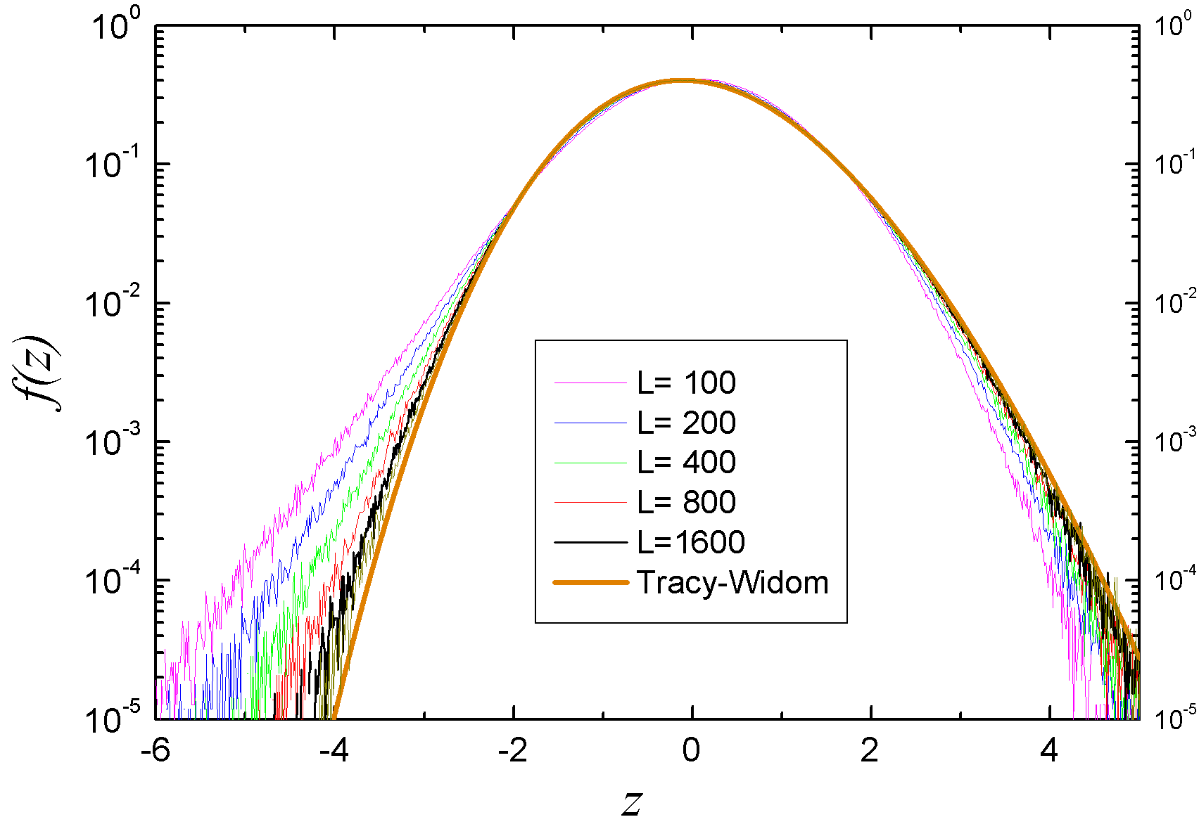
Figure 2: Histograms of $\ln J^{2}$ as a function of the standardized variable $z$ for several sizes of the NSS model. The thick solid line corresponds to the TW distribution. As size increases, the data approach the TW distribution.

Although the results in Fig. 2 present noticeable finite size effects, it is clear that the TW distribution is fully consistent with the limiting distribution. This fact together with the previous mapping permit us to suggest that

$$\ln J^{2}=\alpha L+\beta L^{1/3}\chi_{2}$$ (15)

in the limit $L\rightarrow\infty$. To better guarantee that the TW distribution is the proper limiting function, it is convenient to focus on the adimensional parameters of the distribution, like the skewness (${\rm Sk}=k_{3}/k_{2}^{3/2}$) or the kurtosis (${\rm Kur}=k_{4}/k_{2}^{2}$). If the previous equation is correct, these two parameters must tend to the TW values as $L\rightarrow\infty$ independently of the values of $\alpha$ and $\beta$. From Eq. (15) we expect that the leading correction for the skewness, with respect to the limiting value at $L\rightarrow\infty$, is proportional to $L^{-2/3}$. In Fig. 3 we plot the skewness as a function of $L^{-2/3}$ for the NSS model (circles) and for our second FSP model, with continuous disorder (triangles). The horizontal line corresponds to the TW value. We see how the skewness approaches the correct value and how it does so in the expected way for the two FSP models considered. Finite size effects for the NSS model are larger than for the other FSP model considered. A similar behavior is also observed for the kurtosis. It is clear from these trends that both models tend to the same universal distribution.

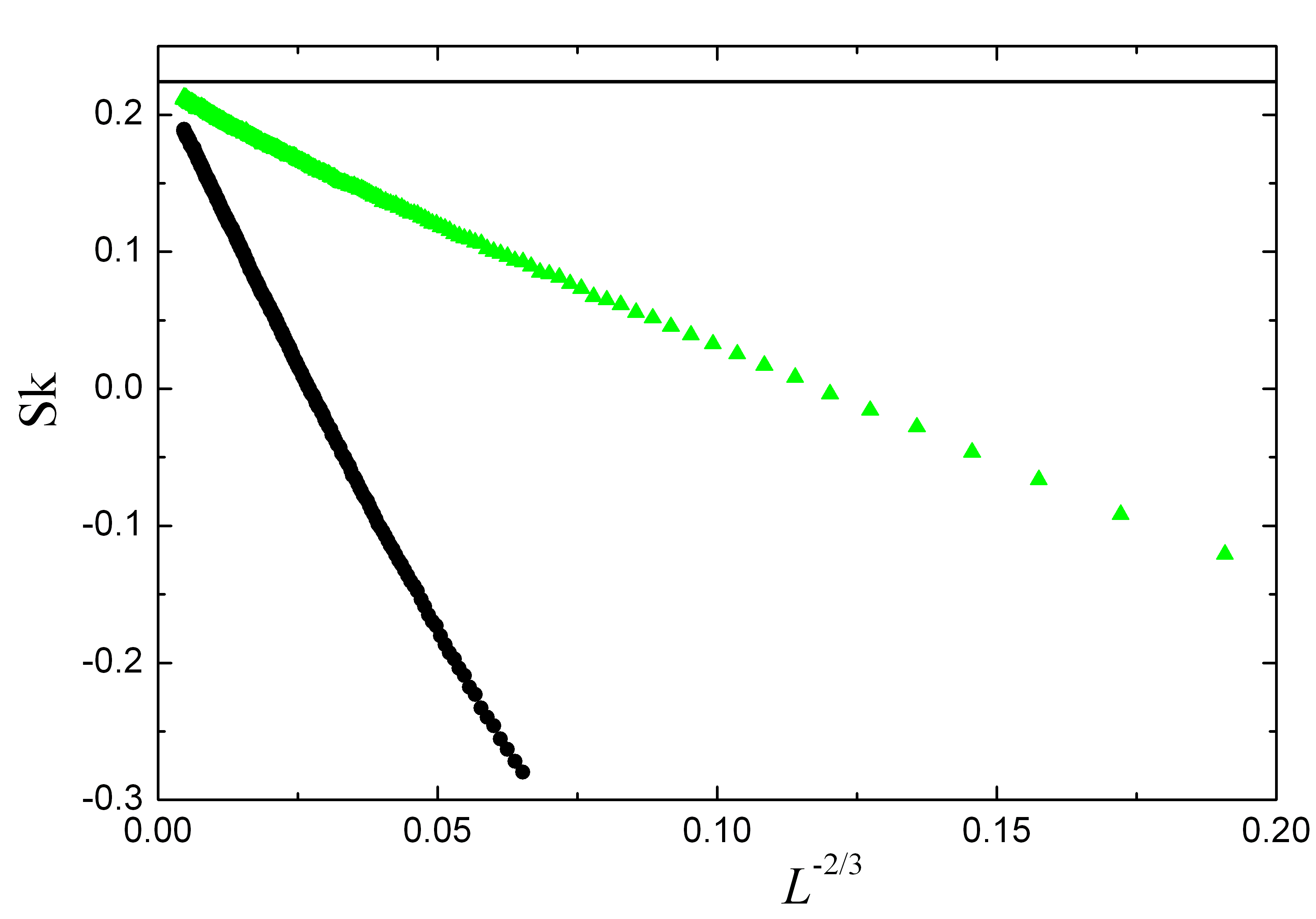
Figure 3: Skewness vs $L^{-2/3}$ for the NSS model (black circles) and the FSP approximation with continuous disorder (green triangles). The horizontal line corresponds to the TW value.

We note that Johansson’s results imply that the conductivity, in our case, is likely to be dominated by the most important FSP. On the contrary, the NSS model was designed to maximize the interference effects and all trajectories have the same amplitude. So, considering only the most conducting path has no sense in this case. It is necessary then to understand how the NSS may end up reproducing the TW distribution. In Fig. 4 we plot, for a given sample, the value of $J^{2}$ from the left corner to any other point in the sample. All points in a vertical slice are at the same hopping distance from the left corner. For each vertical slice the maximum value of $J^{2}$ is plotted in black and the minimum in white. Intermediate values are plotted on a gre y scale proportional to $J^{2}$. This method gets rid of the exponential decay of $J^{2}$ with distance. However, it does not take into account that the current must flow through the end point. Despite the fact that all single trajectories have exactly the same weight, interference effects produce that most of the current is carried through very few well defined paths. The interference effects play a role only at short scales, producing a kind of renormalization process, which ends up in a dominant “renormalized” path. Probably, this renormalization also explains why finite size effect are larger in the NSS model than in the other FSP model considered.

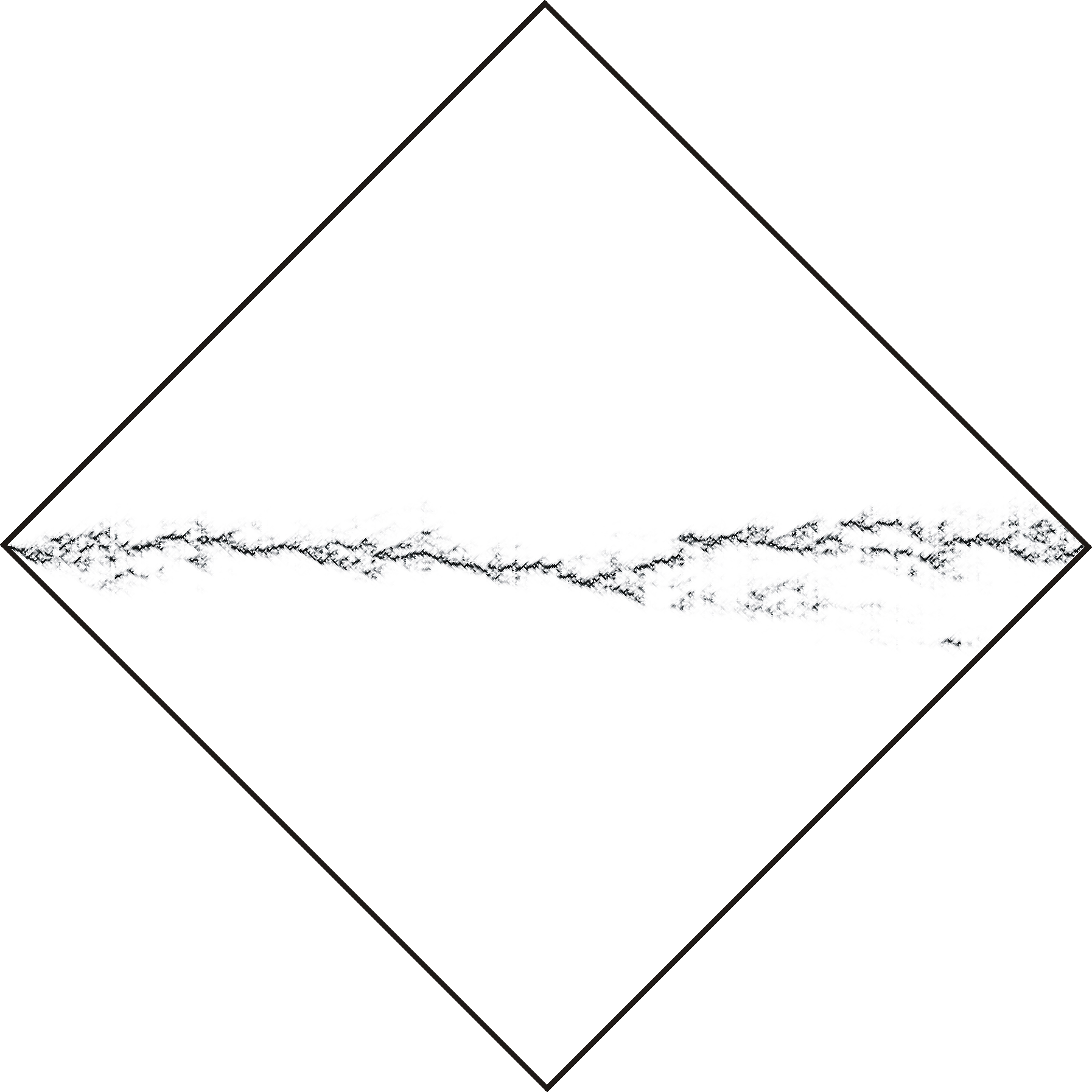
Figure 4: Plot of $J^{2}$ from the left corner to any other point in a given sample on a grey scale. On each vertical slice, black (white) corresponds to the maximum (minimum) conductance.

5 Conductance for the Anderson model

Once we have shown that the conductance in the FSP approximation follows the TW distribution, we study the Anderson model, which cannot be directly mapped to the polymer problem. We have calculated numerically the conductance for the 2D Anderson model and we have obtained its distribution function. By similarity with the FSP models we first consider the narrow leads geometry. In Fig. 5 we plot histograms of $\ln g$ for this model as a function of $\chi=(\ln g-A)/B$, where $A$ and $B$ are chosen in order to have the same mean and variance as the theoretical distribution, the TW distribution $f_{2}(\chi_{2})$. The data are for several sizes and ranges of the disorder, $W=25$ and $L=100$ (squares), $W=13$ and $L=200$ (dots), $W=15$ and $L=150$ (triangles) and $W=9$ and $L=70$ (connected circles). The solid line corresponds to $f_{2}(\chi_{2})$. All the cases in the strongly localized regime, represented by unconnected solid symbols, are fitted fairly well by $f_{2}(\chi_{2})$. The agreement extends over more than four orders of magnitude. The connected empty circles correspond to a system near the crossover regime, whose distribution is close to a log-normal, represented by a dashed line in Fig. 5. For narrow leads, $f_{2}(\chi_{2})$ fits the data better than the gaussian function for $L/\xi\gtrsim 13$.

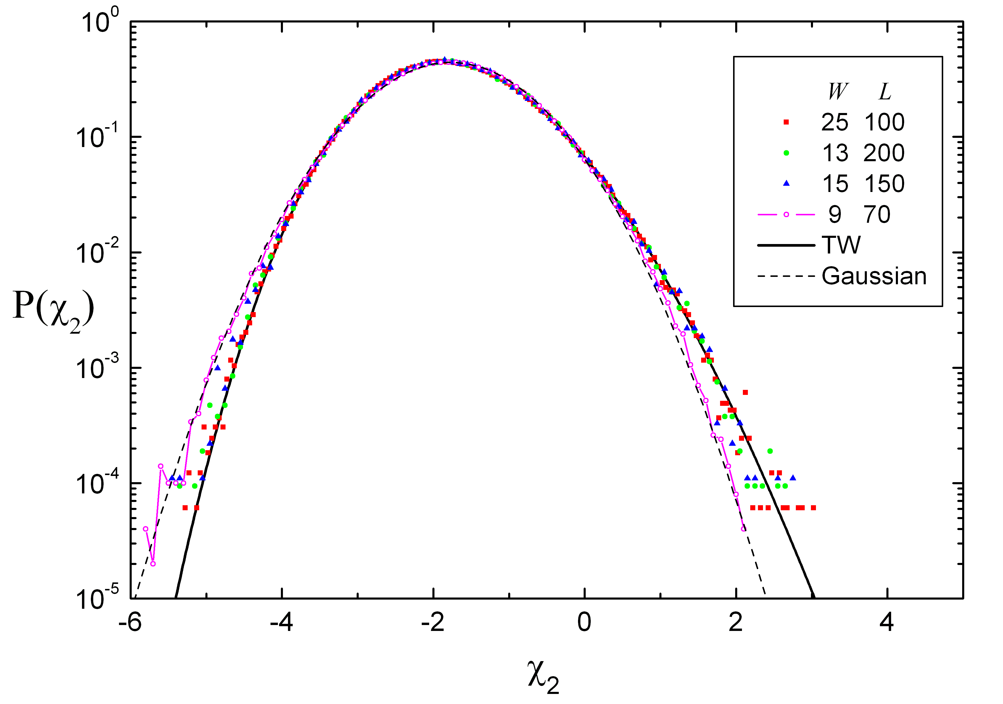
Figure 5: Histograms of $\ln g$ versus the scaled variable $\chi$ for several sizes and disorders of the Anderson model with narrow leads. The continuous line corresponds to the TW distribution and the dashed line is a gaussian with the same mean and variance as the TW distribution.

Considering the size dependence of the mean and the variance of $\ln g$ and the excellent agreement between our data and the TW distribution, we conclude that in the strongly localized regime with narrow leads

$$\ln g=-\frac{2L}{\xi}+\beta\left(\frac{L}{\xi}\right)^{1/3}\chi_{2}$$ (16)

where $\beta$ is a new constant and $\chi_{2}$ a random variable with the TW distribution. In the SPS regime $\beta$ is a constant, independent of the disorder, the system size or the Fermi energy. We found, from present results and previous calculations on the behavior of the variance, that it is approximately equal $3.4$ for the Anderson model with narrow leads. Eq. (16) must be also valid outside the SPS regime (when the localization length is very small or when the Fermi energy lies in the band tails), but with a non universal value of $\beta$. The data set in Fig. 5 for $W=25$ is outside the SPS regime, since it corresponds to a localization length of the order of the lattice spacing ($\xi=0.97$), and fits the TW distribution very well. The value of $\beta$ is 3.5 in this case.

Table 1: Mean, variance, skewness, and kurtosis for the distributions $f_{2}$ and $f_{0}$.

	$f_{2}$	$f_{0}$
Mean	-1.77109	0
Variance	0.81320	1.15039
Skewness	0.2241	0.35941
Kurtosis	0.09345	0.28916

In table I we present the characteristic parameters of the distribution of $f_{2}(\chi_{2})$. The fact that it has a mean different from zero, $\langle\chi_{2}\rangle=-1.77109$, has some practical consequences. According to Eq. (16), this implies a contribution to $\langle\ln g\rangle$ proportional to $L^{1/3}$, already observed by us PS06 in the Anderson model with narrow leads. This is of practical interest for the calculation of the localization length. Neglecting this term can cause errors of the order of 20 % in the estimate of the localization length.

We did not find any $L^{1/3}$ contribution for wide leads, which constitutes a strong indication that the conductance distribution may depend on the leads, even in the strongly localized regime. The type of leads may change the universality class. We can expect a situation similar to polynuclear growth models png , where the height distribution was found to depend on the initial conditions. Our problem with narrow leads is directly related to the droplet model in Ref. png , which starts from an initial preferential point. With wide leads we have translational invariance and all the initial (and final) points are equivalent, a problem similar to stationary growth. In this case, the height fluctuations are described by the function $f_{0}$ whose accumulated distribution is png

$$\int_{\infty}^{x}f_{0}(x^{\prime})dx^{\prime}=\left[1-(x+2f^{\prime\prime}+2g^{\prime\prime})g^{\prime}\right]e^{-(g+2f)}$$ (17)

where $f(x)$ is the solution of the equation

$$f^{\prime}(x)=-u(x),$$ (18)

which tends to zero when $x\rightarrow\infty$. $g(x)$ and $u(x)$ are given by Eqs. (12) and (13), respectively. The characteristic parameters of the distribution $f_{0}$ are given in table I. As required by our previous finding that there were no $L^{1/3}$ contributions to $\langle\ln g\rangle$, $f_{0}$ has zero mean. In Fig 6 we show the histograms of $\ln g$ for the Anderson model with wide leads for several disorders and sizes, $W=13$ and $L=100$ (squares), $W=13$ and $L=200$ (dots), $W=15$ and $L=100$ (triangles) and $W=10$ and $L=50$ (connected circles). The solid symbols correspond to systems in the strongly localized regime, while connected empty symbols to a case near the crossover. We plot in terms of $\chi=(\ln g-A)/B$, where $A$ and $B$ are chosen in order to have the same mean and variance as the distribution $f_{0}$. The full line corresponds to $f_{0}$ and the dashed line to a gaussian with the same mean and variance. The agreement between the numerical data and the theoretical distribution is again excellent, showing that $\ln g$ satisfies in this case

$$\ln g=-\frac{2L}{\xi}+\beta\left(\frac{L}{\xi}\right)^{1/3}\chi_{0}$$ (19)

where $\beta$ is a new constant and $\chi_{0}$ a new random variable with distribution $f_{0}(x)$. In the SPS regime, $\beta$ is a universal constant approximately equal to 2.2. We note that, in the data for $W=10$ and $L=50$, the right tail of the distribution is cut at $\chi_{0}\approx 4$. This is due to the existence of a kink in the distribution for a transmission equal to one. For wide leads the distribution $f_{0}(\chi_{0})$ fits the data well when $L/\xi\gtrsim 6$.

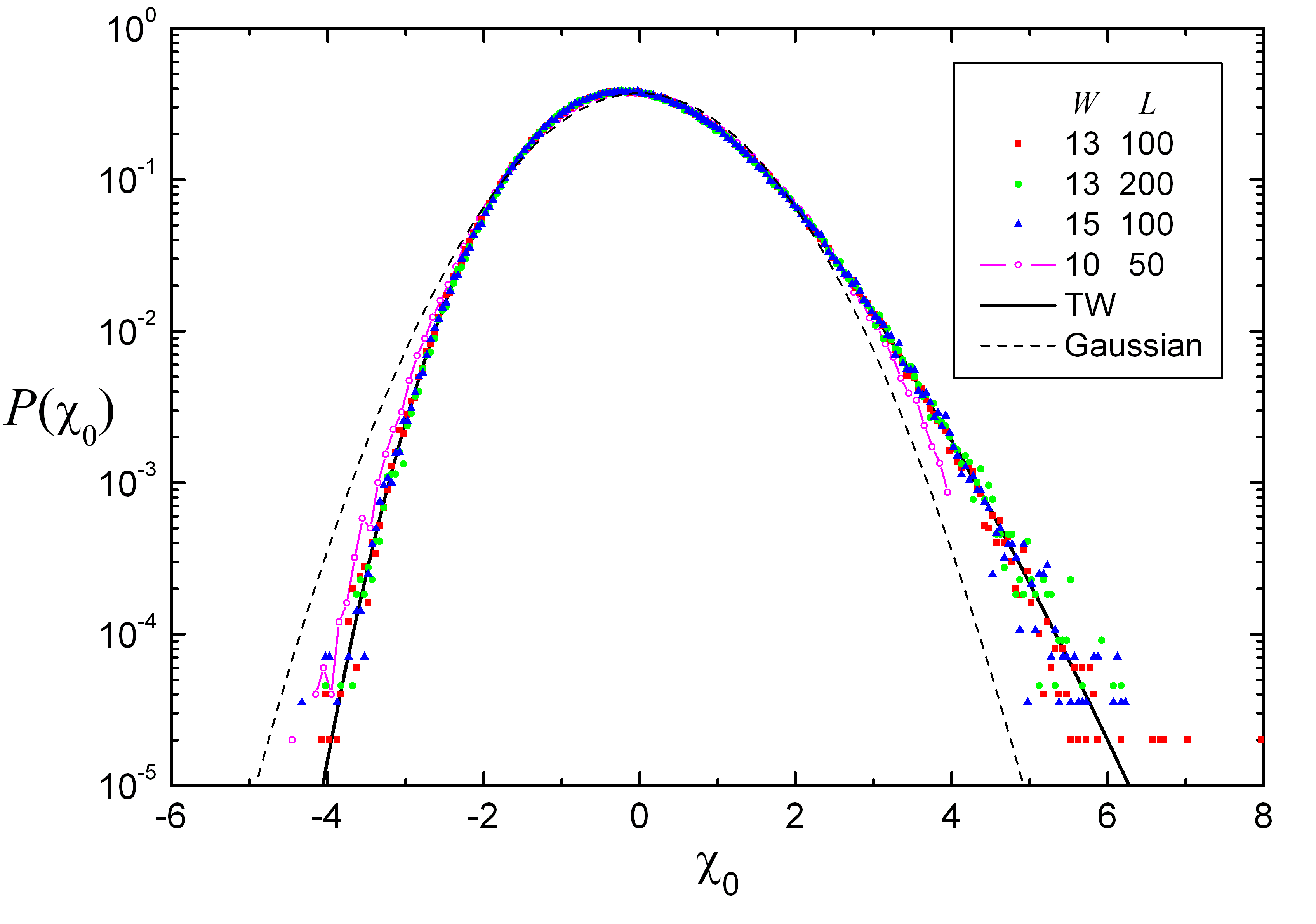
Figure 6: Histograms of $\ln g$ versus the scaled variable $\chi$ for several sizes and disorders of the Anderson model with wide leads. The continuous line corresponds to $f_{0}$ and the dashed line is a gaussian with the same mean and variance as $f_{0}$.

Our results support the idea that the Anderson model and its FSP approximation in 2D systems in the strongly localized regime will verify an equation of the form (16) or (19) for any range of parameters, type of disorder, geometry or boundary conditions. The distribution of the random variable will depend on boundary conditions, as we have shown for two particular cases, narrow and wide leads. It becomes clear that the definition of a “universality class” requires to take into account the boundary conditions. A detailed study of these was done in the context of a PNG model png . By analogy with this model, we think that the concept of universality class remains valid as it seems that there exist only a finite set of universal distributions. It is difficult to know the complete set of universal distributions and to which of them will tend a general complex type of lead.

Despite the existence of several universality classes, there are some results which are very robust, like the localization length and the exponent of $1/3$ in Eqs. (16) and (19) characterizing the size of fluctuations. This exponent determines the behavior of the cumulants and the tails of the distribution zhang . For the two types of leads studied we have

$$-\ln f_{j}(x)=\frac{d_{j}x^{3/2}}{3}\qquad\mbox{ for}\quad x\rightarrow\infty$$ (20)

with $d_{0}=2$ and $d_{2}=4$. Eq. (20) is valid for the high conductance tail only. The other tail might be more sensitive to boundary conditions, although both distributions $f_{0}$ and $f_{2}$ behave as png

$$-\ln f_{j}(x)=\frac{|x|^{3}}{12}\qquad\mbox{ for}\quad x\rightarrow-\infty.$$ (21)

As we have mentioned, we consider $L/\xi\gtrsim 6$ as the condition for the strongly localized regime, where the conductance distribution is fitted by Eqs. (16) and (19) much better than by a log–normal. For mesoscopic samples close to the condition $L/\xi\approx 6$ it should be possible to test experimentally our predictions, since $g\approx g_{0}\exp(-12)$ where $g_{0}$ is close to one in units of $2e^{2}/h$. Our results can also be verified experimentally through the behaviour of the cumulants of the distribution. Eqs. (7) and (9) predict universal values for the skewness, kurtosis, etc, of the distribution, given in table I. This limiting values can be obtained from a measurement of the cumulants in any range of parameter in the localized region, since Eq.(6) it is fairly well verified even near the crossover. From the tendency of the second and third cumulants, for example, it is possible to derive the asymptotic value for the skewness, which for wide leads should be $A_{3}/A_{2}^{3/2}=0.359$ (see table I).

6 Distribution function with a magnetic field

We have studied the distribution function of $\ln g$ in the localized regime of the Anderson model at zero temperature when we apply a magnetic field perpendicular to the sample. The field changes the mean, producing negative magnetoresistance, and the variance of the distribution but not the distribution itself when it is rescale in terms of the variable $\chi=(\ln g-A)/C$, where $A$ and $C$ are again chosen in order to have the same mean and variance as the theoretical distributions $f_{2}$ and $f_{0}$. We found that the distribution functions for both narrow and wide leads are the same as without a magnetic field, Eqs. (16) and (19).

In Fig. 7 we plot the distribution function of $\ln g$ for two values of the disorder $W=15$ and $W=25$, two system sizes and several values of the magnetic field $B$ (see the legend in the figure). We have considered the two types of leads used before: solid symbols correspond to wide leads and empty symbols to narrow leads. The solid lines are our theoretical distributions $f_{2}(\chi_{2})$ (narrow leads, left curve) and $f_{0}(\chi_{0})$ (wide leads, right curve). We can see that all the points are fitted pretty well by the distributions $f_{2}$ and $f_{0}$, respectively, as in the absence of a magnetic field. We note that we have used periodic boundary conditions through out the paper, including this section.

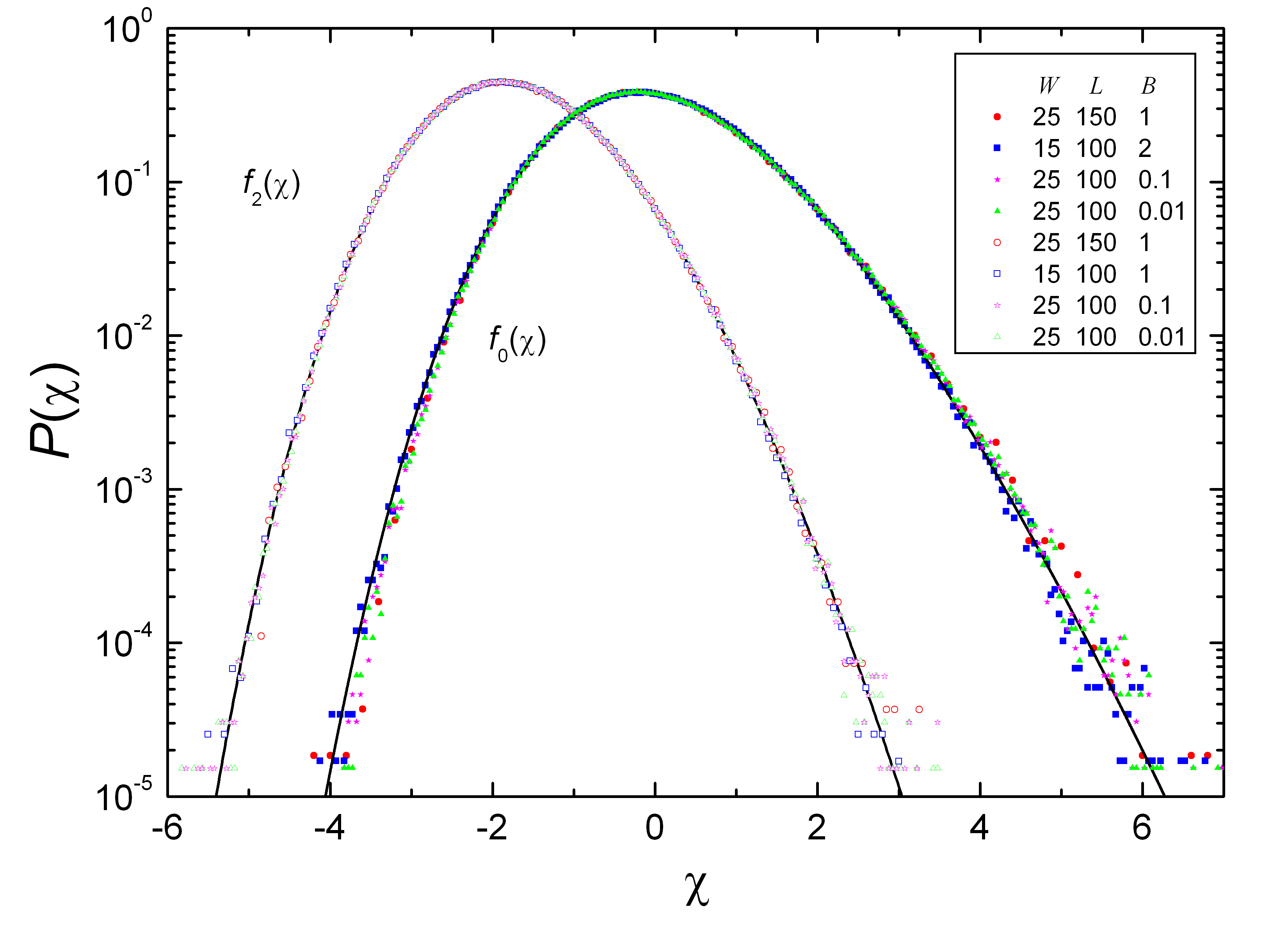
Figure 7: Histogram of $\ln g$ for the Anderson model with an applied magnetic field for narrow (empty symbols) and wide (solid symbols) leads for the values of the disorder, system size and magnetic field given in the figure. The continuous lines correspond to $f_{2}(\chi_{2})$ and $f_{0}(\chi_{0})$.

The results indicate that the magnetic field does not change the percolative nature of the conduction in the strongly localized regime.

The value of $\beta$ in Eqs. (16) and (19) changes very little with the applied field, less than our uncertainty in the measurements.

We have also checked that the application of a magnetic field in the NSS model with narrow leads produces negative magnetoresistance, but does not change the distribution function. To be quantitative, we have plotted in Fig. 8 the skewness as a function of $L^{-2/3}$ for several values of the magnetic field, detailed in the legend of the figure. The horizontal line corresponds to the skewness of the distribution $f_{2}$ and the lower curve to the situation in the absence of a magnetic field. The skewness clearly tends to the TW value, as the system size tends to infinity, for all cases considered. We note that in the presence of a field the convergence is faster than in its absence. It is also interesting to note the dependence of the slopes in Fig. 8 with magnetic field. They increase with the field, while the value in the absence of a field is larger than in the presence of it.

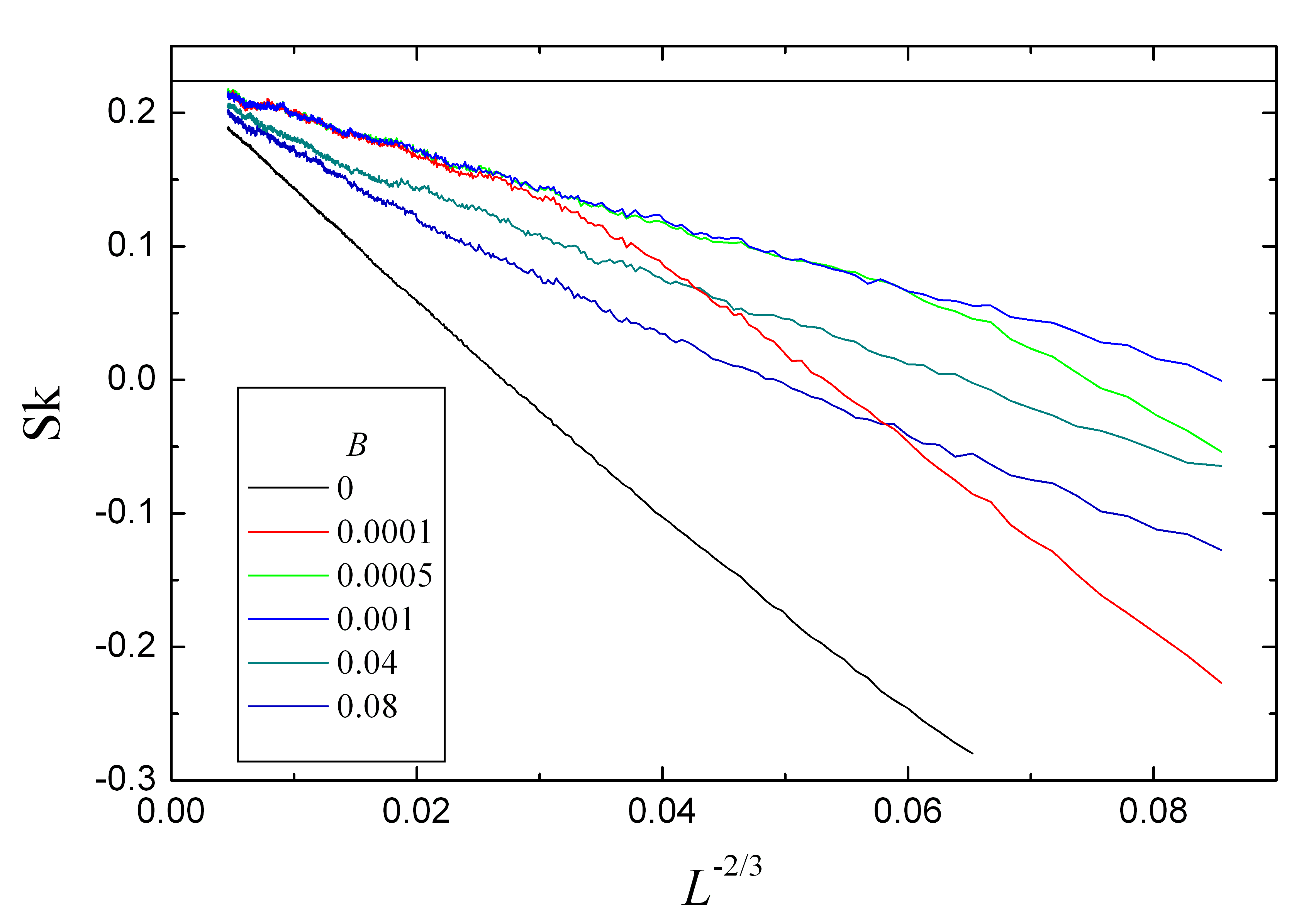
Figure 8: Skewness as a function of $L^{-2/3}$ for several values of the magnetic field in the NSS model with narrow leads. The horizontal line corresponds to the TW value.

7 Discussion and conclusions

Present results confirm our previous belief that, in the strongly localized regime, directed path models are in the same universality class as the Anderson model SP06 ; NS85 ; MK92 . While the NSS model pretended to maximize interference effects, Johansson’s model only considers the most important path. The agreement between both models indicates that it is percolation and not interference the dominant effect in this regime. We expect that the main effect of interference between different paths is a renormalization of the disorder energies. This information may be relevant to deal with interacting systems, since for many properties FSP models are a good approximation to the Anderson model and they can be extended to many-particle systems, whose direct simulation may be feasible for relatively large systems.

The distribution functions of the conductance in the FPS approximation and the Anderson model appear in many other problems. Our results are fully consistent with the strong version of the SPS SM01 if we take into account that boundary conditions (leads) are not irrelevant variables in the renormalization group sense, and may change the universality class. We have checked that the skewness and the kurtosis obtained numerically for narrow leads tend to the theoretical predictions. We finally showed that the conductance distribution does not change when we apply a magnetic field.

The situation in 3D systems is more complex, since analytical approaches valid for 2D systems do not apply. There are no hints of distribution functions for any similar type of problem. Nevertheless, the quality of the fit in 2D systems suggests that numerical simulations will provide useful information.

References

- (1) D. J. Thouless, Phys. Rep. 13, 93 (1974); Phys. Rev. Lett. 39, 1167 (1977).
- (2) E. Abrahams, P.W. Anderson, D.C. Licciardello and T.V. Ramakrishnan, Phys. Rev. Lett. 42, 673 (1979).
- (3) B. Shapiro, Phil. Mag. B 56, 1031 (1987); A. Cohen, Y. Roth and B. Shapiro, Phys. Rev. B 38, 12125 (1988).
- (4) P. J. Roberts, J. Phys.: Condens. Matter 4, 7795 (1992).
- (5) P. W. Anderson, D. J. Thouless, E. Abrahams, D. S. Fisher, Phys. Rev. B 22, 3519 (1980).
- (6) K. Chase and A. MacKinnon, J. Phys. C 20, 6189 (1987).
- (7) B. Kramer, A. Kawabata and M. Schreiber, Phil. Mag. B 65, 595 (1992).
- (8) B. Kramer and A. MacKinnon, Rep. Prog. Phys. 56, 1469 (1993).
- (9) P. Markoš, Phys. Rev. B 65, 104207 (2002).
- (10) P. Markoš, K. A. Muttalib, P. Wölfle and J. R. Klauder, Europhys. Letters 68, 867 (2004); P. Markoš, Acta Physica Slovaca 56, 561 (2006).
- (11) K. A. Muttalib, P. Markoš and P. Wölfle, Phys. Rev. B 72, 125317 (2005).
- (12) J. Prior, A. M. Somoza and M. Ortuño, Phys. Stat. Solidi (b) 243, 395 (2006).
- (13) J. Prior, A. M. Somoza and M. Ortuño, Phys. Rev. B 72, 024206 (2005).
- (14) A. M. Somoza, J. Prior and M. Ortuño, Phys. Rev. B 73, 184201 (2006).
- (15) J. M. Kim, M. A. Moore and A. J. Bray, Phys. Rev. A 44, 2345 (1991).
- (16) V. L. Nguyen, B. Z. Spivak and B. I. Shklovskii, Pis’ma Zh. Eksp. Teor. Fiz. 41, 35 (1985) [JETP Lett. 41, 42 (1985)]; Zh. Eksp. Teor. Fiz. 89, 11 (1985) [Sov. Phys.–JETP 62, 1021 (1985)].
- (17) E. Medina and M. Kardar, Phys. Rev. B 46, 9984 (1992); E. Medina, M. Kardar, Y. Shapir and X. R. Wang, Phys. Rev. Lett. 62, 941 (1989).
- (18) C.A. Tracy and H. Widom, Commun. Math. Phys. 159, 151 (1994); 177, 727 (1996).
- (19) J. Baik, P. A. Deift and K. Johansson, J. Amer. Math. soc. 12, 1119 (1999).
- (20) S. N. Majumdar, AxXiv: cond-mat/0701193v1.
- (21) K. Johansson, Commun. Math. Phys. 209, 437 (2000).
- (22) M. Prähofer and H. Spohn, Phys. Rev. Lett. 84, 4882 (2000); J. Baik and E. M. Rains, J. Stat. Phys. 100, 523 (2000).
- (23) M. Kardar, G. Parisi and Y. C. Zhang, Phys. Rev. Lett. 56, 889 (1986).
- (24) A. M. Somoza, M. Ortuño, and J. Prior Phys. Rev. Lett. 99, 116602 (2007).
- (25) A. MacKinnon, Z. Phys. B 59, 385 (1985).
- (26) J.A. Verges, Comput. Phys. Commun. 118, 71 (1999).
- (27) L. Schweitzer, B. Kramer and A. MacKinnon, J. Phys. C 17, 4111 (1984).
- (28) Y.C. Zhang, Europhys. Lett. 7, 113 (1989).
- (29) K. Slevin, P. Markos and T. Ohtsuki, Phys. Rev. Lett. 86, 3594 (2001).