The effect of mechanical stirring on horizontal convection

Abstract

The theoretical analysis of the energetics of mechanically-stirred horizontal convection for a Boussinesq fluid yields the formula:

$$G(APE)=\gamma_{mixing}G(KE)+(1+\gamma_{mixing})W_{r,laminar}$$

where $G(APE)$ and $G(KE)$ are the work rate done by the buoyancy and mechanical forcing respectively, $\gamma_{mixing}$ is the mixing efficiency, and $W_{r,laminar}$ is the background rate of increase in gravitational potential energy due to molecular diffusion. The formula shows that mechanical stirring can easily induce a very strong buoyancy-driven overturning cell (meaning a large $G(APE)$) even for a relatively low mixing efficiency, whereas this is only possible in absence of mechanical stirring if $\gamma_{mixing}\gg 1$. Moreover, the buoyancy-driven overturning becomes mechanically controlled when $\gamma_{mixing}G(KE)\gg(1+\gamma_{mixing})W_{r,laminar}$. This result explains why the buoyancy-driven overturning cell in the laboratory experiments by Whitehead et al. (2008) is amplified by the lateral motions of a stirring rod. The formula implies that the thermodynamic efficiency of the ocean heat engine, far from being negligibly small as is commonly claimed, might in fact be as large as can be thanks to the stirring done by the wind and tides. These ideas are further illustrated by means of idealised numerical experiments. A non-Boussinesq extension of the above formula is also given.

1 Introduction

A fundamental objective of ocean circulation theory is to characterise and quantify the relative importance of the mechanical and thermodynamical forcing in driving and stirring the oceans. Although the oceans are highly nonlinear a system, ocean circulation theory nevertheless historically evolved under the assumption that separate theories for the wind-driven and buoyancy-driven circulation could be developed, as it the two kind of circulation could be regarded as somehow decoupled. From a thermodynamic viewpoint, this is somehow justified from the fact that mechanical forcing, unlike the buoyancy forcing, does not modify the fluid parcels’ buoyancy, suggesting that distinct effects should be observable. In the thermodynamic engineering literature, mechanical forcing is commonly regarded as “shaft” work, which alters the energy of the fluid without altering its total entropy. In oceanographic textbooks, wind-driven circulation theories usually occupy a more prominent place that buoyancy-driven circulation theories. Indeed, it turns out to be relatively easy to link the near surface transport (Ekman theory) or the vertically-integrated transport (Sverdrup theory) to the wind stress or its spatial derivatives in a quantitative relatively accurate way. Theories for the buoyancy-driven circulation, on the other hand, are often more qualitative, and at best offer only tentative scaling arguments to relate the strength of the large-scale overturning cell taking place in the meridional/vertical plane, e.g. (Colin de Verdière1993). From a physical viewpoint, the two main salient ingredients of the buoyancy-driven circulation have been traditionally associated with high-latitude cooling, envisioned as the destabilising mechanism setting up the meridional overturning circulation into motion, and turbulent diapycnal mixing, envisioned as the process required to carry heat from the surface at the depths cooled by deep water formation, thus precluding the oceans to fill up with dense and salty waters.

Physically, however, the buoyancy-driven circulation can only be regarded as independent of the mechanical forcing if one can establish that the stirring required to maintain turbulent diapycnal mixing is predominantly sustained by the work rate done by the surface buoyancy fluxes $G(APE)$ (i.e., the rate of available potential energy production, see Lorenz (1955)). A crucial question, therefore, is how large is $G(APE)$? In their observational analysis of ocean energetics, Oort et al. (1994) found $G(APE)=1.2\pm 0.7{\rm TW}$, and concluded that the buoyancy forcing was as important as the wind in forcing and stirring the oceans. This result, however, was challenged by Munk et al. (1998) (MW98 thereafter), who contended that the so-called Sandström (1908)’s theorem forbids $G(APE)$ to be significant, and hence that turbulent diapycnal mixing must be primarily be sustained by the work rate done by the mechanical forcing due to the wind and tides, leading to the idea that the buoyancy-driven circulation is actually mechanically-driven. MW98 furthermore sought to quantify the magnitude of the mechanical sources of stirring required to sustain diapycnal mixing in the oceans. Their main result is the following formula:

$$G(KE)=\frac{W_{r,forcing}}{\gamma_{mixing}},$$ (1)

where $G(KE)$ is the work rate done by the mechanical sources of stirring, $W_{r,forcing}$ is the rate at which the background gravitational potential energy $GPE_{r}$ decreases as the result of high-latitude cooling, and $\gamma_{mixing}$ is the so-called mixing efficiency, e.g., Osborn (1980). MW98 estimated $W_{r,forcing}\approx 0.4\,{\rm TW}$ from assuming the deep water formation rate to be known, and used the canonical value $\gamma_{mixing}=0.2$ for the mixing efficiency to conclude that $G(KE)=O(2\,{\rm TW})$ was required to sustain the observed rate of turbulent diapycnal mixing and its associated poleward heat transport of about $2\,{\rm PW}$. Since the wind forcing provides no more than about $1\,{\rm TW}$, this result suggests an apparent shortfall of about $1\,{\rm TW}$ of mechanical stirring that MW98 argued must only come from the work rate done by the tides, spawning much research over the past decade on the issue of tidal mixing.

MW98’s study prompted much debate over the past decade about the relative importance of the surface buoyancy forcing, and about whether Sandstrom’s theorem really implied for $G(APE)$ to be negligible. Recently, Tailleux (2009) revisited a number of misconceptions about the nature of energy conversions in turbulent stratified fluids by extending the available potential energy framework of Winters et al. (1995) to the fully compressible Navier-Stokes equations (CNSE thereafter). One of the main result was to demonstrate from first principles that:

$$G(APE)\approx W_{r,forcing},$$ (2)

which physically states that the production rate of $APE$ is approximately equal to the rate at which $GPE_{r}$ decreases as the result of high-latitude cooling. This result is extremely important, because it rigourously proves that it is inconsistent to assume $W_{r,forcing}$ to be large while simultaneously assuming $G(APE)$ to be negligible, as done in MW98. As a result, rather than establishing that the work rate done by surface buoyancy forcing is small, MW98’s study actually establishes precisely the contrary, since their estimate $W_{r,forcing}\approx 0.4\,{\rm TW}$ implies $G(APE)\approx 0.4\,{\rm TW}$, which turns out to be very close to Oort et al. (1994)’s lower bound for $G(APE)$. Moreover, Tailleux (2009) was able to show that a generalisation of MW98’s Eq. (1) for a non-Boussinesq fluid can be rigourously derived from first principles by combining the mechanical energy budget for $APE$ and $GPE_{r}$ separately, the final result taking the form:

$$G(KE)=\frac{1+(1-\xi)\gamma_{mixing}}{\xi\gamma_{mixing}}G(APE)$$

$$=\frac{1-\xi R_{f}}{\xi R_{f}}G(APE),$$ (3)

where $\xi$ is a non-Boussinesq nonlinearity parameter which is such that $-\infty<\xi\leq 1$ for water and seawater, $\gamma_{mixing}$ is the mixing efficiency, and $R_{f}=\gamma_{mixing}/(1+\gamma_{mixing})$ is the so-called flux Richardson number, e.g., Osborn (1980). MW98’s Eq. (1) is recovered in the limiting case $\xi=1$ describing a Boussinesq fluid with a linear equation of state, by using the above result that $G(APE)\approx W_{r,forcing}$.

The fact that the generalisation of MW98’s result can be written as a formula linking $G(KE)$ and $G(APE)$ rather than $G(KE)$ and $W_{r,forcing}$ raises the question of whether it is really appropriate to interpret Eq. (3) (and hence Eq. (1)) as a constraint on the amount of $G(KE)$ required to sustain diapycnal mixing in the oceans, as suggested by MW98. Indeed, it seems that such an interpretation implicitly assumes that both $G(APE)$ and $\gamma_{mixing}$ can be regarded as fixed in some sense, but whether this is the correct way to interpret Eq. (3) is unclear, given that the latter can be rewritten in the two following ways:

$$G(APE)=\frac{\xi\gamma_{mixing}}{1+(1-\xi)\gamma_{mixing}}G(KE),$$ (4)

or as:

$$\xi R_{f}=\frac{G(APE)}{G(KE)+G(APE)},$$ (5)

i.e., under the form of a constraint either on $G(APE)$ or on $\xi R_{f}$. Note that from observations, plausible numbers for the wind and buoyancy forcing are $G(KE)\approx 1\,{\rm TW}$ and $G(APE)\approx 0.5\,{\rm TW}$, which, if inserted into Eq. (5) yields:

$$\xi R_{f}\approx\frac{0.5}{1.5}=0.3333.$$

Another way to pose the problem initially formulated by MW98 would be to ask the question of whether the above value for $\xi R_{f}$ can be ruled out from what we know about mixing efficiency (and the role played by the nonlinearity of the equation of state, but we know less about the latter). Although the value $\gamma_{mixing}\approx R_{f}\approx 0.2$ is often assumed, it is important to realize that such value mostly pertains to mechanically-driven turbulent mixing, as occurs in relation with shear flow instability for instance. Indeed, mixing efficiency values as high as $R_{f}=0.5$ ($\gamma_{mixing}=1$) have been reported by Dalziel et al. (2008) for buoyancy-driven mixing associated with Rayleigh-Taylor instability. Since $G(APE)$ is comparable to $G(KE)$, values of $\gamma_{mixing}$ intermediate between those for mechanically- and buoyancy-driven mixing should be expected.

In trying to figure out the exact physical meaning of Eq. (3), it is important to discuss the nature and structure of $G(KE)$ and $G(APE)$ in more details. Thus, the work rate done by the wind stress is given by:

$$G(KE)=\int_{S}{\bf\tau}\cdot{\bf u}_{s}dS$$ (6)

where $\tau$ is the wind stress at the ocean surface, and ${\bf u}_{s}$ is the ocean surface velocity. The important point about $G(KE)$ is that it is a correlation between the external forcing (the wind stress) and a parameter depending upon the particular state of the system (the surface velocity). In other words, it is essential to realize that $G(KE)$ cannot be determined from the knowledge of the external forcing alone. This is important, because Eq. (6) expresses the possibility for the wind-driven circulation to be controlled by the buoyancy forcing, to the extent that the latter is able to influence the surface velocity. In order to gain insight into the potential importance of the buoyancy control of the wind-driven circulation, it would be interesting to compute $G(KE)$ for a purely wind forced homogeneous ocean model. Doing so, however, is beyond the scope of this paper. For the present purposes, we shall assume that $G(KE)$ is primarily determined by the wind forcing, and that buoyancy forcing only alters it as a second order effect, which seems plausible on the basis that the near surface circulation in the oceans is usually thought to be the signature of the wind forcing rather than the buoyancy forcing.

With regard to the work rate done by surface buoyancy fluxes, it was shown by Tailleux (2009) to be given by the following expression:

$$G(APE)=\int_{S}\frac{T-T_{r}}{T}Q_{surf}dS,$$ (7)

in the case of a compressible thermally-stratified fluid forced by surface heat fluxes, where $T$ is the surface temperature of the fluid parcels, and $T_{r}$ the temperature the surface parcels would have if displaced adiabatically to their level in Lorenz (1955)’s reference state, while $Q_{surf}$ is the diabatic rate of heating cooling/heating due to the surface heat fluxes. Useful approximations for $G(APE)$ can be obtained by expanding $T$ as a Taylor series expansion around the surface pressure $P_{a}$, i.e., $T\approx T_{r}+\Gamma_{r}(P_{a}-P_{r})+O((P_{a}-P_{r})^{2})$, where $\Gamma_{r}=\alpha_{r}T_{r}/(\rho_{r}C_{pr})$ is the adiabatic lapse rate, leading to:

$$G(APE)\approx-\int_{S}\frac{\alpha_{r}(P_{r}-P_{a})}{\rho_{r}C_{pr}}Q_{surf}dS$$

$$\approx\int_{S}\frac{\alpha_{r}gz_{r}}{C_{pr}}Q_{surf}dS,$$ (8)

by using the approximation $P_{r}-P_{a}\approx-\rho_{0}gz_{r}$, the latter expression being actually the Boussinesq approximation of $G(APE)$ derived by Winters et al. (1995) provided that one regards the thermal expansion $\alpha_{r}$ and specific heat capacity $C_{pr}$ as constant (the suffix $r$ means that the variables have to be estimated in Lorenz (1955)’s reference state). As for $G(KE)$, $G(APE)$ also takes the form of a correlation between the external forcing (the heating/cooling rate at the surface) and a parameter depending on the particular state of the system, namely $(T-T_{r})/T\approx\alpha_{r}(P_{a}-P_{r})/(\rho_{r}C_{pr})\approx\alpha_{r}gz_{r}/C_{pr}$. Eqs. (7) and (8) make it possible, therefore, for the buoyancy-driven circulation to be mechanically-controlled. Physically, this is expected, because mechanical forcing is widely agreed to increase diapycnal mixing, which should produce a deeper thermocline, thereby allowing dense plumes to penetrate deeper, thus increasing $G(APE)$ and hence the buoyancy-driven circulation. Interestingly, this appears consistent with the laboratory experiments by Whitehead et al. (2008) which provide evidence that the lateral motion of a stirring rod can greatly enhance the strength of horizontal convection (see Hughes et al. (2008) for a review on this topic). This paper examines the possibility of interpreting this result as the consequence that $G(APE)$, and hence the buoyancy-driven circulation, is increased by the work rate done by the stirring rod. To that end, Section 2 seeks to extend Eq. (3) to also describe the purely buoyancy-driven case for which it is not valid. The physical meaning of the extended formula is then explored by means of idealised numerical experiments in Section 3. Finally, section 4 presents a discussion of the results.

2 Theoretical results about the effects of mechanical stirring on the work rate done by surface buoyancy fluxes

2.1 Summary of Tailleux (2009)’s theory

Our starting point is the theoretical description of the energetics of mechanically and thermodynamically forced turbulent stratified fluids recently derived by Tailleux (2009) pertaining to a thermally-stratified fluid governed by the fully compressible Navier-Stokes equations (NCSE thereafter), which builds upon the available potential energy framework previously introduced by Winters et al. (1995) for a Boussinesq fluid with a linear equation of state. In Tailleux (2009)’s description, the energetics is described at leading order by means of the following five evolution equations:

$$\frac{d(KE)}{dt}=-C(KE,APE)+G(KE)-D(KE),$$ (9)

$$\frac{d(APE)}{dt}=C(KE,APE)+G(APE)-D(APE),$$ (10)

$$\frac{d(GPE_{r})}{dt}=W_{r,turbulent}+W_{r,laminar}-W_{r,forcing},$$ (11)

$$\frac{d(IE_{0})}{dt}=(1-\Upsilon_{0})\dot{Q}_{net}+D(APE)+D(KE)-G(APE),$$ (12)

$$\frac{d(IE_{exergy})}{dt}=\Upsilon_{0}\dot{Q}_{net}-W_{r,turbulent}-W_{laminar},$$ (13)

where $KE$ is the volume-integrated kinetic energy, $APE$ is Lorenz (1955)’s volume-integrated available potential energy, $GPE_{r}$ is the volume-integrated gravitational potential energy of Lorenz (1955)’s reference-state, $IE_{0}$ is the volume-integrated of a subcomponent of internal energy $(IE)$ that we call the dead part of $IE$, $IE_{exergy}$ is the volume-integrated of another subcomponent of $IE$ called the exergy. Physically, variations in $IE_{0}$ are associated with variations in the equivalent thermodynamic equilibrium temperature $T_{0}(t)$ of the system, whereas variations in $IE_{exergy}$ reflect variations in the reference temperature profile $T_{r}(z,t)$. The other important conversion terms are $C(KE,APE)$, the so-called buoyancy flux that represents the reversible conversion between $KE$ and $APE$; $G(APE)$, the production rate of $APE$ that physically represents a conversion between $IE_{0}$ and $APE$; $W_{r,laminar}$ and $W_{r,turbulent}$ represent the laminar and turbulent rate of exchange between $IE_{exergy}$ and $GPE_{r}$ due to molecular diffusion; $D(KE)$ is the dissipation rate of $KE$ into internal energy $IE_{0}$ by molecular viscous processes; $D(APE)$ is the dissipation rate of $APE$ into internal energy $IE_{0}$ by molecular diffusive processes. The parameter $\Upsilon_{0}\ll 1$ plays the role of a thermodynamic efficiency that is very small for a nearly incompressible fluid, and which controls how much of the net surface heating rate $\dot{Q}_{net}$ splits between $IE_{exergy}$ and $IE_{0}$.

As previously shown by Winters et al. (1995), a number of conversion terms appear to be strongly correlated to each other. This is the case for $D(APE)$ and $W_{r,turbulent}$, owing to both terms: 1) being controlled by molecular diffusion; 2) being controlled by the spectral distribution of the $APE$ density, see Holliday et al. (1981) and Roullet et al. (2009) for a discussion of the latter concept. For a compressible thermally-stratified fluid, Tailleux (2009) showed that this correlation between $D(APE)$ and $W_{r,turbulent}$ can be written under the general form:

$$W_{r,turbulent}=\xi D(APE)$$ (14)

where $\xi$ is a parameter that measures the importance of the nonlinearity of the equation of state, such that $\xi=1$ for a Boussinesq fluid with a linear equation of state, but $-\infty<\xi\leq 1$ for water or seawater. The second type of conversion terms that are correlated to each other are $G(APE)$ and $W_{r,forcing}$ owing to both terms being controlled by the surface buoyancy forcing. Tailleux (2009) shows that to a good approximation, one usually has:

$$G(APE)\approx W_{r,forcing}.$$ (15)

For the sake of brevity, the reader is referred to Tailleux (2009) for the details about the explicit forms of all the terms entering the above energy equations, as they are unimportant for the arguments developed in this paper. Fig. (1) schematically illustrates the energetics of a mechanically and thermodynamically forced stratified fluids associated with the above equations. For all practical purposes, $G(APE)$ and $G(KE)$ represent the work rate done by the buoyancy and mechanical forcing respectively, whereas $D(APE)$ and $D(KE)$ represent the two terms dissipating the “available” mechanical energy $ME=APE+KE$.

2.2 A general theory for $G(APE)$

A fundamental question posed by this paper is what controls the magnitude of the buoyancy-driven circulation, that is, the circulation drawing its energy from $G(APE)$, with and without mechanical stirring acting on the fluid. In order to answer this question, we first need to introduce a couple of parameters that are traditionally used to measure the efficiency of turbulent mixing, the so-called mixing efficiency $\gamma_{mixing}$ and the flux Richardson number $R_{f}$, which are defined here as follows:

$$\gamma_{mixing}=\frac{D(APE)}{D(KE)},$$ (16)

$$R_{f}=\frac{\gamma_{mixing}}{1+\gamma_{mixing}}=\frac{D(APE)}{D(APE)+D(KE)}.$$ (17)

The physical rationale for such definitions, as well as their connection to other existing definitions, was discussed in details in Tailleux (2009) to which the reader is referred to for details. From a practical viewpoint, the differences in existing definitions is unimportant, as least in the context of a Boussinesq fluid, as then all definitions are then numerically equivalent, even if based on different physical assumptions. In particular, the present definitions allow to recover MW98’s Eq. (1), as discussed below. To distinguish them from existing definitions, Tailleux (2009) refer to the above $\gamma_{mixing}$ and $R_{f}$ as the ”dissipative” mixing efficiency and flux Richardson number respectively.

In a second step, the mechanical energy balance is constructed by summing the steady-state version of the $KE$ and $APE$ equations, which yields:

$$G(APE)+G(KE)=D(APE)+D(KE).$$ (18)

Now, by combining this equation with the definition of the flux Richardson number (i.e., Eq. (17), one may write:

$$D(APE)=R_{f}[G(APE)+G(KE)].$$ (19)

Next, we turn to the steady-state $GPE_{r}$ balance, viz.,

$$W_{r,turbulent}+W_{r,laminar}=W_{r,forcing}.$$ (20)

As mentioned above, one has to a very good approximation the following equality $W_{r,forcing}\approx G(APE)$. For mathematical rigour, we introduce a parameter $\xi_{2}\approx 1$ making exact the equality $W_{r,forcing}=\xi_{2}G(APE)$. Using the definition of $\xi$ above, the $GPE_{r}$ budget provides the following relationship:

$$\xi D(APE)+W_{r,laminar}=\xi_{2}G(APE),$$ (21)

which after some algebra eventually yields:

$$G(APE)=\frac{\xi R_{f}}{\xi_{2}-\xi R_{f}}G(KE)+\frac{W_{r,laminar}}{\xi_{2}-\xi R_{f}}.$$ (22)

Eq. (22) is one of the most important result of this paper, as it represents one way to demonstrate the interconnection of the work rate done by the wind and buoyancy forcing in general. A useful limit is the case of the widely used Boussinesq model for which $\xi=\xi_{2}=1$, in which case Eq. (22) simplifies to:

$$G(APE)=\frac{R_{f}}{1-R_{f}}G(KE)+\frac{W_{r,laminar}}{1-R_{f}}$$

$$=\gamma_{mixing}G(KE)+(1+\gamma_{mixing})W_{r,laminar}.$$ (23)

Eq. (22) shows that in absence of mechanical forcing, the work rate done by the surface buoyancy fluxes is given by:

$$G(APE)=\frac{W_{r,laminar}}{\xi_{2}-\xi R_{f}}$$ (24)

or, for a Boussinesq fluid:

$$G(APE)=\frac{W_{r,laminar}}{1-R_{f}}=(1+\gamma_{mixing})W_{r,laminar}.$$ (25)

The latter two results are interesting, because they show that although $W_{r,laminar}$ is small by construction, it does not forbid in principle $G(APE)$ to be large provided that $\xi_{2}-\xi R_{f}$ or $1-R_{f}$ can become small enough. The problem, however, is that the latter conditions require $R_{f}$ to be close to unity for a Boussinesq fluid, or equivalently $\gamma_{mixing}\gg 1$, which is much larger than the widely used canonical value $\gamma_{mixing}\approx 0.2$. On the other hand, we are not aware of any published value for $\gamma_{mixing}$ pertaining to horizontal convection, so that sufficient empirical evidence to be really conclusive. The idealised numerical experiments presented below seeks to get insight into this issue.

Perhaps the most important feature of Eq. (22) is to reveal that even a small amount of mechanical forcing is sufficient to radically alter the nature of horizontal convection, as it suggests that the latter becomes mechanically controlled when $G(KE)$ is such that $\xi R_{f}G(KE)\gg W_{r,laminar}$, which is possible even for relatively low values of $\gamma_{mixing}$ — a very important point. This theoretical result suggests therefore that $G(APE)$ can be dramatically enhanced by the presence of mechanical stirring, provided that the latter provides positive work to the system (i.e., such that $G(KE)>0$). Negative work, on the other hand, should reduce the strength of the buoyancy-driven circulation. The numerical examples studied next seek to illustrate these different ideas.

Figure 1: Schematic diagram of the energy conversions taking place in a mechanically and thermodynamically forced turbulent thermally-stratified fluid corresponding to Eqs. (9-13) previously derived by Tailleux (2009).

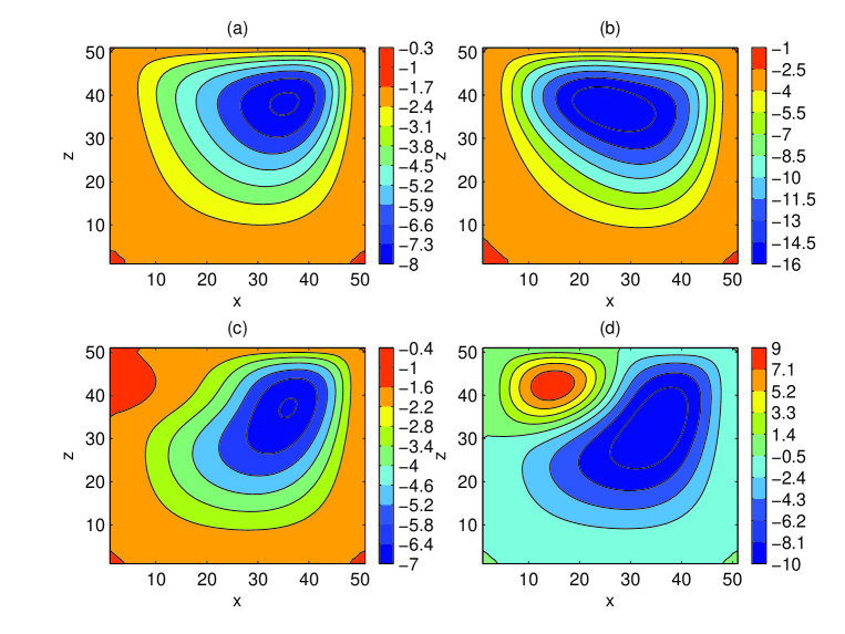
Figure 2: Streamfunction for the different experiments: (a) No mechanical forcing; (b) Clockwise mechanical forcing; (c) Weak anti-clockwise mechanical forcing; (d) Strong anti-clockwise mechanical forcing.

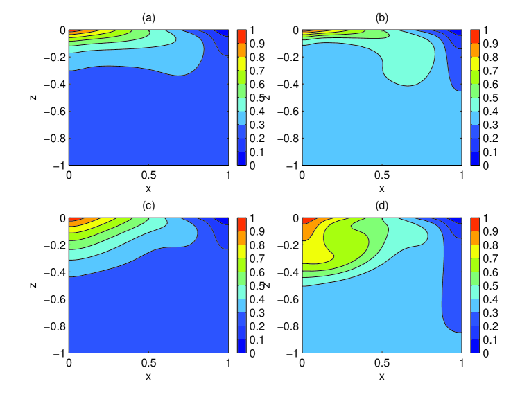
Figure 3: Temperature field for the different experiments: (a) No mechanical forcing; (b) Clockwise mechanical forcing; (c) Weak anti-clockwise mechanical forcing; (d) Strong anti-clockwise mechanical forcing.

3 Numerical experiments

The physical implications of the formula given by Eqs. (22) and (23) are explored in the following by means of numerical experiments aiming at illustrating the main effects mechanical stirring can have on buoyancy-driven circulations.

3.1 Model description

To that end, the idealised problem of horizontal convection previously considered by Paparella et al. (2002) is investigated here, the novelty being the addition of mechanical stirring to the problem modelled here as a forcing term in the vorticity equation. The numerical implementation of such a model is that previously described by Marchal (2007). The equations solved by the numerical model are the Boussinesq equations for a fluid with a linear equation of state:

$$\frac{\partial\omega}{\partial t}=J(\Psi,\omega)-g\alpha\frac{\partial T}{\partial x}+\nu\nabla^{2}\omega+F(x,z,t)$$ (26)

$$\frac{\partial T}{\partial t}=J(\Psi,T)+\kappa\nabla^{2}T,$$ (27)

where $\omega=\nabla^{2}\Psi$ is the vorticity, $T$ is the temperature, $J(a,b)=\partial a/\partial x\partial b/\partial z-\partial a/\partial z\partial b/\partial x$ is the Jacobian operator, $g$ is the acceleration due to gravity, $\alpha$ is the thermal expansion coefficient assumed to be constant, $\nu$ is the kinematic viscosity, $\kappa$ is the thermal diffusivity, and $F$ is a term aimed at modelling the effect of mechanical stirring.

Following Marchal (2007), the above system is made dimensionless as follows: $t=(L^{2}/\kappa)t^{\ast}$, $(x,z)=L(x_{\ast},z_{\ast})$, $\omega=(\kappa/L^{2})\omega_{\ast}$, $T=\Delta TT_{\ast}$, and $\Psi=\kappa\Psi_{\ast}$, where the starred quantities are the dimensionless ones. The dimensionless forms of the above equations become, after dropping the start for clarity:

$$\frac{\partial\omega}{\partial t}=J(\Psi,\omega)+P_{r}\left(-R_{a}\frac{\partial T}{\partial x}+\nabla^{2}\omega\right)+F^{\ast},$$ (28)

$$\frac{\partial T}{\partial t}=J(\Psi,T)+\nabla^{2}T,$$ (29)

where $R_{a}=g\alpha\Delta T^{3}/(\nu\kappa)$ is the Rayleigh number, and $P_{r}=\nu/\kappa$ is the Prandtl number. In the numerical experiments described here, we used $P_{r}=10$ and $R_{a}=10^{5}$. For comparison, note that typical oceanic values are $R_{a}=O(10^{20})$, e.g., Paparella et al. (2002).

As in Paparella et al. (2002), the fluid is forced by a surface temperature boundary condition varying linearly in $x$. The numerical resolution used for the experiments is $51\times 51$ in a 2-D square geometry. At equilibrium, the forcing term in the vorticity equation is associated with the work rate:

$$G(KE)=\int\int_{V}F\Psi\,dxdz$$ (30)

which can be in principle either positive or negative.

3.2 Experiments

Four idealised experiments were considered:

1. Purely buoyancy-driven (i.e., no mechanical forcing);

2. Clockwise Mechanical forcing;

3. Weak anti-clockwise mechanical forcing;

4. Strong anti-clockwise mechanical forcing.

The purely buoyancy-driven case is associated with a clock-wise thermally-direct circulation, and represents the “control” reference simulation to be compared with the mechanically-stirred ones. The purpose of Experiment (ii) is to gain insight into the case for which the mechanical stirring tends to re-enforce the existing thermally-direct clockwise circulation, implying $G(KE)>0$. From Eq. (23), the expectation is that the overturning circulation should increase both as the result of increased $G(APE)$, as well as from the direct effect of the mechanical forcing acting as a source of clockwise vorticity. In such a case, therefore, $KE$, $APE$, $\Psi$, $D(APE)$ and $G(APE)$ all should increase.

In experiments (iii) and (iv), however, the anti-clockwise forcing works against the existing buoyancy-driven circulation. If too weak, as designed to be the case for (iii), the mechanical forcing is unable to reverse the sense of the existing thermally-direct circulation anywhere, resulting in $G(KE)<0$. According to Eq. (23), a decrease in all quantities $KE$, $APE$, $\Psi$, $D(APE)$, and $G(APE)$ is expected in that case. If the clockwise forcing is strong enough, however, it can locally generate a anti-clockwise circulation associated with $G(KE)>0$, making it possible in that case for all above quantities to be increased.

3.3 Results

	G(KE)	G(APE)	D(APE)	$\gamma_{mixing}$
(a)	0	5.98	4.12	1.78
(b)	7.54	10.1	9.52	1.04
(c)	-0.77	4.72	2.58	1.49
(d)	9.83	8.50	7.18	0.60

Table 1: Values of the work rate done by the mechanical forcing $G(KE)$, rate of $APE$ production $G(APE)$, diffusive $APE$ dissipation rate $D(APE)$, and mixing efficiency $\gamma_{mixing}$ for (a) No mechanical forcing; (b) Clockwise mechanical forcing; (c) Weak anti-clockwise mechanical forcing; (d) Strong anti-clockwise mechanical forcing.

	KE	APE	$\Psi_{max}$	$H_{max}$
(a)	0.13	4.04	7.2	3.15
(b)	0.64	6.25	15.5	5.09
(c)	0.09	5.49	6.08	2.19
(d)	0.51	11.1	9.67	2.75

Table 2: Values of the volume-integrated kinetic energy $KE$, volume-integral available potential energy $APE$, maximum value of the thermally-direct overturning streamfunction, and maximum value of the heat transport for: (a) no mechanical forcing; (b) Clockwise mechanical forcing; (c) Weak anti-clockwise mechanical forcing; (d) Strong anti-clockwise mechanical forcing.

The results are illustrated by the figs. (2) and (3), which show the streamfunction and temperature distributions for the 4 different experiments considered. In addition, Tables 1 and 2 summarise how several important quantities vary as a function of the mechanical forcing imposed. As expected, all the plots for $\Psi$ show evidence of a well-marked thermally-direct cell in all cases. Fig. (2) (b) shows that the strength of the overturning cell is greatly enhanced by the addition of clockwise mechanical forcing. This can be explained by the observed increase in $G(APE)$ (Table 1), as well as by the direct effect of the mechanical forcing as a source of clockwise vorticity. Fig. 3 (b) shows that the increase in $G(APE)$ is associated with the dense plumes penetrating deeper in that case. Fig. (2) (c) shows that a weak anti-clockwise mechanical forcing decreases the buoyancy-driven circulation, which is expected from the theory when $G(KE)<0$ as is the case here (Table 1). The weakening of the circulation results from the decrease in $G(APE)$, despite an apparent increase in the thermocline depth (Fig. 3) which one would normally associate with an increase in $G(APE)$. As shown in Table 2, this occurs because of a reduction in the strength of the surface heat flux, which results in a decrease in the maximum heat transport $H_{max}$. Fig. (2) (d) shows that the anti-clockwise mechanical forcing is strong enough to generate a thermally-indirect circulation, resulting in $G(KE)>0$, which increases the overturning strength. In that case, there is no ambiguity that the increase in the latter is entirely explained by the increase in $G(APE)$, given that the mechanical forcing acts as a source of anti-clockwise vorticity, which can only tend to weaken the buoyancy-driven thermally-direct cell.

In the literature, there is a tendency to regard the mixing efficiency $\gamma_{mixing}$ as some kind of universal parameter whose value is relatively constant and uniform throughout the oceans. It is interesting, therefore, to examine whether this is the case in the present numerical experiments. To that end, the viscous dissipation $D(KE)$ and diffusive dissipation $D(APE)$ were estimated for all experiments, the values being reported in Table 1. As it turns out, $\gamma_{mixing}$ is found to vary widely across the different experiments. Its maximum value is achieved in the purely buoyancy-driven case, for which $\gamma_{mixing}\approx 1.78$. Interestingly, this value is significantly larger than the value $\gamma_{mixing}\approx 1$ reported by Dalziel et al. (2008) in the context of Rayleigh-Taylor instability, and which represents so far the highest value of mixing efficiency ever reported. The Rayleigh-Taylor instability, however, is known to have the peculiar property that the $APE$ driving the instability is not entirely available for turbulent mixing. For this reason, Tailleux (2009) suggested that higher values of mixing efficiency could in principle be achieved for buoyancy-driven turbulent mixing events if the above constraint could be relaxed. As it turns out, horizontal convection does not suffer from the limitations attached to the Rayleigh-Taylor instability, making it possible to achieve values of $\gamma_{mixing}$ significantly large than unity. The addition of mechanical stirring, however, is seen in Table 1 to systematically reduce $\gamma_{mixing}$, the largest reduction occurring for the strong anti-clockwise mechanical forcing. In that case, a value of $\gamma_{mixing}=0.6$ is reached, which is much closer to the value $\gamma_{mixing}=0.2$ commonly used in the literature. The present numerical experiments therefore suggest that the mixing efficiency of a fluid forced both mechanically and thermodynamically is likely to be potentially highly sensitive to the particular configuration considered. This challenges the notion that $\gamma_{mixing}=0.2$ should be used in the oceans, given that $G(APE)$ and $G(KE)$ are comparable in magnitude in reality.

Another interesting question is what is the effect of the mechanical stirring on the heat transport, which was also raised in MW98’s study. The last column of Table 2 provides insight into this issue by providing the maximum value of the heat transport for each experiment. The most striking result is that the heat transport appears to be drastically increased when the mechanical forcing supports the thermally-direct circulation, but decreased when the mechanical forcing opposes the latter. In the actual oceans, the wind forcing creates surface Ekman cells that are alternatively helping or opposing the large-scale thermally direct cell in the Atlantic ocean responsible for the Atlantic heat transport. It seems therefore difficult to conclude at this stage whether the overall net effect of the mechanical forcing in the oceans is to directly contribute to the strength of the overturning circulation by being a net source of vorticity of the right sign, or if its contribution is only indirect and limited to its increase of $G(APE)$ and hence of the strength of the buoyancy-driven component of the overturning.

4 Discussion and conclusions

In this paper, the effect of mechanical stirring on buoyancy-driven flows was investigated both theoretically and numerically. The most important theoretical result are the formula Eqs. (22) and (23) linking the work done by the mechanical stirring to the work rate done by the surface buoyancy fluxes via the bulk mixing efficiency of the system, valid for the compressible Navier-Stokes equations and for the Boussinesq model respectively. These formula are a further generalisation of that derived by Tailleux (2009), which extends Munk et al. (1998)’s previous result on the energy requirement on the mechanical sources of stirring to sustain diapycnal mixing in the oceans. The actual physical meaning of the formula Eqs. (22) and (23) is not entirely clear, however. Physically, the formula only seem to express the existence of a mechanical control on buoyancy-driven flows and vice-versa, rather than a true constraint on $G(KE)$, in contrast with the interpretation put forward by Munk et al. (1998). This idea is further re-enforced by the structure of $G(KE)$ and $G(APE)$, which demonstrate that the work rate done by the mechanical and buoyancy forcing does not simply depend on the external forcing (i.e., the wind and surface buoyancy fluxes), but also on the actual state of the system. In other words, the work rate done by either the wind and buoyancy forcing depends sensitively on the work rate done by the other kind of forcing. In this paper, this idea is examined from the viewpoint of the buoyancy-driven circulation, by demonstrating that the presence of mechanical stirring can have dramatic effects on the value of $G(APE)$ owing to its direct effect on diapycnal mixing and hence on the structure of the thermocline. The other way that mechanical forcing can affect $G(APE)$ is by modifying the near surface temperature, thereby modifying the net flux into the system, since the flux is also to be determined as part of the solution when a surface temperature boundary condition is imposed.

In the purely buoyancy-driven case, Eq. (22) demonstrates that large values of $G(APE)$ are in principle achievable provided that the “dissipative” mixing efficiency $\gamma_{mixing}=D(APE)/D(KE)$ defined in Tailleux (2009) is large enough. The particular numerical experiment considered in this paper suggests that this is possible, since the value $\gamma_{mixing}\approx 2$ was reached in the purely buoyancy-driven case, which is one order of magnitude larger than the value $\gamma_{mixing}=0.2$ currently assumed in most studies of turbulent mixing. Although the result is only tentative, since a more systematic investigation is required to ascertain the robustness of the results, it is important to note that this appears to be consistent with the numerical results of Paparella et al. (2002) that show entropy production in horizontal convection to increase with the Rayleigh number. According to our theoretical results, this is indeed only possible if $D(APE)$ and hence $G(APE)$ also increase with the Rayleigh number. On the other hand, Paparella et al. (2002)’s “anti-turbulence theorem” states that the viscous dissipation of kinetic energy is bounded from above by a bound that is independent of the Rayleigh number. If $D(APE)$ increases with $R_{a}$ with no corresponding increase in $D(KE)$, then one can infer that the dissipative mixing efficiency $\gamma_{mixing}$ must also increase with the Rayleigh number. Testing this hypothesis further will be an important future research goal.

As shown by Paparella et al. (2002), the “anti-turbulence theorem” places a stringent constraint on the magnitude of the viscous dissipation rate of kinetic energy that can be sustained by buoyancy forcing alone. As a consequence, mechanical forcing appears critical to produce significant amount of viscous dissipation of kinetic energy $D(KE)$. However, because of the relatively low mixing efficiency of mechanically-driven mixing, it is usually the case that the addition of mechanical forcing to horizontal convection results in relatively modest increase in $D(APE)$ compared to that in $D(KE)$. The overall consequence is to decrease the mixing efficiency $\gamma_{mixing}$ of the system as compared to the purely buoyancy-driven case, as verified in the numerical experiments considered here for which $G(KE)>0$. The decrease in mixing efficiency resulting from mechanically stirring horizontal convection does not preclude an increase in $G(APE)$ however, as expected from the theoretical formula, and verified in the numerical experiments. In our opinion, this is the fundamental reason why the strength of the overturning circulation in Whitehead et al. (2008)’s laboratory experiments appears to be greatly enhanced by the action of the stirring rod. Depending on the particular circumstances, it appears possible for the mechanical forcing to contribute directly to the observed overturning increase, in addition to the indirect effect it has on the increase of $G(APE)$, as in the particular case of the clockwise mechanical forcing experiment. In the cases where the mechanical forcing acts anti-clockwise, however, only the increase in $G(APE)$ appears to be directly responsible for the increase in the overturning. The latter case is likely to be the one pertaining to Whitehead et al. (2008)’s laboratory experiments, as it seems difficult to see how the lateral motions of the stirring rod could contribute to the vorticity source required to drive a thermally direct cell.

The present results make it hard to regard Eq. (22) as a constraint on the mechanical sources of stirring, as proposed by Munk et al. (1998), given that $G(APE)$ is likely more sensitive to a change in the mechanical forcing than $G(KE)$ to a change in the buoyancy forcing, although this has not been directly verified. The other main difficulty in interpreting Eq. (22) as a constraint on $G(KE)$ comes from the fact that the value of $\gamma_{mixing}$, far from having the value of $0.2$ commonly affixed to it, appears to be extremely sensitive to the details of the mechanical and buoyancy forcing. With the present experiments, values were found to range between 0.6 and 1.78. The fact that buoyancy forcing is as important as the mechanical stirring due to the wind and tides has important consequences for the value of mixing efficiency one should use in the oceans. We note that if one uses $\gamma_{mixing}=1$ in Munk et al. (1998)’s paper, the requirement on the mechanical sources of stirring reduces drastically to $G(KE)=0.4\,{\rm TW}$, which is easily achieved by the wind alone. Future research, therefore, should aim at understanding the physical mechanisms controlling the value of mixing efficiency in mechanically- and thermodynamically forced stratified fluids. We note that to date, mixing efficiency is traditionally studied in the context of freely decaying turbulence, not in the context of forced/dissipated systems. Interestingly, De Boer et al. (2008) suggest that coarse resolution numerical ocean models behave as predicted by the present theory, as they found no overturning circulation cell in the total absence of wind forcing in the Atlantic ocean. Another issue of interest are the consequences of mechanical control for the multiple equilibria of the thermohaline circulation, recently discussed by Johnson et al. (2009) and Nof et al. (2007). Indeed, such a problem is usually studied under the assumption that the turbulent mixing parameters can be somehow regarded as fixed. The present results suggest, however, that the overall value of $\gamma_{mixing}$ might differ for different equilibria.

5 Acknowledgements

This work was created using the Tellus LaTeX 2ε class file. This study was supported by the NERC funded RAPID programme. The author acknowledges comments by J. Whitehead, J. Nycander, and an anonymous referee on an earlier draft which were helpful in improving the present manuscript.

References

- (1) \surColin de Verdière, \fnmA. C. 1993. \docuOn the oceanic thermohaline circulation. \misIn: \bookModelling climate interactions, (\miseds. \fnmJ. \surWillebrand \misand \fnmD. \surAnderson), \pubNATO-ASI series, Vol. II, \page151–183.
- Dalziel et al. (2008) \surDalziel, \fnmS. B., \surPatterson, \fnmM. D., \surCaulfield, \fnmC. P. \misand \surCoomaraswamy, \fnmI. A. 2008. \docuMixing efficiency in high-aspect-ratio Rayleigh-Taylor experiments. \jouPhys. Fluids 20, \page065106.
- De Boer et al. (2008) \surDe Boer, \fnmA. M., \surToggweiler, \fnmJ. R. \misand \surSigman, \fnmD. M. 2008. \docuAtlantic dominance of the meridional overturning circulation. \jouJ. Phys. Oceanogr. 38, \page435–450.
- Holliday et al. (1981) \surHolliday, \fnmD. \misand \surMcIntyre, \fnmM. E. 1981. \docuOn potential energy density in an incompressible stratified fluid. \jouJ. Fluid Mech. 107, \page221–225.
- Gnanadesikan et al. ( 2005) \surGnanadesikan, \fnmA., \surSlater, \fnmR. D., \surSwathi, \fnmP. S. \misand \surVallis, \fnmG. K. 2005. \docuThe energetics of the ocean heat transport. \jouJ. Climate 18, \page2604–2616.
- Hughes et al. (2006) \surHughes, \fnmG. O. \misand \surGriffiths, \fnmR. W. 2006. \docuA simple convective model of the global overturning circulation, including effects of entrainment into sinking regions. \jouOcean Modelling 12, \page46–79.
- Hughes et al. (2008) \surHughes, \fnmG. O. \misand \surGriffiths, \fnmR. W. 2008. \docuHorizontal convection. \jouAnn. Rev. Fluid Mech. 40, \page185–208.
- Hughes et al. (2009) \surHughes, \fnmG. O., \fnmHogg, A. \misand \surGriffiths, \fnmR. W. 2008. \docuAvailable potential energy and irreversible mixing in the meridional overturning circulation. \jouJ. Phys. Oceanogr. submitted.
- Johnson et al. (2009) \surJohnson, \fnmH. L., \surMarhsall, \fnmD.P. \misand \surProson, \fnmD. A. J. 2007. \docuReconciling theories of a mechanically-driven meridional overturning circulation with thermohaline forcing and multiple equilibria. \jouClim. Dyn. 29, DOI:10.1007/s00382-007-0262-9.
- Lorenz (1955) \surLorenz, \fnmE. N., 1955. \docuAvailable potential energy and the maintenance of the general circulation. \jouTellus \vol7, \page157–167.
- Marchal (2007) \surMarchal, \fnmO., 2007. \docuParticle transport in horizontal convection. Implications for the “Sandström theorem”. \jouTellus \vol59A, \page141–154.
- Munk et al. (1998) \surMunk, \fnmW. \misand \surWunsch, \fnmC. 1998. \docuAbyssal recipes II: energetics of tidal and wind mixing. \jouDeep Sea Res. 45, \page1977–2010.
- Nof et al. (2007) \surNof, \fnmD., \surVan Gorder, \fnmS. \misand \surDe Boer, \fnmA. M. 2007. \docuDoes the Atlantic meridional overturning cell really have more than one stable steady state?. \jouDeep Sea Res. 54(11), \page2005–2021.
- Oort et al. (1994) \surOort, \fnmA. H, \surAnderson, \fnmL. A. \misand \surPeixoto, \fnmJ. P. 1994. \docuEstimates of the energy cycle of the oceans. \jouJ. Geophys. Res. 99, \page7665–7688.
- Osborn (1980) \surOsborn, \fnmT. R., 1980. \docuEstimates of the local rate of vertical diffusion from dissipation measurements. \jouJ. Phys. Oceanogr. \vol10, \page83–89.
- Paparella et al. ( 2002) \surPaparella, \fnmF. \misand \surYoung, \fnmW. R. 2002. \docuHorizontal convection is non turbulent. \jouJ. Fluid Mech. 466, \page205–214.
- Peixoto (1992) \surPeixoto, \fnmJ. P. \misand \surOort, \fnmA. H. 1992. \bookPhysics of Climate, \pubAmerican Institute of Physics, \cityNew York.
- Roullet et al. (2009) \surRoullet, \fnmG. \misand \surKlein, \fnmP. 2009. \docuAvailable potential energy diagnosis in a direct numerical simulation of rotating stratified turbulence. \jouJ. Fluid Mech. 624, \page45–55.
- Sandström (1908) \surSandström, \fnmJ. W. 1908. \docuDynamische Versuche mit Meerwasser. \jouAnn. Hydrodynam. Marine Meteorol. 36.
- Tailleux (2009) \surTailleux, \fnmR., 2009. \docuOn the energetics of turbulent stratified mixing, irreversible thermodynamics, Boussinesq models, and the ocean heat engine controversy. \jouJ. Fluid Mech. conditionally accepted. Available at: http://arxiv.org/abs/0903.1938
- Whitehead et al. (2008) \surWhitehead, \fnmJ. A. \misand \surWang, \fnmW. 2008. \docuA laboratory model of vertical ocean circulation driven by mixing. \jouJ. Phys. Oceanogr. 38, \page1091–1106.
- Winters et al. (1995) \surWinters, \fnmK. B., \surLombard, \fnmP., \surRiley, \fnmJ. J. \misand \surd’Asaro, \fnmE. A. 1995. \docuAvailable potential energy and mixing in density-stratified fluids. \jouJ. Fluid Mech. 289, \page115–228.
- Author (2003) \surAuthor, \fnmA., 2003. \docuA paper. \jouJournal \volVOL, \pagestart–end.
- Author et al. (2003) \surAuthor, \fnmA., \surAuthor, \fnmA. \misand \surAuthor, \fnmT. 2003. \docuA sample LaTeX 2ε article using the Tellus class file. \jouJournal VOL, \pagestart–end.
- Author (1999) \surAuthor, \fnmB. 1999. \docuAn article in a book. \misIn: \bookA Book, (\miseds. \fnmA. \surEditorname \misand \fnmB. \surEditorname), \pubPublisher, \cityCity, \pagestart–end.