Wavelet analysis: a new significance test for signals dominated by intrinsic red-noise variability

Abstract

We develop a new statistical test for the wavelet power spectrum. We design it with purpose of testing signals which intrinsic variability displays in a Fourier domain a red-noise component described by a single, broken or doubly-broken power-law model. We formulate our methodology as straightforwardly applicable to astronomical X-ray light curves and aimed at judging the significance level for detected quasi-periodic oscillations (QPOs). Our test is based on a comparison of wavelet coefficients derived for the source signal with these obtained from the averaged wavelet decomposition of simulated signal which preserves the same broad-band model of variability as displayed by X-ray source. We perform a test for statistically significant QPO detection in XTE J1550–564 microquasar and active galaxy of RE J1034+396 confirming these results in the wavelet domain with our method. In addition, we argue on the usefulness of our new algorithm for general class of signals displaying $1/f^{\alpha}$-type variability.

I Introduction

Fourier transform has become a very popular tool of time-series analysis within last fifty years in almost all areas of research. Applied to test signal frequency content, it was quickly recognized as a helpful method for investigation of periodic variability [1]. It gained a particular interest in a wide field of astronomical research regarding different classes of objects with variable emission. In particular, time-series provided by recent high-energy detectors onboard X-ray orbiting NASA/ESA satellites [2]–[3] have been found to trace remarkably rapid variability coming from neutron star and black-hole systems [4]–[6]. Since the majority of X-ray emission takes its origin in accretion process of matter and gas onto central object [7]–[8], therefore the observed signal variability is a direct manifestation of physical processes taking place in a very strong gravitational field [9].

The accretion onto black-holes is one of the most energetic process in the Universe [10]. Energy spectra for the corresponding objects uncover both thermal and non-thermal nature of emission (e.g. [11]). The analysis of Fourier power spectra (also referred to as Power Spectral Density; PSD) of X-ray light curves $x(t)$ has revealed that the overall shapes are very often well described, in general, by a power-law model, i.e. $P(f)\propto 1/f^{\alpha}$ where $\alpha\in\Re$ denotes a slope ([5], [12]–[16]). In case of $\alpha>0$ one claims about signals dominated by intrinsic variability of red-noise type. The red-noise character of source variability is generally rarely met in nature [17]. Nevertheless, it seems that black-hole systems emitting in X-rays enlarge the sample significantly.

To date the majority of efforts devoted to our curiosity of understanding the X-ray variability of astronomical objects were based on the systematic study of PSD shapes and looking for occasionally observed quasi-periodic oscillations (QPOs; [5], [18]–[19]). Since Fourier PSD contains no information about time evolution of detected periodicities, the need of use of the time-frequency techniques emerged. The application of Short-Term Fourier Transform (STFT; e.g. [20]) provided a good solution in this domain and has been found helpful in localizing QPOs (e.g. [21]–[22]). However, regardless the frequency of dectected QPOs, STFT keeps the same time-frequency resolution as dictated by a length of a sliding window. In most cases it prevents a detection of oscillations lasting shorter than the window span. On the contrary, a wavelet analysis occurred to be more successful where the time-frequency resolution was scale (frequency) dependant. Within recent fifteen years it has attracted attention of many researchers [23]–[24].

The wavelet power spectrum (scalogram) for discrete evenly sampled X-ray signal $x_{n}$ ($n=1,...,N$; $T\!=\!N\Delta t$) given as count-rate [cts s^-1] can be defined as the normalized square of the modulus of the wavelet transform:

$$W=\xi|w_{n}(a_{m})|^{2}$$ (1)

where $\xi$ denotes a normalization factor and $w$ a discrete form of the continuous wavelet transform in a function of two parameters: scale $a$ and localized time index $n$ [24]–[26]:

$$w_{n}(a_{m})=\left(\frac{2\pi a_{m}}{\Delta t}\right)^{1/2}\sum_{j=1}^{N}\hat{x}_{j}\hat{\psi}^{\star}(2\pi a_{m}f_{j})e^{i2\pi f_{j}n\Delta t}$$ (2)

where the discrete Fourier transform of signal $x_{n}$ is given by:

$$\hat{x}_{j}=\sum_{n=1}^{N}(x_{n}-\bar{x})e^{-i(2\pi jn/N)}$$ (3)

and $j$ denotes a frequency index,

$$\nu_{j}=\begin{cases}\ \ \,j/(N\Delta t)&\text{for $j\leq N/2$}\\ -j/(N\Delta t)&\text{for $j>N/2$}\end{cases}$$ (4)

and $\bar{x}$ a mean value of $x_{n}$ [26]. Following [27] one can assume normalization factor of $w_{n}(a_{m})$ to be $\xi=2\Delta t\bar{x}^{-2}$ which provides that integrated wavelet spectrum over time, also referred to as a global wavelet power spectrum [26],

$$G(a_{m})=\frac{\xi}{N}\sum_{n=1}^{N}|w_{n}(a_{m})|^{2},$$ (5)

will hold the units of (rms/mean)² Hz^-1, i.e. it gives the variance, relative to the mean, within a given frequency range of integration [27]–[28]. For the computation of (1) the use of a dyadic grid of scales, i.e.

$$a_{m}=a_{0}2^{m\Delta m},\ \ \ \ m=0,...,M,$$ (6)

can be implemented [26], where the smallest scale $a_{0}=2\Delta t$ corresponds to the reversed Nyquist frequency, and

$$M=\Delta m^{-1}\log_{2}(N\Delta ta_{0}^{-1}).$$ (7)

A grid resolution is given by $\Delta m$. Since the search for periodicity and quasi-periodicity in X-ray light curves seems to be the main target, it is reasonable to assume the analyzing function to be Morlet wavelet,

$$\psi(t)=\pi^{-1/4}e^{i(2\pi f_{0}t)}e^{-t^{2}/2},$$ (8)

which oscillates due to a term $\propto e^{{\rm i}t}$, where $2\pi f_{0}$ parameter is set to 6.

In order to popularize wavelet analysis as a new tool in research over time-series, an additional requirement in the form of significance test was strongly desired. Torrence & Compo [26] (TC98) were first who addressed that issue extensively providing the public with an excellent guide and software ready-to-use. In general, a map of wavelet power spectrum shows a distribution of spectral components in the time–scale (or time–frequency) plane. Single oscillation, of sufficiently high amplitude to be detected, marks itself in the map as a wavelet peak. To every peak a certain statistical significance can be assessed. We say that a wavelet peak is significant at assumed per cent of confidence when it is above a certain background spectrum. The latter can be defined by the mean Fourier power spectrum of analyzed time-series.

TC98 in their work adopted the background power spectrum, $P_{j}$, after [29] (see also Eq.(16) in [26]) which is valid for application as long as the analyzed signal is considered to be a realization of univariate lag-1 autoregressive (AR1) process [30]–[32], $x_{l}=\alpha x_{l-1}+z_{l}$, where $\alpha$ is lag-1 autocorrelation, $z_{l}$ denotes a random variable drawn from the Gaussian distribution (with zero mean and variance $\sigma^{2}$) and $x_{0}=0$. However, the PSD shape provided by [29] is not a good representation of broad-band PSDs in case of considered here X-ray sources. This is because of at least two reasons: (i) not every X-ray light curve can be described by AR1 process [33] (although [34]), (ii) PSDs are dominated by the red-noise spectral components which shapes are mainly fitted with single, broken, doubly broken or even bending power-law models.

TC98 showed that for a time-series modeled as the AR1 process its local wavelet spectrum follows the mean Fourier spectrum given by their Eq.(16) [26]. By the “local wavelet spectrum” they define a vertical slice (along the frequency axis) through a wavelet map. Empirical justification is done on the way of Monte Carlo simulations which were performed considering only one local wavelet power spectrum per simulation and, in addition, selected for a particular moment of time ($k=256$ of 512 points). The corresponding distribution of the local wavelet spectrum (at each localized time index $n$ and scale $a_{m}$), ought to have $\chi^{2}_{2}$ distribution,

$$\frac{|w_{k}(a_{m})|^{2}}{\sigma^{2}}\Rightarrow\frac{1}{2}P_{j}\chi^{2}_{2},$$ (9)

where $\chi^{2}_{2}$ denotes the $\chi^{2}$ distribution with two degrees of freedom and an arrow “$\Rightarrow$” means “is distributed as”. The above implication is performed based on the assumption that a random variable $x_{l}$ is normally distributed.

A noteworthy work in this domain has been recently done by Zhongfu Ge [35] who generalized TC98’s significance test. Ge left the assumption of signal to be the realization of AR1 process and proposed Gaussian White Noise process to serve as the null hypothesis.

What TC98 and Ge did not show is that the local wavelet power spectra, $P_{j}$, at nearby times $n$ are correlated due to variable length of the wavelet function, and the correlation is stronger at low frequencies as shown by [36]. This introduces departures off $\chi^{2}$ distribution in any finite data set. Thus a more correct procedure is required to take this effect into account.

Maraun, Kurths & Holschneider [37] proposed another test for wavelet significance, namely, areawise test which aims at comparing the wavelet peak size to the expected time-frequency uncertainty. They noticed that for any process with unknown distribution a number of wavelet peaks forming in the wavelet map different shapes (circles, ovals, patches, etc.) become difficult in interpretation. The extracted picture is messy. Some peaks are due to red-noise process of the source intrinsic variability and the others are due to white-noise. As shown by them, the areawise test may reduce a number of significant peaks even by 90 per cent.

To judge the reality of each wavelet peak it seems best to set the significance level highly enough in order to reject spurious results. However, not always this is a right way, for instance, in case of X-ray sources of rather low count-rate (low S/N ratio) and strong mixing between red- and white-noise components in high-frequency region. On the other hand, this also does not mean that the analysis does not contain any scientific results. For example, the same situation took place for COBE detections of microwave background peaks [38]. Most of them were spurious but the fluctuations were statistically different from expectations of pure noise [39].

None of this method can be applied as a fully trustful test working well for astronomical X-ray signals as long as their assumptions rely on the analyses that use impropriete background spectra. In this paper we address that issue and propose a new significance test.

II Wavelet significance for red-noise signals
of power-law form

We design a method for determination of significance of wavelet spectral features (in short, wavelet peaks) calculated for any X-ray light curve which intrinsic variability is a realization of a sum of red- and white-noise (Poisson) processes. The main idea standing for that is to compare the distribution of wavelet power between real data and simulated signal. Here, by the simulated light curve (also referred to as TK light curve) we will understand a time-series which displays the same profile of red-noise variability as that one found for X-ray data. Before providing the reader with ready-to-use algorithm (Sect. II-C), some essential information on the background assumptions need to be clarified. We provide them within the following two subsections (Sect. II-A and II-B).

II-A Simulations of $1/f^{\alpha}$ process

Let’s assume that $x(t)$ describes a part of stochastic continuous process $X(t)$ generated by the physical system of unknown nature which produces the variability. Based solely on $x(t)$ a reproduction of the overall information and properties of the system is very difficult. Recorded data can facilitate a determination of a model which would reproduce the system best. The observed light curve of X-ray emission is the realization of the physical process(es) for which calculated Fourier power spectrum (PSD) reveals the variability of power-law $1/f^{\alpha}$-form (see references in Section I). Therefore, we are able to approximate one of the system’s parameters (i.e. its variability) by a power-law model which, as we believe, constitutes the best PSD description of the underlying process.

Aperiodic broad-band variability as displayed in X-ray light curves can be thought, in the first approximation, as the realization of a linear stochastic process, weakly non-stationary. Timmer & Konig [40] proposed an algorithm (hereafter also referred to as TK) for generating linear aperiodic signals, $l(t)$, that exhibit $P(f)\propto 1/f^{\alpha}$ power-law spectrum,

$$l(t)\propto\sum_{f}\sqrt{P(f)}\cos\left[2\pi f-\phi(f)\right],$$ (10)

where the phase is randomized $\phi(f)\in[0,2\pi]$. Since the amplitudes are taken as $\sqrt{P(f)}$, [40] noticed that in order to create power-law signal it is essential to randomize also the amplitude.

A light curve obtained in this manner displays $1/f^{\alpha}$-shape, however as argued by [33], it does not preserve fundamental statistical properties of X-ray time-series for accreting black-hole systems. The latter have been found to be rather non-linear showing rms–flux relation at all time-scales [33], [41] (rms is defined as a square root of variance calculated for a signal). According to [33], formally non-linear type of variability for any linear input light curve can be obtained by taking simple exponential transformation of (10), i.e. $x_{\rm exp}(t)=\exp[l(t)]$. To make the picture complete every simulated light curve should include white noise. Following [25] it can be expressed as:

$$x(t)=\mbox{\sc poisdev}[x_{\rm exp}(t)\Delta t]/\Delta t$$ (11)

where $x(t)$ denotes simulated signal with Poisson noise, $\Delta t$ is a light curve resolution (bin time) and poisdev represents a subroutine generating a random number with Poisson distribution [42].

II-B Selection of best $1/f^{\alpha}$ model for PSD of X-ray source

A description of Fourier PSD of X-ray object under investigation can be obtained in the process of numerical fitting of power-law model. As reviewed by [5], a small but substantial subset of X-ray black-hole (and neutron star) systems apart from exhibiting $1/f^{\alpha}$-like broad-band variability, also show quasi-periodic oscillations (QPOs). Hardly ever met as tiny spikes, they are much often resolved as broadened features characterized by the quality factor of $Q=f/\Delta f$ where $\Delta f$ denotes the peak’s full width at half maximum (FWHM) and $f$ QPO central frequency. The broader peak the higher $\Delta f$ thus the lower $Q$. So far, the majority of QPO peaks have been found to be surprisingly well described by Lorentzians, e.g. [12], [16]. Lorentzians are defined as $L(f)\propto\Delta f/[f-f_{0})^{2}+(\Delta f/2)^{2}]$ with a centroid frequency $f_{0}$ and, if detected, they constitute an intergal component of the overall PSD model. In practice, fitting of power-law model as a background model may or may not include fitting of $L(f)$ component simultaneously. In the latter case, PSD data points describing Lorentzian can be simply omitted and these two aforementioned approaches rely on the individual preferences and fitting experience.

In this work our wish will be to generate simulated X-ray light curve which will own the same power-law background model of variability as fitted to the object’s PSD. This step requires that the overall rms and the average count rate for simulated time-series must match the corresponding same values for X-ray signal. For Fourier PSD normalized to unit of (rms/mean)² Hz^-1 [27], the root-mean-square (rms) can be obtained by integration of underlying PSD in a given band of frequencies [28] as follows:

$$\mbox{rms}^{2}=\sigma^{2}=\int_{f_{1}}^{f_{2}}P(f)df\approx\sum_{j_{1}}^{j_{2}}P_{j}\Delta f$$ (12)

where $1/N\Delta t\leq f_{1}<f_{2}\leq 1/2\Delta t$. We argue that rms values, both obtained for simulated signal and X-ray light curve ought to be calculated in the same $(f_{1},f_{2})$ range of frequencies what can guarantee the best match. The integration (12) should omit PSD data points corresponding to QPO component(s), if present.

II-C A new algorithm for wavelet significance

We define a new algorithm leading to determination of significance matrix for derived wavelet power spectrum by the following steps:

• Two-dimensional matrix of wavelet power spectrum (1) for a time-series $x_{n}$ is a set of $(M+1)\times N$ wavelet coefficients where $M$ corresponds to (7) and $N$ denotes a number of data points. Let us denote the results of computation of (1) for X-ray source as:

  $$\ \ \ \ W^{\rm src}_{(M+1)\times N}\ .$$ (13)

  Please notice that in practice instead of time–scale plane one often refers to wavelet spectrum displayed in time–frequency plane. If required, for Morlet wavelet, a transformation from scales to Fourier frequencies can be applied according to $f_{j}=(1.03a_{m})^{-1}$ relation [26].

• For a given discrete signal $x_{n}$ calculate its Fourier power spectrum and find the best model which describes it (Section II-B). If the model for considered data set is known in advance (e.g. from the existing literature), use the best fitted parameters as the reference ones.

• Generate one long simulated light curve (with the same $\Delta t$), best at least two or three orders of magnitude longer than your signal under analysis. Use Timmer & König’s method which allows to obtain simulated signals from Fourier power spectra of assumed shape (Section II-A). Take care to keep the rms variability at the same level as in the data (Section II-B).

• From the simulated TK light curve, select randomly $K$ signals of the same time duration as in original data set, i.e. $N\Delta t$, and compute for each of them the wavelet power spectrum according to (1). Shall us denote the resulting matrices as:

  $$\ \ \ \ W^{i}_{(M+1)\times N}\ \ \mbox{where}\ \ i=1,...,K.$$ (14)

  In calculation of (14) for normalization factor $\xi$ (see Sect. I) assume every time a mean count rate $\bar{x}$ of the local TK signal $i$.

• Find the maximum value between all $W^{i}$ matrices:

  $$\forall\ W^{i}\ \exists\ x\ \ \mbox{where}\ \ x=\max(W^{i}).$$ (15)

• For every scale $m$ of every $W^{i}$ calculate the histogram of wavelet power distribution from 0 to $x$ with a histogram resolution defined as $\Delta h=x/(M+1)$. In consequence, the following matrices shall be created:

  $$\ \ \ \ H^{i}_{(M+1)\times(x/\Delta h)}$$ (16)

  consisting of $M+1$ histograms.

• Calculate a matrix containing averaged histograms for every scale $m$:

  $$\ \ \ \ \bar{H}_{(M+1)\times(x/\Delta h)}=\frac{1}{K}\sum_{i=1}^{K}H^{i}.$$ (17)

  This step is introduced in order to smooth out different distribution of wavelet power appearing in every $H^{i}$ for each scale. Please note the higher $K$ the more smoothed averaged wavelet power histograms one obtains.

• For every of $M+1$ histograms stored in $\bar{H}$, determine the $p$-th quantile $x_{p}$. Namely, let $\bar{H}(m)$ be a continuous random variable, then for $0<p<1$, the $p$-th quantile is the $x_{p}$ such that $\mbox{Pr}(\bar{H}(m)\leq x_{p})=p$ [44]. For instance, in deriving of the significance of wavelet peaks at the 95 per cent confidence level one aims in determination of 0.95-th quantile $x_{p}$ in a function of scale $m$ (frequency). In practice, a numerical integration of normalized $\bar{H}(m)$ must be performed until an integral value exceeds 0.95. This determines quantile $x_{p}$ with an error of $\Delta h$ for each histogram:

  $$\ \ \ \ X_{p}=\left[\begin{array}[]{c}x_{p}^{0}\\ x_{p}^{1}\\ ...\\ x_{p}^{m}\\ ...\\ x_{p}^{M}\end{array}\right]_{(M+1)\times 1}\ .$$ (18)

• Expand matrix $X_{p}$ to have dimensions $(M+1)\times N$ by calculating a linear algebraic product of the matrices $X_{p}$ and $I$:

  $$\ \ \ \ W^{\rm bkg}_{(M+1)\times N_{\rm obs}}(i,j)=\sum_{k=1}^{1}X_{p}(i,k)I(k,j),$$ (19)

  where $I$ is a matrix of ones of $1\times N$ dimension. Denote the result as a background wavelet matrix $W^{\rm bkg}$.

• Finally, a matrix of $(1-p)100\%$ significance, $S$, will identify significant wavelet peaks appearing in computed wavelet power spectrum $W^{\rm src}$ when the following condition will be met:

  $$\ \ \ \ S_{(M+1)\times N_{\rm obs}}=\frac{W^{\rm src}}{W^{\rm bkg}}>1.$$ (20)

In proposed procedure a distribution of wavelet power at a given wavelet scale (frequency) is directly compared to the distribution of power obtained for simulated light curves. Since the Fourier PSD model and rms variability in simulated time-series are assumed to match the same quantities as for the X-ray source data, they serve as a good reference level to test any excess of wavelet power above it. In addition, by testing a wavelet power scale by scale, one takes into account an influence of correlation of wavelet power over a range of frequency and time due to varying length of a wavelet function (Sect. I, [36]).

III Application to X-ray observations

In this section we provide the reader with two examples of application of our new algorithm to real observations of black-hole systems emitting in X-rays: microquasar XTE J1550–564 [45] and active galactic nuclei of RE J1034+396. In case of the former object, the source is known because of displaying a strong X-ray aperiodic variability with a variety of low-frequency (0.08–18 Hz) and high-frequency QPOs (100–285 Hz) [46]–[48]. Here, we examine its activity peaked at the frequency of 4 Hz and derive corresponding QPO significance in the wavelet domain. As for the latter source, we select the active galaxy of RE J1034+396 which has been recently found to uncover the very first ever significant signature (over $3\sigma$) of quasi-periodicity among all active galaxies [49]. Inspired by Fourier results of [49], we verify their findings by determination of wavelet significance for detected $\simeq 2.7\times 10^{-4}$ Hz variability.

III-A XTE J1550–564

In order to examine XTE J1550–564 light curve variability which has been dominated by intrinsic red-noise component in $10^{-2}$–$10^{1}$ Hz frequency band, after [50] we select RXTE/PCA observation of 40099-01-24-01 (1998-09-29) from the public HEASARC archive. We reduce the data with LHEASOFT package ver. 6.6.1 applying the standard PCA selection criteria for above data set (see http://heasarc.gsfc.nasa.gov for details). As the final product we extract a 2–13 keV light curve with a bin size of $\Delta t=2^{-5}$ s for the first part of PCA observation (i.e. $N=80065,T=N\Delta t=2502$ s).

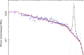
Figure 1: Power spectrum density of XTE J1550–564 as observed by RXTE/PCA on 1998-09-29. Black solid line denotes fitted model composed of double broken power-law model (red solid line) and Lorentzian (dotted line) representing red-noise background spectrum and quasi-periodic oscillation (QPO), respectively. Power spectrum for simulated TK time-series has been marked in blue (circle markers).

Fig. 1 presents Fourier power spectrum density calculated from 78 averaged spectra based on 1024 point data segments. The overall PSD shape can be split into two main components: power-law underlying spectrum and broad line profile representing red-noise source variability and QPO component, respectively. In the $\chi^{2}$ fitting process we found that a model composed of three-segment broken power-law (i.e. with two break frequencies) and Lorentzian profile line [51] fit the PSD best yielding reduced-$\chi^{2}$ of 10.9 at 59 degrees of freedom. The corresponding power-law slope values and break frequencies have been determined as follows: $\alpha_{1}=0.22\pm 0.02,\alpha_{2}=0.90\pm 0.02,\alpha_{3}=3.40\pm 0.07,f_{1}=1.63\pm 0.08$ Hz and $f_{2}=8.12\pm 0.10$, whereas for Lorentzian the central frequency of $f_{0}=4.104\pm 0.006$ Hz and its FWHM $\Delta f=0.33\pm 0.01$ Hz were fitted providing QPO quality factor of $Q\simeq 12.4$. We marked both model components in Fig. 1 by red solid line and dotted line, respectively, where the overall best model has been indicated by black solid line.

Based on the above power-law model we generated a $2^{16}$ point long simulated signal (64 segments of 1024 points) with TK method. In simulation we assumed the sampling time of $\Delta t=2^{-5}$ s and ensured that resulting rms value (here, derived in 0.5–2 Hz and 8–12 Hz frequency band; see Sect. II-B for details) was nearly the same as compared to corresponding rms values for X-ray source. We calculated the averaged Fourier PSD for TK time-series and plotted it in Fig. 1 by blue circle markers. One can clearly notice that TK PSD reproduces well the assumed double broken power-law model component.

Following the recipe given in Section II-C we aim at determination of wavelet confidence at 0.9995 level. From the entire XTE J1550–564 light curve, we select a 3072 point long test signal (96 s) for which we compute wavelet significance matrix (Eq. 20). Upper plot of Fig. 2 presents a dependence of 0.9995-th wavelet quantile (Eq. 18) in a function of Fourier frequency in 1–10 Hz band, both for X-ray data segment (black solid line) and TK simulation (red dashed line). It is straightforward to note that at the significance of $5\times 10^{-4}$ the quasi-periodic variability around $f\simeq 4$ Hz is high above the mean (simulated) red-noise level. Finally, the bottom map of Fig. 2 presents the wavelet power spectrum (Eq. 1) for considered data segment with overlaid contours of derived significance.

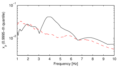
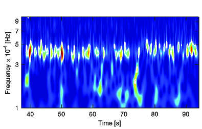
Figure 2: (upper) The dependence of 0.9995-th quantiles in a function of frequency calculated for selected 96 s data signal of XTE J1550–564 (solid black line) and obtained from wavelet analysis of simulated TK series (red dashed line). See Section III-A for details. (bottom) Corresponding wavelet power spectrum displayed with derived significance contours (0.9995 confidence level). For better clarity of map reading we plot 96 s long wavelet spectrum between 37–94 s only.

III-B RE J1034+396

A Seyfert 1 galaxy of RE J1034+396 has been found and confirmed as the first active galaxy showing highly significant quasi-periodic oscillation (QPO) at the frequency $f\simeq 2.7\times 10^{-4}$ Hz [49]. We reproduce their PSD in Fig. 3 as computed for signal segment of XMM-Newton EPIC observation of RE J1034+396 conducted on 2007-05-31. Solid black line crossing PSD denotes best-fitted power-law spectrum described as:

$$\lg P(f)=-1.35\lg f-4.128$$ (21)

(M. Gierlinski, private communication). Upper two dashed lines mark computed confidence levels for detected periodicity at 99.73% ($3\sigma$) and 99.99% confidence levels. In order to verify aforementioned significance of QPO detection, we downloaded from XMM-Newton Science Operations Centre the same EPIC pn+MOS1/MOS2 observation data set and reduced it in the same manner as described in [49]. We limit original X-ray light curve (0.3–10 keV) to 601 point long time-series (corresponding to segment 2 of [49]) where the sampling time of $\Delta t=100$ s has been used.

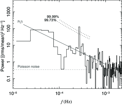
Figure 3: Fourier power spectral density of an active galaxy of RE J1034+396 [49] displaying a significant quasi-periodicity at frequency $f\simeq 2.7\times 10^{-4}$ Hz $(>99.99\%$ of confidence; upper dotted line). Solid line denotes best power-law model fitted to the data $P(f)\propto f^{-1.35}$, whereas bottom horizontal dotted lines marks expected white-noise level. Reproduced with kind permission of Marek Gierlinski.

We compute wavelet power spectrum (1) in $10^{-4}$–$10^{-3}$ Hz band and make use of our new algorithm in order to determine two contour plots marking 99.73% and 99.99% confidence for wavelet results. For the purpose of wavelet background simulation, we generate $2^{16}$ point TK signal based on assumed single power-law model (Eq. 21). Since the underlying PSD model is known in advance, we perform an integration of it between $10^{-4}$ Hz and $10^{-3}$ Hz to find the corresponding rms value in this frequency range (rms$\simeq 5.5$%). Within the simulation process of TK time-series we check to make sure that in the same frequency band the rms of TK signal stays in agreement with derived value. Based on that, we determine two significance matrices (Eq. 20) and plot them together with wavelet power spectrum. The final form of all calculations presents Fig. 4 where an outter and inner contour denote 99.73% and 99.99% confidence level, respectively.

Remarkably, a detected quasi-periodic oscillation at $f\simeq 2.7\times 10^{-4}$ Hz appears to be very coherent in time though showing small but noticeable period drift. We checked that the entire periodicity remains significant at the confidence level of 99% throughout the signal segment duration. In contrast, as marked in Fig. 4, only a small fraction of QPO activity exceeds top level of $0.01\%$ significance whereas about 70% of detected QPO signal stays significant at $3\sigma$ level.

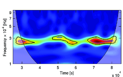
Figure 4: RE J1034+396: Wavelet power spectrum calculated for the second data segment of XMM-Newton EPIC/pn+MOS observation, as defined by [49]. Quasi-periodic modulation is clearly detected at $f\simeq 2.7\times 10^{-4}$ Hz frequency and last throughout a whole light curve duration. Outer and inner contours correspond to derived 99.73% ($3\sigma$) and 99.99% confidence level, respectively, with the use of new algorithm as provided in Section II-C.

IV Conclusions

In this paper we reviewed a recent status of knowledge devoted to wavelet significance tests and proposed a new method designed especially for signals which intrinsic variability displays in Fourier power spectral density a power-law form. Since a large number of astronomical X-ray sources has been found to be characterized by the similar PSD shapes, we focused our attention to that class of objects and their time-series analysis.

We presented a flexible algorithm helpful in determination of the significance of quasi-periodic oscillations in the wavelet domain. Our method has been based on a comparison of wavelet coefficients calculated for X-ray time-series with those computed for simulated signal, where the latter displays the same PSD broad-band model of variability as X-ray object.

We argue that the usefulness of our new algorithm can be easily extended to non-astronomical time-series which PSD can be described by power-law model as well. If required, the omission of exponential transformation of linear signal generated with the use of TK method and inclusion of Poisson noise should be avoided (Section II-A).

References

- [1] R. N. Bracewell, ”The Fourier Transform and Its Applications”, McGraw-Hill, 1965, 2nd ed. 1978, revised 1986
- [2] J. H. Swank, “The XTE Mission”, Bulletin of the American Astronomical Society, vol. 26, pp. 1420, 1994
- [3] C. Gabriel, M. Guainazzi and L. Metcalfe, “XMM-Newton: Passing Five Years of Successful Science Operations”, Astronomical Data Analysis Software and Systems XIV, vol. 347, pp. 425, 2005
- [4] P. Uttley, I. M. McHardy and I. E. Papadakis, “Measuring the broad-band power spectra of active galactic nuclei with RXTE”, Monthly Notices of the Royal Astronomical Society, vol. 332, issue 1, pp. 231-250, 2002
- [5] W. H. G. Lewin and M. van der Klis, “Compact stellar X-ray sources”, Cambridge Astrophysics Series, No. 39. Cambridge, UK: Cambridge University Press, 2006
- [6] R. Sunyaev, and M. Revnivtsev, “Fourier power spectra at high frequencies: a way to distinguish a neutron star from a black hole”, Astronomy and Astrophysics, vol. 358, pp. 617-623, 2000
- [7] N. I. Shakura and R.A. Sunyaev, “Black holes in binary systems. Observational appearance”, Astronomy and Astrophysics, vol. 24, pp. 337, 1973
- [8] C. M. Urry and P. Padovani, “Unified Schemes for Radio-Loud Active Galactic Nuclei”, Publications of the Astronomical Society of the Pacific, vol. 107, p. 803
- [9] M. van der Klis, “Neutron Star QPOs as Probes of Strong Gravity and Dense Matter”, X-ray Timing 2003: Rossie and Beyond. AIP Conference Proceedings, vol. 714, pp. 371-378, 2004
- [10] J. Frank, A. King A. and D. J. Raine, “Accretion Power in Astrophysics”, Cambridge University Press, 2002
- [11] C. Done and M. Gierliński, “Observing the effects of the event horizon in black holes”, Monthly Notice of the Royal Astronomical Society, vol. 342, issue 4, pp. 1041-1055, 2003
- [12] K. Pottschmidt, J. Wilms, M. A. Nowak, G. G. Pooley, T. Gleissner, W. A. Heindl, D. M. Smith, R. Remillard and R. Staubert, “Long term variability of Cygnus X-1. I. X-ray spectral-temporal correlations in the hard state”, Astronomy and Astrophysics, vol. 407, pp. 1039-1058, 2003
- [13] A. Lawrence, M. G. Watson, K. A. Pounds,and M. Elvis, “Low-frequency divergent X-ray variability in the Seyfert galaxy NGC4051”, Nature, vol. 325, p. 694, 1987
- [14] I. M. McHardy, I. E. Papadakis, P. Uttley, M. J. Page and K. O. Mason, “Combined long and short time-scale X-ray variability of NGC 4051 with RXTE and XMM-Newton”, Monthly Notices of the Royal Astronomical Society, vol. 348, issue 3, pp. 783-801, 2004
- [15] T. Belloni and G. Hasinger, “Variability in the noise properties of Cygnus X-1”, Astronomy and Astrophysics, vol. 227, no. 2, L33-L36, 1990
- [16] M. A. Nowak, B. A. Vaughan, J. Wilms, J. B. Dove and M. C. Begelman, “Rossi X-Ray Timing Explorer Observation of Cygnus X-1. II. Timing Analysis”, The Astrophysical Journal, vol. 510, issue 2, pp. 874-891, 1999
- [17] W. Press, ”Flicker noises in astronomy and elsewhere”, Comments on Astrophysics, vol. 7, p. 103, 1978
- [18] M. van der Klis, “The QPO phenomenon”, Astronomische Nachrichten, vol. 326, issue 9, p.798-803, 2005
- [19] M. van der Klis, “Comparing Black Hole and Neutron Star Variability”, Astrophysics and Space Science, vol. 300, issue 1-3, pp. 149-157, 2005
- [20] L. Cohen, “Time-frequency analysis”, Englewood Cliffs, NJ: Prentice-Hall, 1995
- [21] J. Wilms, M. A. Nowak, K. Pottschmidt, W. A. Heindl, J. B. Dove and M. C. Begelman, “Discovery of recurring soft-to-hard state transitions in LMC X-3”, Monthly Notices of the Royal Astronomical Society, vol. 320, issue 3, pp. 327-340, 2001
- [22] D. Barret, W. Kluźniak, J. F. Olive, S. Paltani and G. K. Skinner, “On the high coherence of kHz quasi-periodic oscillations”, Monthly Notices of the Royal Astronomical Society, vol. 357, issue 4, pp. 1288-1294, 2005
- [23] Y. Meyer and S. Roques, “Progress in wavelet analysis and applications”, 1993, Proceedings of the International Conference ”Wavelets and Applications”, Toulouse, France, June 1992, Gif-sur-Yvette: Editions Frontieres, ed. by Meyer, Yves; Roques, Sylvie, 1993
- [24] P. S. Addison, “Illustrated Wavelet Transform Handbook”, IoP, 2002
- [25] P. Lachowicz and B. Czerny, “Wavelet analysis of millisecond variability of Cygnus X-1 during its failed state transition”, Monthly Notices of the Royal Astronomical Society, vol. 361, issue 2, pp. 645-658, 2005
- [26] C. Torrence and G. P. Compo, “A Practical Guide to Wavelet Analysis”, Bulletin of the American Meteorological Society, vol. 79, issue 1, pp. 61-78, 1998
- [27] S. Vaughan, R. Edelson, R. S. Warwick and P. Uttley, “On characterizing the variability properties of X-ray light curves from active galaxies”, Monthly Notices of the Royal Astronomical Society, vol. 345, issue 4, pp. 1271-1284, 2003
- [28] M. van der Klis, “Quasi-periodic oscillations and noise in low-mass X-ray binaries”, Annual review of astronomy and astrophysics. Volume 27. Palo Alto, CA, Annual Reviews, Inc., pp. 517-553, 1989
- [29] D. L. Gilman, F. J. Fuglister and J. M. Mitchell Jr., “On the Power Spectrum of Red Noise”, Journal of Atmospheric Sciences, vol. 20, issue 2, pp. 182-184, 1963
- [30] S. L. Marple, Jr., “Digital Spectral Analysis with Applications”, Prentice Hall, Englewood Cliffs, 1987, Chapter 8
- [31] C. Chatfield, “The Analysis of Time Series. An Introduction.”, Chapman & Hall, A CRC Press Company, Sixth Ed., 2004
- [32] S. M. Kay, “Modern Spectral Estimation: Theory and Application”. Englewood Cliffs, NJ: Prentice-Hall, 1988
- [33] P. Uttley, I. M. McHardy and S. Vaughan, “Non-linear X-ray variability in X-ray binaries and active galaxies”, Monthly Notices of the Royal Astronomical Society, vol. 359, p. 345, 2005
- [34] K. Pottschmidt, M. Koenig, J. Wilms and R. Staubert, “Analyzing short-term X-ray variability of Cygnus X-1 with Linear State Space Models”, Astronomy and Astrophysics, vol. 334, p. 201, 1998
- [35] Z. Ge, “Significance test for wavelet power and the wavelet power spectrum”, Ann. Geophys. , vol. 25, p. 2259, 2007
- [36] D. Maraun and J. Kurths, “Cross Wavelet Analysis. Significance Testing and Pitfalls”, Nonlin. Proc. Geoph., vol. 11(4), pp. 505-514, 2004
- [37] D. Maraun, J. Kurths and M. Holschneider, “Nonstationary Gaussian processes in wavelet domain: Synthesis, estimation, and significance testing”, Physical Review E, vol. 75, issue 1, id. 016707, 2007
- [38] G. F. Smoot, et al., “Structure in the COBE differential microwave radiometer first-year maps”, Astrophysical Journal, vol. 396, L1 , 1992
- [39] R. Fabbri and S. Torres, “Peak statistics on COBE maps”, Astronomy and Astrophysics, vol. 307, pp. 703-707, 1996
- [40] J. Timmer and M. Koenig, “On generating power law noise”, Astronomy and Astrophysics, vol. 300, p. 707, 1995
- [41] P. Uttley and I. M. McHardy, “The flux-dependent amplitude of broadband noise variability in X-ray binaries and active galaxies”, Monthly Notices of the Royal Astronomical Society, vol. 323, L26, 2001
- [42] W. H. Press, S. A. Teukolsky, W. T. Vetterling W.T. and B. P. Flannery B.P., “Numerical recipes in FORTRAN. The art of scientific computing”, Cambridge: University Press, 2nd ed., 1992
- [43] M. van der Klis, “Quantifying Rapid Variability in Accreting Compact Objects”, Statistical Challenges in Modern Astronomy II, 321, 1997
- [44] Ch. Clapham, The Concice Oxford Dictonary of Mathematics, Oxford University Press, 1996
- [45] D. A. Smith, “XTE J1550-564”, IAU Circ., 7008, 1, 1998
- [46] J. A. Orosz, et al. “Dynamical Evidence for a Black Hole in the Microquasar XTE J1550-564”, The Astrophysical Journal, vol. 568, p. 845, 2002
- [47] W. Cui, S. N. Zhang, W. Chen and E. H. Morgan, “Strong aperiodic X-ray variability and quasi-periodic oscillationin X-ray nova XTE J1550-564, The Astrophysical Journal Letters, vol. 512, L43, 1999
- [48] R. A. Remillard, J. E. McClintock, G. J. Sobczak, C. D. Bailyn, J. A. Orosz, E. H. Morgan and A. M. Levine, “X-Ray Nova XTE J1550-564: Discovery of a Quasi-periodic Oscillation near 185 Hz”, The Astrophysical Journal Letters, vol. 517, L127, 1999
- [49] M. Gierliński, M. Middleton, M. Ward, and C. Done, “A periodicity of 1hour in X-ray emission from the active galaxy RE J1034+396”, Nature, vol. 455, issue 7211, pp. 369-371, 2008
- [50] A. A. Zdziarski and M. Gierliński, “Radiative Processes, Spectral States and Variability of Black-Hole Binaries”, Progress of Theoretical Physics Supplement, No. 155, pp. 99-119, 2004
- [51] K. A. Arnaud, K.A., Astronomical Data Analysis Software and Systems V, eds. Jacoby G. and Barnes J., p. 17, ASP Conf. Series vol. 101, 1996