Dynamical regimes and hydrodynamic lift of viscous vesicles under shear

Abstract

The dynamics of two-dimensional viscous vesicles in shear flow, with different fluid viscosities $\eta_{\rm in}$ and $\eta_{\rm out}$ inside and outside, respectively, is studied using mesoscale simulation techniques. Besides the well-known tank-treading and tumbling motions, an oscillatory swinging motion is observed in the simulations for large shear rate. The existence of this swinging motion requires the excitation of higher-order undulation modes (beyond elliptical deformations) in two dimensions. Keller-Skalak theory is extended to deformable two-dimensional vesicles, such that a dynamical phase diagram can be predicted for the reduced shear rate and the viscosity contrast $\eta_{\rm in}/\eta_{\rm out}$. The simulation results are found to be in good agreement with the theoretical predictions, when thermal fluctuations are incorporated in the theory. Moreover, the hydrodynamic lift force, acting on vesicles under shear close to a wall, is determined from simulations for various viscosity contrasts. For comparison, the lift force is calculated numerically in the absence of thermal fluctuations using the boundary-integral method for equal inside and outside viscosities. Both methods show that the dependence of the lift force on the distance $y_{\rm{cm}}$ of the vesicle center of mass from the wall is well described by an effective power law $y_{\rm{cm}}^{-2}$ for intermediate distances $0.8R_{\rm p}\lesssim y_{\rm{cm}}\lesssim 3R_{\rm p}$ with vesicle radius $R_{\rm p}$. The boundary-integral calculation indicates that the lift force decays asymptotically as $1/[y_{\rm{cm}}\ln(y_{\rm{cm}})]$ far from the wall.

I Introduction

Vesicles are fluid droplets enclosed by a fluid lipid membrane. Typically, vesicles have sizes of the order of 100 nanometers to 10 micrometers, whereas the thickness of the membrane is only of the order of a nanometer. Therefore, the membrane can often be regarded as a two-dimensional manifold. Vesicle shapes and fluctuations are then governed by the curvature elasticity. This description has been very successful to explain vesicles behavior in thermal equilibrium Seifert (1997).

The dynamics of fluid vesicles in shear flow has attracted much attention recently Keller and Skalak (1982); Kraus et al. (1996); Beaucourt et al. (2004); Noguchi and Gompper (2004, 2005); Noguchi (2009); Pozrikidis (2001); de Haas et al. (1997); Kantsler and Steinberg (2005, 2006); Mader et al. (2006); Misbah (2006); Vlahovska and Gracia (2007); Noguchi and Gompper (2007); Danker et al. (2007); Lebedev et al. (2007, 2008). Aspherical vesicles under shear can be found in different dynamical phases, depending on the viscosities $\eta_{\rm{in}}$ and $\eta_{\rm{out}}$ of inner and outer fluids, respectively, the membrane viscosity $\eta_{\rm{mb}}$, the bending rigidity $\kappa$, the shear rate $\dot{\gamma}$, the membrane area, and enclosed volume. As long as shape relaxation times of the vesicle are small compared to the time scale set by the shear rate $\dot{\gamma}$, the vesicle is always close to its equilibrium shape. Under these conditions, vesicles can be found either in tank-treading (TT) motion, or – if the viscosity contrast $\lambda=\eta_{\rm{in}}/\eta_{\rm{out}}$ exceeds a critical value – in a tumbling (TB) motion. In the tank-treading regime, the vesicle shape and orientation are stationary in time, but the membrane rotates around the vesicle’s center of mass in the same direction as the rotational part of the shear flow. Here, the orientation is characterized by the inclination angle $\theta$ with respect to the flow direction. In the tumbling regime, the long axis of the vesicle performs a periodic rotation. Keller and Skalak Keller and Skalak (1982) developed a theory for fluid vesicles with fixed ellipsoidal shape and different viscosity contrasts, which is able to explain the observed experiments. In recent years, computer simulations Kraus et al. (1996); Beaucourt et al. (2004); Noguchi and Gompper (2004, 2005); Noguchi (2009) have shown that the Keller-Skalak (KS) theory provides indeed a very good description of tank-treading and tumbling.

However, the vesicle dynamics is far less understood when the shear rate is large enough that the vesicle cannot relax into its equilibrium shape. Only recently, it was shown that a third dynamical regime can appear under these conditions, the swinging (SW) regime Kantsler and Steinberg (2006); Mader et al. (2006); Misbah (2006); Vlahovska and Gracia (2007); Noguchi and Gompper (2007); Danker et al. (2007); Lebedev et al. (2007, 2008) — also called the trembling Kantsler and Steinberg (2006) or vacillating-breathing regime Misbah (2006). In the swinging state, oscillations of shape and inclination angle together determine the vesicle dynamics. Swinging vesicles were first observed experimentally in Ref. Kantsler and Steinberg (2006). With increasing shear rate, a transition from tumbling to swinging motion was found. A perturbation theory for quasi-spherical vesicles to lowest order in the deviation from the spherical shape predicted swinging for a range of viscosity contrasts Misbah (2006); however, since the shear rate appears only as basic (inverse) time scale in this approach, the experimental results could not be explained. Therefore, higher-order expansions for quasi-spherical vesicles Danker et al. (2007); Lebedev et al. (2007, 2008) and a generalized Keller-Skalak (KS) theory for ellipsoidal vesicles Noguchi and Gompper (2007) have been developed, which are able to predict phase transitions with varying shear rate and thereby to explain the experiments of Ref. Kantsler and Steinberg (2006).

The dynamics in the TT, TB, and SW phases has been studied mainly for single vesicles in an unbounded fluid. However, in particular due to its physiological importance, it is of high interest to study the dynamical behavior of vesicles under shear in the presence of walls. In this case, vesicles are repelled from a wall due to a hydrodynamic lift force $F_{\rm L}$. The hydrodynamic lift force plays an important role in circulatory systems of vertebrates. Since the lift force pushes red blood cells to the center of a blood vessel, where the flow velocity is largest, it increases the efficiency of oxygen transport. On the other hand, white blood cells move along the vessel walls in order to find defects in the vascular endothelium Fung (1997); Imhof and Dunon (1997). This is achieved by special ligands, which are located at the outside of white blood cells and bind to receptors on the vessel wall to resist the hydrodynamic lift force Chang et al. (2000); Dwir et al. (2003).

The existence of a hydrodynamic lift force was first reported by Poiseuille in 1836 Poiseuille (1836), who observed this effect on blood cells. In recent years, the hydrodynamic lift force was studied intensively, both theoretically Olla (1997a, b); Cantat and Misbah (1999); Seifert (1999); Sukumaran and Seifert (2001) and experimentally Lorz et al. (2000); Abkarian et al. (2002); Abkarian and Viallat (2005); Callens et al. (2008). Abkarian et al. Abkarian et al. (2002); Abkarian and Viallat (2005) observed the unbinding of a heavy vesicle, which was pulled by gravity towards a wall, with increasing shear rate. For vesicles which are not in direct contact with the wall, only studies in three dimensions with equal viscosities of inside and outside fluids exist. Both, boundary-integral simulations Sukumaran and Seifert (2001) as well as theoretical studies Olla (1997a, b) show that the lift force decays with a power law $1/y^{2}_{\rm{cm}}$ with increasing distance between the vesicle’s center of mass and the wall. For vesicles in two dimensions, there are only theoretical and numerical studies which focus on adhering vesicles bound to the wall by a short-ranged attractive potential Cantat and Misbah (1999); Seifert (1999).

In this paper, we study the dynamics of a two-dimensional ($2$D) vesicle as a function of viscosity contrast $\lambda$ and shear rate $\dot{\gamma}$, both in the bulk and near a wall. The advantage of simulations of a vesicle in two dimensions is (i) the reduced numerical effort of hydrodynamics simulations, which allows for larger system sizes, longer accessible time scales, and better statistics, and (ii) the simpler form of the equations of the KS theory, where no integrals remain in the geometric factors – unlike in the $3$D version (see App. A). This facilitates a detailed comparison of the results of theory and simulations. Using a mesoscopic hydrodynamics approach, we first show that the SW mode also exists in two dimensions, and determine the dynamical phase diagram. The simulation results are compared with the predictions of a generalized KS theory. Second, we study the lift force $F_{\rm L}$ of $2$D vesicles, by covering the full range of wall distances $y_{\rm{cm}}$, and investigate the effects of viscosity contrast $\lambda$. Moreover, we investigate the effect of a wall on the TT-TB behavior. For comparison with the results of mesoscopic hydrodynamics simulations, we also determine $F_{\rm L}$ and the inclination angle $\theta$ by the boundary-integral method for tank-treading vesicles with $\lambda=1$.

II Theory and Methods

II.1 Dimensionless Parameters

In a $2$D vesicle, the perimeter $L_{\rm p}$ and the enclosed area $A$ are kept constant (analogously to the constant membrane surface and the enclosed volume of $3$D vesicles). It is useful to combine these two parameters into a dimensionless quantity, the reduced area

$$A^{*}:=\frac{4\pi A}{{L_{\rm p}}^{2}}=\Big{(}\frac{R_{\rm A}}{R_{\rm p}}\Big{)}^{2}.$$ (1)

Here $R_{\rm p}=L_{\rm p}/2\pi$ and $R_{\rm A}=\sqrt{A/\pi}$ are the radii of circles with the same $L_{\rm p}$ and $A$ as those of the vesicle, respectively. $A^{*}$ is the ratio between the enclosed area $A$ and the area of a circle with the same perimeter $L_{\rm p}$. We focus here on a reduced area of $A^{*}=0.7$ as a representative for vesicles which deviate significantly from the circular shape.

Shape and orientation of the vesicles are quantified by a shape parameter $\alpha$ and inclination angle $\theta$ based on the gyration tensor of the vesicle membrane. When $\Lambda_{\rm{max}}$ and $\Lambda_{\rm{min}}$ are the two eigenvalues of the gyration tensor ($\Lambda_{\rm{max}}\geq\Lambda_{\rm{min}}$), and ${\bf\hat{e}}_{\rm{max}}$ and ${\bf\hat{e}}_{\rm{min}}$ the corresponding eigenvectors, the “asphericity” is described by $\alpha=(\Lambda_{\rm{max}}-\Lambda_{\rm{min}})/(\Lambda_{\rm{max}}+\Lambda_{\rm{min}})$ and the vesicle orientation by the inclination angle $\theta=\measuredangle({\bf\hat{x}},{\bf\hat{e}}_{\rm{max}})$, where ${\bf\hat{x}}$ is the shear and ${\bf\hat{y}}$ the gradient direction.

The stability of dynamical phases mainly depends on two parameters, the viscosity contrast $\lambda$ and the reduced shear rate

$$\dot{\gamma}^{*}:=\frac{\dot{\gamma}\eta_{\rm{out}}R_{\rm p}^{3}}{\kappa}.$$ (2)

The time $\eta_{\rm{out}}R_{\rm p}^{3}/\kappa$ is the characteristic relaxation time in thermal equilibrium, where $\kappa$ is the bending rigidity. Thus $\dot{\gamma}^{*}$ expresses the interplay between the perturbation by the external field $\dot{\gamma}$ and the ability of the vesicle to restore its equilibrium shape.

II.2 Generalized Keller-Skalak Theory in Two Dimensions

Keller-Skalak (KS) theory Keller and Skalak (1982) is based on the assumption that vesicles have a fixed ellipsoidal shape. Therefore, it cannot describe the swinging state with oscillating vesicle shapes. Therefore, KS theory has been generalized to include shape deformation in three dimensions Noguchi and Gompper (2007). This theory is applicable to ellipsoidal vesicles over a wide range of reduced volumes, while higher-order perturbation theory Danker et al. (2007); Lebedev et al. (2007, 2008) is limited to quasi-spherical vesicles. Here, we employ the two-dimensional version of the generalized KS theory. The differential equations for the asphericity $\alpha$ and inclination angle $\theta$ are given by

$$\frac{1}{\dot{\gamma}}\frac{d\alpha}{dt} = -\frac{b_{0}}{A^{*}\dot{\gamma}^{*}}\frac{R_{\rm p}}{\kappa}\frac{\partial F}{\partial\alpha}+b_{1}\sin(2\theta),$$ (3)

$$\frac{1}{\dot{\gamma}}\frac{d\theta}{dt} = \frac{1}{2}\left[-1+B(\alpha)\cos(2\theta)\right],$$ (4)

with prefactors

$$b_{0}=\frac{3}{4\pi(\lambda+1)}\ \ \ \mathrm{and}\ \ \ b_{1}=\frac{3}{2(\lambda+1)}.$$ (5)

There are no adjustable parameters. An explicit expression for $B(\alpha)$ and its derivation are described in App. A.

The time evolution of $\theta$ is described by Eq. (4), which has the same form as in two-dimensional KS theory. However, $B(\alpha)$ is now not constant but depends on the time-dependent vesicle shape $\alpha(t)$. The time evolution of $\alpha$ (see Eq. (3)) is derived based on the perturbation theory of quasi-circular vesicles Finken et al. (2008). Here, $F$ is the free energy of the vesicle shape at constant $A^{*}$. $F$ attains its minimum for an elliptical vesicle shape in equilibrium. Thus, the first term on the right hand side of Eq. (3) causes a relaxation of $\alpha$ towards its equilibrium value. The second term represents the change of $\alpha$ due to the external flow field. Eqs. (3) and (4) are solved numerically using a fourth-order Runge-Kutta method.

Thermal fluctuations can be incorporated in this approach by adding Gaussian white noises $g_{\alpha}(t)$ and $g_{\theta}(t)$ to Eqs. (3) and (4), respectively. The noise terms obey the fluctuation-dissipation theorem, such that $\left<g_{i}(t)\right>=0$ and $\left<g_{i}(t)g_{j}(t^{\prime})\right>=(2k_{\rm B}T/\zeta_{i})\delta_{i,j}\delta(t-t^{\prime})$ with $i,j\in\{\alpha,\theta\}$, where $k_{\rm B}T$ is the thermal energy. As a reasonable approximation, we employ the rotational friction coefficients of a circle,

$$\zeta_{\alpha}=\frac{4\pi}{3}\eta_{\rm{out}}{R_{\rm A}}^{2}(\lambda+1)\ \ \mathrm{and}\ \ \zeta_{\theta}=4\pi\eta_{\rm{out}}{R_{\rm p}}^{2}.$$ (6)

II.3 Mesoscale Hydrodynamics Simulation Method

II.3.1 Membrane Model

The membrane is modeled by a closed chain of $n$ monomers of mass $M$. For a monomer with index $i$ (with $1\leq i\leq n$), we introduce the notation

$$i_{-}=(i-1)\,\mathrm{mod}\,n\qquad\mathrm{and}\qquad i_{+}=(i+1)\,\mathrm{mod}\,n$$ (7)

for the indices of its two neighboring monomers. Thereby, the ring topology is taken into account correctly. The monomers are connected by a harmonic spring potential

$$U_{\rm{sp}}=\frac{k_{\rm{sp}}}{2}\sum^{n}_{i=1}(|{\bf R}_{i}|-l)^{2},$$ (8)

where ${\bf R}_{i}:={\bf r}_{i_{+}}-{\bf r}_{i}$ are the bond vectors, and $l$ is the relaxed bond length. The curvature elasticity of the membrane is described by the bending potential

$$U_{\rm{bend}}=\frac{\kappa}{l}\sum^{n}_{i=1}\left(1-\frac{{\bf R}_{i_{+}}\cdot{\bf R}_{i}}{|{\bf R}_{i_{+}}\parallel{\bf R}_{i}|}\right).$$ (9)

An area potential

$$U_{\rm A}=\frac{k_{\rm A}}{2}\left(A-A_{0}\right)^{2}.$$ (10)

is introduced to control the deviations of the area $A$ from its target value $A_{0}$. Here, the enclosed area $A$ in Eq. (10) is obtained from the monomer positions by

$$A=\frac{1}{2}{\bf\hat{z}}\cdot\sum^{n}_{i=1}{\bf r}_{i}\times{\bf r}_{i_{+}}.$$ (11)

II.3.2 Multi-Particle Collision Dynamics

For the solvent hydrodynamics, we employ multi-particle collision dynamics (MPC), a particle-based mesoscopic simulation technique Malevanets and Kapral (1999); Kapral (2008); Gompper et al. (2009). The dynamics of an MPC fluid evolves in two alternating steps. In the “streaming step”, particles move ballistically for a time $\Delta t$, the collision time, according to their current velocities. For the “collision step”, solvent particles are first sorted into the cells of linear size $a$ of a regular square lattice; all particles in a cell then exchange momenta such that the total translational momentum is conserved in each collision cell.

Several modifications of the original MPC algorithm have been introduced recently Noguchi et al. (2007), which differ in the way the collision step is executed. We employ the MPC-AT$+a$ version of multi-particle collision dynamics, which uses an Anderson thermostat (AT) and locally conserves angular momentum ($+a$) in addition to translational momentum. In MPC-AT, new particle velocities relative to the center-of-mass velocity are chosen from a Maxwell-Boltzmann distribution with temperature $T$. This thermostat avoids any heating due to energy dissipation in sheared system. For details of the MPC-AT$+a$ algorithm, see Refs. Noguchi et al. (2007); Noguchi and Gompper (2008). We use this algorithm, since local angular-momentum conservation is crucial in binary fluid systems with different viscosities Götze et al. (2007).

Simulations are performed with a rectangular simulation box with linear sizes $L_{x}$ and $L_{y}$, periodic boundary conditions in the $x$ direction, and no-slip wall boundary conditions in the $y$ direction. Linear shear flow with shear rate $\dot{\gamma}$ is realized by moving the upper wall with a velocity $\dot{\gamma}L_{y}{\bf\hat{x}}$, whereas the lower wall is held at rest.

Many properties of the MPC-AT$+a$ solvent can be adjusted by the simulation parameters collision time $\Delta t$, the particle number density $n_{\rm s}$, and the particle mass $m$. The solvent viscosity $\eta=\eta_{\rm{kin}}+\eta_{\rm{coll}}$ is a sum of a kinetic $\eta_{\rm{kin}}$ and a collisional contribution $\eta_{\rm{coll}}$, which have been calculated analytically Noguchi and Gompper (2008),

$$\eta_{\rm{kin}} = \frac{n_{\rm s}k_{\rm B}T\Delta t}{a^{2}}\left[\frac{n_{\rm s}}{n_{\rm s}-1}-\frac{1}{2}\right],$$ (12)

$$\eta_{\rm{col}} = \frac{m(n_{\rm s}-7/5)}{24\Delta t}.$$ (13)

The viscosity $\eta_{\rm{out}}$ of the fluid outside of the vesicle is adjusted by varying the collision time $\Delta t$ in the range from $\Delta t=0.003a\sqrt{m/k_{\rm B}T}$ to $\Delta t=0.01a\sqrt{m/k_{\rm B}T}$. Since for these collision times the mean free path is much smaller than the cell size $a$, the total shear viscosity $\eta$ is dominated by $\eta_{\rm{coll}}$ (see Eqs. (12) and (13)). Since the collisional viscosity $\eta_{\rm{coll}}\propto m$, the viscosity contrast $\lambda$ can be varied by using different masses $m_{\rm{in}}$ and $m$ of the inner and outer fluid particles, respectively, which implies

$$\lambda=\frac{\eta_{\rm{in}}}{\eta_{\rm{out}}}\approx\frac{m_{\rm{in}}}{m}.$$ (14)

In our simulations, the viscosity contrast is varied from $\lambda=1$ to $\lambda=10$ (with $m\leq m_{\rm{in}}\leq 10m$), while all the other MPC parameters are the same for the fluid on both sides of the membrane.

II.3.3 Membrane Interactions

In order to describe an impermeable membrane in flow, it has to be ensured that MPC particles stay on the correct side of the membrane (i.e. inside or outside of the vesicle). For numerical efficiency, it is advantageous to relax this condition for short length and time scales, as it was done in previous $3$D vesicle simulations Noguchi and Gompper (2005). The streaming and collision steps for the fluid particles are carried as in the absence of the membrane. This implies that after each streaming step, some MPC particles have crossed the membrane. For the (few) particles which are now located on the wrong side of the membrane, with a direction of their velocity which would bring them away even further away from the membrane, the velocities have to be modified such that they move towards the membrane instead, in order to cross back to their correct side. We denote this velocity update a “membrane collision”. It has to be constructed such that the translational and angular momentum as well as the kinetic energy of the fluid particles and membrane monomers are conserved locally. Our procedure for membrane collisions is a generalization of the standard bounce-back rule for no-slip boundary conditions. A detailed description of this procedure is provided in App. B.

In order to prevent the membrane from crossing the walls, a purely repulsive Lennard-Jones potential

$$U_{\rm w}(y)\!=\!\left\{\!\begin{array}[]{ll}4\varepsilon\left[\left(\frac{\sigma}{y}\right)^{12}-\left(\frac{\sigma}{y}\right)^{6}\right]+\varepsilon,&0\leq y\leq\sqrt[6]{2}\sigma\\ 0,&\mathrm{otherwise}\\ \end{array}\right.$$

is employed, which depends only on the distance $y$ of a monomer from a wall.

For the determination of hydrodynamic lift forces, we employ a gravitational body force ${\bf f}_{\rm G}=-{\bf\hat{y}}g\Delta\varrho$, which acts on the internal fluid of the vesicle. Here, $g$ denotes the strength of the gravitational field, and $\Delta\varrho$ is the mass-density difference between the inner and outer fluids. The gravitational body force ${\bf f}_{\rm G}$ acting on the inner fluid can be expressed as a potential $U_{\rm G}$, which only depends on the monomer positions,

$$U_{\rm{G}}=\frac{F_{\rm G}}{6A}\sum_{i}\left(y_{i}+y_{i_{+}}\right)\left({\bf r}_{i}\times{\bf r}_{i_{+}}\right)\cdot{\bf\hat{z}}.$$ (15)

Here, $y_{i}$ and $y_{i_{+}}$ are the $y$ components of the monomer positions ${\bf r}_{i}$ and ${\bf r}_{i_{+}}$, respectively, and $F_{\rm G}=\left|\int_{A}{\bf f}_{\rm G}dA\right|$ is the total gravitational force acting on the vesicle. $F_{\rm G}$ has a constant value and is used as a simulation parameter.

As long as not specified otherwise, the parameters used in our vesicle simulations are $n=50$, $l=a=\sqrt[6]{2}\sigma$, $n_{\rm s}=10a^{-2}$, $M=10m$, $\varepsilon=10k_{\rm B}T$, and $\kappa/l=50k_{\rm B}T$. For the reduced area, we require that it deviates less than $1\%$ from its target value of $A^{*}=0.7$. Since $A^{*}$ is a function of the perimeter $L_{\rm p}$ and the enclosed area $A$ (see Eq. (1)), the parameters $k_{\rm{sp}}$ and $k_{\rm A}$ for the potentials $U_{\rm{sp}}$ and $U_{\rm A}$, respectively, have to be sufficiently large. We chose $k_{\rm{sp}}=10^{4}k_{\rm B}T/a^{2}$ and $k_{\rm A}=80k_{\rm B}T/a^{4}$. With these parameters, the effective vesicle radius is obtained to be $R_{\rm p}=7.8\,l$. The size of the simulation box is $L_{x}=L_{y}=80a$. Gravitational forces $F_{\rm G}$ are only applied in simulations for the hydrodynamic lift force, where values in the range $k_{\rm B}T/a\leq F_{\rm G}\leq 50k_{\rm B}T/a$ are investigated.

In simulations, different reduced shear rates $\dot{\gamma}^{*}$ can be achieved, according to Eq. (2), by varying $\dot{\gamma}$, $\eta_{\rm{out}}$, $R_{\rm p}$, or $\kappa$. Since equilibrium properties like the undulation spectrum depend on $R_{\rm p}$ and $\kappa$, we vary $\dot{\gamma}^{*}$ by adjusting $\dot{\gamma}$ and $\eta_{\rm{out}}$. In order to avoid inertial effects, we restrict the shear rates to obtain low Reynolds numbers Re $=\dot{\gamma}\rho R_{\rm p}^{2}/\eta_{\rm{out}}$, where $\rho$ is the density of the outer fluid. The maximum Reynolds number is Re$=0.17$.

II.4 Boundary-Integral Method

For comparison with our MPC simulation results of the lift force, we also perform numerical boundary-integral calculations. The hydrodynamic lift force in $2$D has been studied previously with the boundary-integral approach for vesicles in direct contact with the wall Cantat and Misbah (1999); Seifert (1999). This method has the advantage that it can be used to calculate lift forces on vesicles even for very large distances $y_{\rm{cm}}$ from the wall and for reduced areas $A^{*}$ close to unity, which are not easily accessible by MPC simulations. On the other hand, our boundary-integral calculation is restricted to elliptical shapes and ignores thermal fluctuations, which give rise, e.g., to undulation-induced repulsion near a wall. We focus on tank-treading elliptical vesicles without viscosity contrast, i.e. $\lambda=1$. In the steady tank-treading state the lift force can calculated from a single, time-independent vesicle shape. Whereas in MPC simulations, the wall distance $y_{\rm{cm}}$ is calculated for a given strength of the gravitational force, we follow the opposite procedure with the boundary-integral approach, by calculating the lift force for a given wall distance $y_{\rm{cm}}$.

For ellipse half axes $a_{1}$ and $a_{2}$, wall distance $y_{\rm{cm}}$, and inclination angle $\theta$, the location ${\bf r}$ of the vesicle membrane is uniquely defined (with $x_{\rm{cm}}\equiv 0$). With a parameterization by the angle $\varphi$, it is

$${\bf r}(\varphi)=y_{\rm{cm}}{\bf\hat{y}}+\left(\begin{array}[]{cc}\cos\theta&-\sin\theta\\ \sin\theta&\cos\theta\end{array}\right){\bf r}^{\prime}(\varphi)$$ (16)

where ${\bf r}^{\prime}(\varphi)$ is the membrane position in the principal-axis system of the ellipse,

$${\bf r}^{\prime}(\varphi)=\left(\begin{array}[]{c}a_{1}\cos\varphi\\ a_{2}\sin\varphi\end{array}\right).$$ (17)

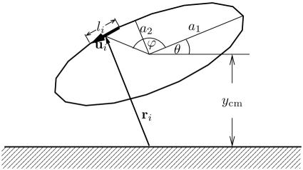
Figure 1: For the boundary-integral calculation, the vesicle is discretized into segments $i$ of length $l_{i}$, which have the orientation ${\bf\hat{u}}_{i}$ and a center-of-mass position ${\bf r}_{i}$.

In the steady tank-treading state, the center-of-mass velocity ${\bf v}_{\rm{cm}}={\bf\hat{x}}v_{\rm{cm}}$ of the vesicle has only a non-vanishing component in shear direction. If $v_{\rm{cm}}$ and the tank-treading angular velocity $\omega$ are known, the velocity of the tank-treading membrane is given by

$${\bf v}(\varphi)={\bf\hat{x}}v_{\rm{cm}}+{R_{\rm p}\omega}{\bf\hat{t}}(\varphi).$$ (18)

with the tangent vector

$${\bf\hat{t}}(\varphi)=\left(\begin{array}[]{cc}\frac{a_{2}}{a_{1}}\sin\theta&\frac{a_{1}}{a_{2}}\cos\theta\\ -\frac{a_{2}}{a_{1}}\cos\theta&\frac{a_{1}}{a_{2}}\sin\theta\end{array}\right)\frac{{\bf r}^{\prime}(\varphi)}{\left|{\bf r}^{\prime}(\varphi)\right|}.$$ (19)

In a tank-treading membrane in shear flow, forces arising from pressure and viscous stress have to be balanced in order to maintain a steady motion. The force distribution ${\bf f}({\bf r}^{\prime})$ along the membrane $\partial A$ is related to the velocity field at position ${\bf r}$ by

$${\bf v}({\bf r})-\dot{\gamma}y{\bf\hat{x}}=\int_{\partial A}\mathbf{G}({\bf r},{\bf r}^{\prime}(s)){\bf f}({\bf r}^{\prime}(s))ds.$$ (20)

Here, $ds$ is a line element of the membrane $\partial A$, and the second-order tensor $\mathbf{G}({\bf r},{\bf r}^{\prime}(s))$ is the Greens function of the Stokes equation which satisfies the boundary conditions. For vesicles in an unbounded fluid, $\mathbf{G}({\bf r},{\bf r}^{\prime}(s))$ is the Oseen tensor. In our case of a vesicle near a wall, the half-space Oseen tensor – also known as Blake tensor – is convenient, as it realizes no-slip boundary conditions at the wall. The full expression for the two-dimensional Blake tensor can be found in Ref. Pozrikidis (1992).

The difficulty is that the force distribution ${\bf f}({\bf r}^{\prime})$ along the membrane is a priori unknown. Instead, we know the velocities ${\bf v}({\bf r})$ at each site of the membrane. Eq. (20) is thereby a Fredholm integral equation of the first type. This integral equation is solved numerically. For this purpose, we discretize the membrane in $N$ straight segments, which have to be small enough such that the difference in velocities between two neighboring segments is small and the force distribution can be assumed to be constant along the segment. A segment with index $i$ has a velocity ${\bf v}_{i}$, center-of-mass position ${\bf r}_{i}$, length $l_{i}$ and orientation ${\bf\hat{u}}_{i}$ (see Fig. 1). The discretized form of Eq. (20) is

$${\bf v}_{i}-\dot{\gamma}y_{i}{\bf\hat{x}}=\sum_{j=1}^{N}\int_{-l_{j}/2}^{l_{j}/2}\mathbf{G}({\bf r}_{i},{\bf r}_{j}+{\bf\hat{u}}_{j}s){\bf f}({\bf r}_{j}+{\bf\hat{u}}_{j}s)ds.$$ (21)

Since the force distribution ${\bf f}_{j}={\bf f}({\bf r}_{j}+{\bf\hat{u}}_{j}s)$ is assumed to be constant over the whole segment $j$, it can be moved outside of the integral,

$${\bf v}_{i}-\dot{\gamma}y_{i}{\bf\hat{x}}=\sum_{j=1}^{N}\left[\int_{-l_{j}/2}^{l_{j}/2}\mathbf{G}({\bf r}_{i},{\bf r}_{j}+{\bf\hat{u}}_{j}s)ds\right]{\bf f}_{j}=\sum_{j=1}^{N}\mathbf{H}_{ij}{\bf f}_{j}.$$ (22)

The calculation of $\mathbf{H}_{ij}$ can be performed analytically, both for the free-space and the half-space Oseen tensor. Thus, the integral equation (20) is reduced to a set of linear algebraic equations which can be easily solved numerically.

The segment velocities ${\bf v}_{i}$ depend linearly on $\omega$ and $v_{\rm{cm}}$ (see Eq. (18)). Therefore, we can extend the linear system of equations (20) by two additional conditions, which determine $\omega$ and $v_{\rm{cm}}$ self-consistently in the steady state. For the first condition, we require that the sum of tangential forces along the membrane vanishes. The second condition is that the vesicle does not experience a net force in shear direction. The total system of linear equations finally reads

$$-\dot{\gamma}y_{i}{\bf\hat{x}} = \sum_{j=1}^{N}\mathbf{H}_{ij}{\bf f}_{j}-v_{cm}{\bf\hat{x}}-{\bf\hat{t}}_{i}R_{\rm p}\omega$$ (23)

$$0 = \sum_{i=1}^{N}{\bf\hat{x}}\cdot{\bf f}_{i}l_{i}$$ (24)

$$0 = \sum_{i=1}^{N}{\bf\hat{t}}_{i}\cdot{\bf f}_{i}l_{i}.$$ (25)

This set of equations is solved numerically with up to $N=600$ segments. Once, $\omega$, $v_{\rm{cm}}$ and the force distribution are known, quantities like the lift force ${\bf F}_{\rm L}$ and the torque ${\bf M}$ on the vesicle, as well as the velocity ${\bf v}({\bf r})$ and pressure fields $p({\bf r})$ in the surrounding fluid can be calculated as

$${\bf F}_{\rm L} = \sum_{j=1}^{N}{\bf f}_{j}l_{j},$$ (26)

$${\bf M} = \sum_{j=1}^{N}\left({\bf r}_{j}-y_{\rm{cm}}{\bf\hat{y}}\right)\times{\bf f}_{j}l_{j},$$ (27)

$${\bf v}({\bf r}) = \dot{\gamma}y{\bf\hat{x}}+\sum_{j=1}^{N}\left[\int_{-l_{j}/2}^{l_{j}/2}\mathbf{G}({\bf r},{\bf r}_{j}+{\bf\hat{u}}_{j}s)ds\right]{\bf f}_{j},$$ (28)

$$p({\bf r}) = \sum_{j=1}^{N}\left[\int_{-l_{j}/2}^{l_{j}/2}{\bf g}({\bf r},{\bf r}_{j}+{\bf\hat{u}}_{j}s)ds\right]\cdot{\bf f}_{j}.$$ (29)

Here, ${\bf g}({\bf r},{\bf r}^{\prime})$ is the half-space pressure vector (see Ref. Pozrikidis (1992)). The lift force ${\bf F}_{\rm L}$ and the torque ${\bf M}$ (see Eqs. (26) and (27)), are thereby functions of the four parameters $\theta$, $y_{\rm{cm}}$, $a_{1}$, and $a_{2}$, which define the membrane location uniquely. Using a numerical root finder (Brent’s method), the stable inclination angle $\theta$, for which the torque vanishes, is determined while keeping the other parameters $y_{\rm{cm}}$, $a_{1}$, and $a_{2}$ fixed.

III Dynamical Regimes of Viscous Vesicles in Unbounded Shear Flow

III.1 Phase Diagram

We consider first the dynamics of vesicles in shear flow, far from walls and in the absence of a gravitational field. The $2$D generalized KS theory predicts a phase diagram, see Fig. 2, which shows the qualitatively the same features as a function of $\dot{\gamma}^{*}$ and $\lambda$ as the $3$D version Noguchi and Gompper (2007). At small and large $\lambda$, a vesicle exhibits tank-treading (TT) and tumbling (TB) motion, respectively. At large $\dot{\gamma}^{*}$ and intermediate $\lambda$, the swinging (SW) phase appears. As in $3$D generalized KS theory, TT with negative inclination angles $\theta<0$ appears close to the TT-SW transition line. The coexistence of two TT states (one with $\theta<0$ and the other with $\theta>0$) or of a TT and a SW states are also seen. In $2$D, TT with $\theta<0$ is stable, unlike in $3$D Noguchi and Gompper (2007), where the vesicle can escape by turning its longest axis into the vorticity direction.

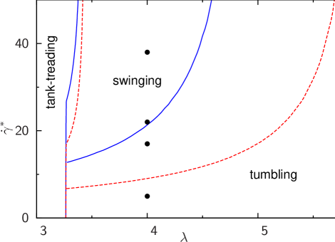
Figure 2: (Color online) Phase diagram at $A^{*}=0.7$. Dashed (red) and solid (blue) lines represent the results of the generalized Keller-Skalak theory with $b_{1}=3/[2(\lambda+1)]$ (see Eq. (5)) and $b_{1}=1/(\lambda+1)$, respectively. The black circles ($\bullet$) indicate the location of the simulation which are shown in Fig. 5.

MPC simulation results of the three dynamical regimes (TT, TB, SW) are illustrated by a sequence of snapshots in Fig. 3. Fig. 3(a) shows a tank-treading vesicle, which has a constant shape and orientation (except for its thermal membrane undulations). However, as a marker on the membrane indicates, the membrane rotates around the center of mass. A tumbling vesicle is shown in Fig. 3(b), where the shape remains almost unchanged, but the orientation steadily rotates. The motion of a marker on the membrane shows that the membrane is not completely fixed with respect to the vesicle shape. Fig. 3(c) illustrates the swinging state (see also movie mov (a)). As long as the vesicle orientation has a positive inclination angle, the elongational part of the shear flow causes an elongation of the vesicle shape (increasing $\alpha$). For a large shape parameter $\alpha$, the vesicle is temporarily in the tumbling regime, until a negative inclination angle $\theta$ is reached (for $0\leq t\dot{\gamma}\leq 10$ in Fig. 3(c)). For negative $\theta$, the elongational component of the flow acts to reduce $\alpha$. Due to the constraint of fixed perimeter $L_{\rm p}$ and fixed enclosed area $A$, the vesicle assumes a potato-like shape, such that $\alpha$ decreases (for $10\leq t\dot{\gamma}\leq 15$ in Fig. 3(c)). The vesicle is then stretched again by the elongational flow leading to a positive inclination angle $\theta$ and increasing shape parameters $\alpha$ (for $t\dot{\gamma}\gtrsim 20$).

It is important to note that elliptical deformations are not sufficient in $2$D, because the constraints on perimeter and area complete determine the elliptical shape Finken et al. (2008) — in contrast to $3$D, where the deformation in the vorticity direction provides sufficient degrees of freedom Noguchi and Gompper (2007). Thus, higher-order undulation modes beyond elliptical deformation are required, which can be seen clearly in Fig. 3(c). This is reminiscent of the behavior of $3$D vesicles in an elongational flow after flow reversal Kantsler et al. (2007); Turitsyn and Vergeles (2008), where also higher-order undulation modes play an important role.

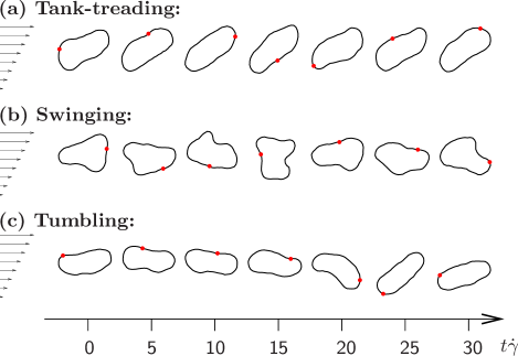
Figure 3: (Color online) Sequences of vesicle snapshots for each of the dynamical regimes, shown (a: TT, b: SW, c: TB). A (red) bullet marks one fixed membrane element to indicate the membrane motion. All systems share the parameters $\kappa/l=50k_{\rm B}T$ and $A^{*}=0.7$. Further parameters are (a) $\eta_{\rm{out}}=36\sqrt{k_{\rm B}Tm}/a$, $\lambda=1$, $\dot{\gamma}=0.01\sqrt{k_{\rm B}T/m}/a$ corresponding to $\dot{\gamma}^{*}=3.6$; (b) $\eta_{\rm{out}}=120\sqrt{k_{\rm B}Tm}/a$, $\lambda=4$, $\dot{\gamma}=0.0333\sqrt{k_{\rm B}T/m}/a$ corresponding to $\dot{\gamma}^{*}=38$; and (c) $\eta_{\rm{out}}=36\sqrt{k_{\rm B}Tm}/a$, $\lambda=10$, $\dot{\gamma}=0.01\sqrt{k_{\rm B}T/m}/a$ corresponding to $\dot{\gamma}^{*}=3.6$.

III.2 TT-TB Transition

The generalized KS theory predicts that for small shear rates, with $\dot{\gamma}^{*}\lesssim 6$, the TT-TB transition at $\lambda\simeq 3.25$ hardly depends on $\dot{\gamma}^{*}$ (see Fig. 2). In this regime, shape deformations are very small, and the behavior can be well described by the original KS theory. We choose a shear rate $\dot{\gamma}=0.01\sqrt{k_{\rm B}T/ma^{2}}$ in our simulation, corresponding to a small reduced shear rate $\dot{\gamma}^{*}=3.6$.

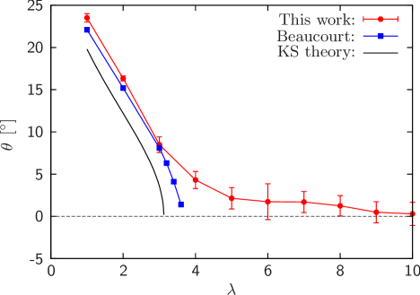
Figure 4: (Color online) Inclination angle $\theta$ as a function of viscosity contrast $\lambda$ for simulations with $\dot{\gamma}^{*}=3.6$. For comparison the results of the boundary-integral calculation of Beaucourt et al. Beaucourt et al. (2004) (without thermal fluctuations) as well as the curve of KS theory Keller and Skalak (1982) (see Eq. (30)) are shown.

In Fig. 4, the dependence of the average inclination angle $\theta$ on the viscosity contrast $\lambda$ is shown. Our MPC simulations well reproduce the results of previous boundary-integral calculations by Beaucourt et al. Beaucourt et al. (2004). Deviations close to the TT-TB transition at $\lambda^{*}\simeq 4$ arise from thermal membrane undulations, which are present in our simulations, whereas the results of Ref. Beaucourt et al. (2004) have been obtained in the zero-temperature limit.

Moreover, thermal fluctuations lead to a continuous crossover rather than a sharp TT-TB transition. Thus, there are a few tumbling events already for viscosity contrast $\lambda=3$, and also simulations with $\lambda>\lambda^{*}\simeq 4$ exhibit some time intervals of tank-treading motion. Our simulations also show that the existence of a tumbling regime depends sensitively on the Reynolds number Re. For Re $\gtrsim 1$, $\theta$ decreases more gradually with increasing $\lambda$, and no tumbling motion was observed at viscosity contrasts as large as $\lambda=10$. Thus, we conclude that inertial effects enhance the TT-membrane rotation.

Fig. 4 also shows that KS theory Keller and Skalak (1982) provides a good description of the $\lambda$ dependence of $\theta$ and the TT-TB transition. This transition is explained by the KS theory as follows. The stationary inclination angle $\theta$ in the tank-treading regime is determined by Eq. (4) with fixed $\alpha$ as

$$\theta=-\frac{1}{2}\arccos\left(-\frac{1}{B}\right).$$ (30)

For small $\lambda$, the inclination angle $\theta$ decreases monotonically up to a critical viscosity contrast $\lambda^{*}$, where $\theta=0$. For larger viscosity contrasts $\lambda>\lambda^{*}$, the tumbling regime, there is no real solution of Eq. (30), i.e. no stationary inclination angle exists, and the vesicle permanently rotates.

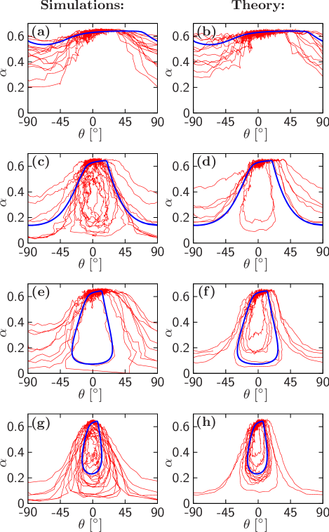
Figure 5: (Color online) Trajectories in the $\theta$-$\alpha$ plane for $\lambda=4$, both with (thin red lines) and without (thick blue lines) thermal noise. The trajectories in (a), (c), (d), and (g) are obtained from simulations, whereas the curves in (b), (d), (f), and (h) are calculated from the generalized KS theory with noise and $b_{1}=1/(\lambda+1)$. The reduced shear rates are $\dot{\gamma}^{*}=5$ for (a) and (b), $\dot{\gamma}^{*}=17$ for (c) and (d), $\dot{\gamma}^{*}=22$ for (e) and (f), and $\dot{\gamma}^{*}=38$ for (g) and (h). In all plots, the corresponding theoretical trajectory according the generalized Keller-Skalak theory without thermal noise is shown as a thick blue (dark) line.

III.3 TB-SW Transition

To investigate the TB-SW transition, we consider a fixed viscosity contrast of $\lambda=4$, and perform simulations for four different reduced shear rates $\dot{\gamma}^{*}=5,17,22$, and $38$. The locations of these four shear rates in the dynamical phase diagram are indicated in Fig. 2. The resulting trajectories in the $\theta$-$\alpha$ plane are shown on the left-hand side of Fig. 5. In this representation, closed cycles indicate swinging events, whereas trajectories spanning the full $[-\pi/2,+\pi/2]$ range of $\theta$ are tumbling events. Obviously, thermal noise has a large impact on the vesicle dynamics. In particular, at small inclination angles $\theta\simeq 0$, small thermal fluctuations are decisive for the vesicle to perform a tumbling or swinging cycle.

The simulation data of Fig. 5 suggest that the TB-SW transition point is located between $\dot{\gamma}^{*}=17$ and $22$. This is about a factor $2$ larger than the prediction $\dot{\gamma}^{*}=9$ of generalized KS theory. In the generalized KS theory, a possible source of error can be found in the estimate of $b_{0}$ and $b_{1}$, which have both been calculated in the circular limit, see Eq. (5). Therefore, we also calculate the phase diagram with $b_{1}$ reduced by a factor $2/3$, i.e. with $b_{1}=1/(\lambda+1)$, which gives a better agreement with our simulations for non-circular vesicles with $A^{*}=0.7$ (see Fig. 2). In this case, the effect of thermal noise on trajectories is found to be very similar as in the simulations for all four reduced shear rates (see Fig. 5). Therefore, the deviations between the generalized KS theory and simulations can be alleviated by a small modification of prefactors. Further theoretical developments are needed to determine the prefactors $b_{0}$ and $b_{1}$ analytically for non-circular shapes. We conclude that generalized KS theory provides a good description of vesicle dynamics in shear flow in both two and three spatial dimensions.

Elastic capsules Chang and Olbricht (1993); Navot (1998) and red blood cells Abkarian et al. (2007) can also exhibit a swinging motion. However, the angle $\theta(t)$ is always positive during these oscillations — unlike SW of fluid vesicles. The physical mechanism is an energy barrier for the TT rotation caused by the membrane shear elasticity and the anisotropic shape of the spectrin network Abkarian et al. (2007); Skotheim and Secomb (2007); Kessler et al. (2008). Although, a vesicle in $2$D (a closed string) does not have membrane shear elasticity, an energy barrier for the TT rotation can be introduced by inhomogeneities in the spontaneous curvature Sui et al. (2007). In the future, it will be interesting to investigate the coupling of different swinging mechanisms in composite membranes.

IV Lift Force

We now consider a vesicle under the combined effect of a shear flow and a gravitational force $F_{\rm G}$, see Fig. 6(a). The vesicle moves towards or away from the wall until gravitational $F_{\rm G}$ and lift forces $F_{\rm L}(y_{\rm{cm}})$ balance each other (see also movie mov (b)). In this steady state, the lift force $F_{\rm L}(y_{\rm cm})$ equals the gravitational force in magnitude.

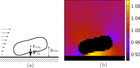
Figure 6: (Color) (a) Shape and (b) pressure field of a tank-treading vesicle under shear flow close to a wall, in steady state with viscosity contrast $\lambda=3$. The color code is expressed in units of $n_{\rm s}k_{\rm B}T$. The hydrodynamic lift force is balanced by an external gravitational force $F_{\rm G}=14k_{\rm B}T/a$, where the average distance from the wall is $y_{\rm{cm}}=7.96a$. See also movie mov (b).

Fig. 6(b) shows the pressure field in the outer fluid for the steady-state configuration of a tank-treading vesicle. The hydrodynamic lift force is the integral of the pressure forces over the membrane contour. The higher pressure in the gap between the vesicle and the wall is responsible for the lift force. Fig. 6(b) also nicely demonstrates that there is a lower pressure at the two caps of the vesicle, which is the origin of vesicle elongation. The hydrodynamic lift force is a pressure force which is of purely viscous nature – in contrast to e.g. aerodynamic forces acting on the wings of an airplane, which are caused by inertial forces.

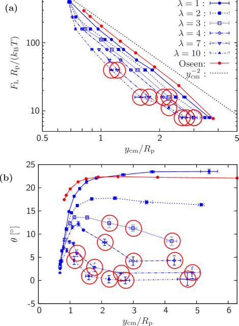
Figure 7: (Color online) (a) Lift forces and (b) average inclination angle as a function of the average wall distance $y_{\rm{cm}}$ of the vesicle, from MPC simulations with $\dot{\gamma}^{*}=3.6$ and from boundary-integral (Oseen) calculations, as indicated. The legend in (a) applies to both plots. Simulation points marked by big (red) circles refer to tumbling vesicles. For comparison, a line with the power-law dependence $y^{-2}_{\rm{cm}}$ is plotted in (a). The right-most data points in (b) correspond to $F_{\rm G}=0$, so that they cannot be shown in the double-logarithmic presentation in (a).

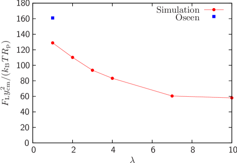
Figure 8: (Color online) Amplitude of the lift force, $F_{\rm L}y_{\rm cm}^{2}/(k_{\rm B}TR_{\rm p})$, as a function of the viscosity contrast $\lambda$. The amplitudes are fits to the curves in Fig. 7(a) for which vesicles are not in direct contact with the wall.

The dependence of the hydrodynamic lift force on the wall distance is shown in Fig. 7(a) — calculated as $\langle y_{\rm cm}\rangle$ for fixed gravitational force in the simulations, and as lift force at fixed $y_{\rm cm}$ in the Oseen calculations, as explained in detail in Sec. II.3.3 and Sec. II.4 above. Lift forces of vesicles with $\lambda\leq 4$ can be well described by a power-law $F_{\rm L}\propto y^{-2}_{\rm{cm}}$ for $F_{\rm L}\leq 2.5k_{\rm B}T/R_{\rm p}$, corresponding to $y_{\rm{cm}}\gtrsim R_{\rm p}$. For these distances, the vesicle is not in direct contact with the wall. At applied gravitational forces larger than $2.5k_{\rm B}T/R_{\rm p}$, the vesicle touches the wall ($y_{\rm{cm}}\lesssim R_{\rm p}$). However, the distance $y_{\rm{cm}}$ between the center of mass and the wall can be reduced even further by vesicle deformation. The $1/y^{2}_{\rm{cm}}$ dependence does not apply in this regime. Finally, the constraints of fixed enclosed area $A$ and fixed perimeter $L_{\rm p}$ keep the wall distance larger than $y_{\rm{cm}}\gtrsim 0.628R_{\rm p}$.

Fig. 7(a) shows that the lift forces decrease with increasing viscosity ratio $\lambda$ for a fixed wall distance $y_{\rm{cm}}$. This behavior is analyzed in more detail in Fig. 8, where the amplitude $F_{\rm L}y^{2}_{\rm{cm}}$ of the lift force is plotted as a function of the viscosity contrast $\lambda$. Although solid colloidal particles of elliptical shape experience no net lift force Pozrikidis (2006), tumbling vesicles with finite $\lambda$ obtain lift force due to an asymmetry of its shape deformations and a small tank-treading component (compare Fig. 3(c)).

For vesicles in three dimensions, both boundary-integral simulations Sukumaran and Seifert (2001) as well as theoretical studies Olla (1997a, b) show a $1/y^{2}_{\rm{cm}}$ dependence of the lift force for vesicles far from the wall. The theory of Olla Olla (1997a, b) assumes an ellipsoidal shape for the vesicles with half axes $a_{1},a_{2},a_{3}\ll y_{\rm{cm}}$. It is not possible in this case to derive expressions for two dimensions by taking the limit $a_{3}\to\infty$ — as done in App. A for KS theory of vesicles in unbounded flows — because this limit is inconsistent with the assumption $a_{1},a_{2},a_{3}\ll y_{\rm{cm}}$. Therefore, instead of an analytical theory, we perform boundary-integral calculations of $2$D elliptical vesicles with $\lambda=1$ in the presence of a wall, as described in Sec. II.4. For the results in Fig. 7(a), the effect of the opposite wall at $L_{y}=10R_{\rm p}$ is also taken into account by plotting $F_{\rm L}(y_{\rm{cm}})-F_{\rm L}(L_{y}-y_{\rm{cm}})$, where $F_{\rm L}(y_{\rm{cm}})$ and $F_{\rm L}(L_{y}-y_{\rm{cm}})$ are obtained from two independent boundary-integral calculations. Of course, a more precise calculation would require the use the two-wall Oseen tensor Pozrikidis (1992) instead of the half-space Greens function. However, as long as the distance $L_{y}$ between the two walls is sufficiently large, $F_{\rm L}(y_{\rm{cm}})-F_{\rm L}(L_{y}-y_{\rm{cm}})$ is a good approximation of the two-wall lift force. Fig. 7(a) as well as Fig. 8 show that the boundary-integral calculation indeed agrees nicely with the corresponding MPC simulation for $\lambda=1$. The amplitudes $F_{\rm L}{y_{\rm{cm}}}^{2}$ only differ by about 25%. Reasons for this deviation are that the boundary-integral calculation is done for elliptical shapes, whereas vesicles in simulations are closer to the equilibrium shape (compare Fig. 1 and Fig. 6). Moreover thermal fluctuations in the MPC simulations may cause differences.

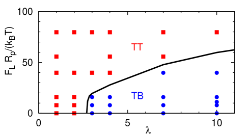
Figure 9: (Color online) Dynamic phase diagram of tank-treading and tumbling states as a function of the gravitational force $F_{\rm G}$ and the viscosity contrast $\lambda$. The reduced shear rate is $\dot{\gamma}^{*}=3.6$. Circles ($\bullet$) indicate tumbling motion (TB), squares ($\blacksquare$) tank-treading motion (TT). The line for the phase boundary is a guide to the eye.

Fig. 7(a) shows that tumbling is suppressed when the gravitational force exceeds a threshold value, depending on the viscosity contrast $\lambda$. In order to perform a tumbling motion, the center-of-mass distance $y_{\rm{cm}}$ has to be on the order of or larger than the long vesicle axis $a_{1}$. However, for larger gravitational forces, the center-of-mass distance $y_{\rm{cm}}$ becomes smaller than $a_{1}$, such that even vesicles with high viscosity contrasts do not tumble. Even if $y_{\rm{cm}}$ is slightly larger than $a_{1}$, the vesicle cap has to come so close to the wall that the resulting pressure forces prevent the inclination angle to reach $\pi/2$. This leads to the dynamical phase diagram shown in Fig. 9. When the gravitational force is large, tumbling is suppressed and the vesicle displays a tank-treading motion at the wall. With increasing $\lambda$, the gravitational force necessary to prevent tumbling increases.

The dependence of the inclination angle $\theta$ on the wall distance $y_{\rm{cm}}$ is shown in Fig. 7(b). Without a gravitational force, the lift force caused by the upper wall at $y=10R_{\rm p}$ compensates the lift force of the lower wall when the vesicle is in the center, at $y_{\rm{cm}}=5R_{\rm p}$. Since the lift forces are very small nearby, strong fluctuations are observed in the wall distances for small $F_{\rm G}$.

As long as a vesicle is tank-treading, its inclination angle $\theta$ decreases when it approaches the wall. Even if the vesicle does not touch the wall, the pressure at the lowest part of the membrane is highest (see Fig. 6(b)) such that it causes a torque which lowers $\theta$. For very small wall distances, the vesicle comes into direct contact with the wall, where the repulsive wall potential causes an additional torque, which decreases $\theta$ even further, until the vesicle is finally completely parallel to the wall.

Vesicles with $\lambda\geq 3$ start to tumble at sufficiently large wall distances. Since vesicles with viscosity ratios $\lambda=3$ and $\lambda=4$ are still tank-treading most of the time and only occasionally perform a tumbling motion, their inclination angles are non-zero, whereas for $\lambda=10$ and $F_{\rm G}\leq 1$, the average inclination angle $\theta$ essentially vanishes (see Fig. 7(b)).

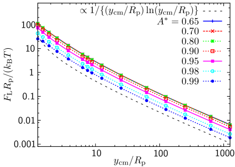
Figure 10: (Color online) Hydrodynamic lift force $F_{\rm L}$ on vesicles with varying $A^{*}$ vs. wall distance $y_{\rm{cm}}$ obtained from boundary-integral calculations.

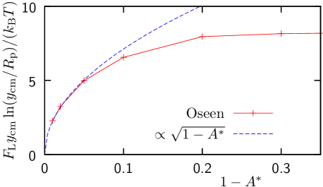
Figure 11: (Color online) Amplitude of the lift force $F_{\rm L}$ as a function of $1-A^{*}$. The data points are fits to the curves in Fig. 10 for $y_{\rm{cm}}\geq 60R_{\rm p}$. These data points (Oseen) are fitted to a $\sqrt{1-A^{*}}$ dependence for small values of $1-A^{*}$.

We employ the boundary-integral approach to calculate the dependence of the hydrodynamic lift force of vesicles with $\lambda=1$ on the reduced area $A^{*}$ in the absence of thermal fluctuations. Also, since this method is not restricted by the system size (as simulations), the lift forces can be calculated even for very large wall distances. Fig. 10 shows the hydrodynamic lift force as a function of the wall distance $y_{\rm{cm}}$ for different reduced areas $A^{*}$ in the range $0.65\leq A^{*}\leq 0.99$. This plot shows that the $y_{\rm{cm}}^{-2}$ dependence of the hydrodynamic lift force $F_{\rm L}$ only holds for distances $y_{\rm{cm}}\lesssim 5R_{\rm p}$ from the wall. For larger distances $y_{\rm{cm}}$, a crossover to a $1/\left[(y_{\rm{cm}}/R_{\rm p})\ln\left(y_{\rm{cm}}/R_{\rm p}\right)\right]$ dependence is obtained. This power law with a logarithmic correction fits perfectly the numerical data of the boundary-integral calculation for $y_{\rm cm}\gtrsim 2R_{\rm p}$ for all considered reduced areas. Fig. 11 shows the amplitudes $K=F_{\rm L}y_{\rm{cm}}\ln(y_{\rm{cm}}/R_{\rm p})$ of the lift forces $F_{\rm L}$ vs. $1-A^{*}$ in the far-field limit. These amplitudes $K$ are determined by fitting the expression $F_{\rm L}=K/\left[(y_{\rm{cm}}/R_{\rm p})\ln\left(y_{\rm{cm}}/R_{\rm p}\right)\right]$ to all data with $y_{\rm{cm}}\geq 60R_{\rm p}$. For $1-A^{*}=0$, i.e. for a circular vesicle, the lift force vanishes, which directly follows from the time-inversion symmetry of the Stokes equation. For small deviations from the circular shape, the lift force rapidly increases with $1-A^{*}$, and follows a power-law dependence $K\sim\sqrt{1-A^{*}}$ $\simeq\sqrt{\Delta_{\rm p}/\pi}$, with the excess length $\Delta_{\rm p}=L_{\rm p}/R_{\rm A}-2\pi$, for $1-A^{*}\lesssim 0.1$ (see Fig. 11). We observe a monotonic increase of the lift force with increasing $1-A^{*}$ over the whole range of reduced areas $A^{*}$.

Since boundary-integral calculations do not take into account thermal fluctuations, lift forces can be determined for large $y_{\rm{cm}}$ (only limited by numerical accuracy). However in simulations as well as in real systems, lift forces at large $y_{\rm{cm}}$ have a vanishing effect compared to thermal noise. Moreover, with very large wall distance $y_{\rm{cm}}\sim\sqrt{\eta_{\rm{out}}/\rho\dot{\gamma}}$, inertial effects are not negligible, so that the Stokes approximation becomes less reliable Olla (1997b).

V Summary and Conclusion

We have studied the dynamics of vesicles in shear flow in a two-dimensional model system. This system shows a variety of interesting dynamical phenomena.

First, we have investigated the effect of the viscosity contrast $\lambda$, i.e. the ratio between the inner and outer viscosities of a vesicle, on the dynamics in unbounded flows. With increasing $\lambda$, the sequence from “tank-treading” over “swinging” to “tumbling” motion is generically observed — except for small shear rates $\dot{\gamma}$, where the intermediate swinging phase is absent. Thus, the swinging phase appears in the phase diagram of $2$D vesicles under shear in the same way as it was found previously for $3$D ellipsoidal vesicles. However, the mechanism of swinging is different in two and three dimensions. While in $3$D, ellipsoidal deformations are sufficient to obtain swinging, in $2$D higher-order undulation modes are required. Thermal fluctuations play an important role; they lead to a smooth crossover between the dynamical states, with intermittent tumbling and tank-treading motions. Our simulations are in semi-quantitative agreement with a theoretical description based on a generalized Keller-Skalak approach.

Second, we have investigated the behavior of vesicles near walls. Close to a wall, tumbling is strongly suppressed. Furthermore, the vesicle is repelled from the wall by the hydrodynamical lift force. We have found by boundary-integral calculations that the hydrodynamic lift force decays with increasing wall distance $y_{\rm{cm}}$ like $1/\left(y_{\rm{cm}}\ln y_{\rm{cm}}\right)$. However, for small wall distances – in particular in the regime of the MPC simulations – an effective $y_{\rm{cm}}^{-2}$ dependence is observed. With increasing viscosity contrast, the lift force becomes weaker, as the vesicle becomes less deformable. The lift force also decreases with increasing reduced area $A^{*}$, and vanishes in the circular limit. We find that our numerical data are well described by a $\sqrt{1-A^{*}}$ dependence.

Our results show that there is a different behavior of the lift force at intermediate and large distances from the wall, and that the lift force decreases significantly with increasing viscosity contrast. This may shed some light on the behavior in three dimensions, where experiments show a dependence of the lift force on the wall-membrane distance $h$, which decays as $h^{-1}$ for distances smaller than the vesicle radius Abkarian et al. (2002), whereas a $y_{\rm cm}^{-2}$ decay has been found theoretically in a small range $1.1\lesssim y_{\rm cm}/R_{\rm p}\lesssim 1.25$ of wall distances Sukumaran and Seifert (2001). Thus, we hope that our results will stimulate new experiments and simulations in $3$D over a wider range of wall distances, reduced volumes, and viscosity contrasts.

Appendix A Derivation of 2D Generalized Keller-Skalak Theory

A.1 Keller-Skalak Theory in Two Dimensions

Keller and Skalak Keller and Skalak (1982) derived analytical expressions for the inclination angle $\theta$ and the average angular velocity $\omega$ for $3$D vesicles of fixed ellipsoidal shape, with $(x/a_{1})^{2}+(y/a_{2})^{2}+(z/a_{3})^{2}=1$, based on the Jeffery theory Jeffery (1922).

Although the KS theory is formulated for vesicles in three dimensions, it is straightforward to transfer it to two-dimensional systems by simply taking the limit $a_{3}\to\infty$. The resulting cylindrical three-dimensional geometry is equivalent to a $2$D vesicle with the shape of an ellipse, $(x/a_{1})^{2}+(y/a_{2})^{2}=1$ with $a_{1}\geq a_{2}$. Let $S^{\prime}$ be the frame which has its origin at the center of the ellipse, and the $x^{\prime}$ direction points into the direction of the long axis. Then the local velocity ${\bf v}^{\prime}$ of an element of the tank-treading membrane is assumed to be

$$(v_{x}^{\prime},v_{y}^{\prime})=\omega(-\frac{a_{1}}{a_{2}}x_{2}^{\prime},\frac{a_{2}}{a_{1}}x_{1}^{\prime}).$$ (31)

in the frame $S^{\prime}$. We define the auxiliary variables

$$f_{0}:=\frac{1-{\alpha_{\rm D}}^{2}}{1+{\alpha_{\rm D}}^{2}},\qquad f_{1}:=\frac{1-{\alpha_{\rm D}}^{2}}{8\alpha_{\rm D}},\qquad f_{2}:=\frac{1+{\alpha_{\rm D}}^{2}}{2},$$

where $\alpha_{\rm D}=(a_{1}+a_{2})/(a_{1}-a_{2})$. The balance of torques on the membrane and the assumption that the work done on the vesicles by the shear flow is dissipated in the interior of the vesicle leads to the non-linear differential equation

$$\frac{d\theta}{dt} = \frac{\dot{\gamma}}{2}\left[-1+B(\alpha_{\rm D},\lambda)\cos(2\theta)\right]$$ (32)

$$B(\alpha_{\rm D},\lambda) = f_{0}\left\{f_{1}+\frac{f_{1}^{-1}}{1+f_{2}(\lambda-1)}\right\}.$$ (33)

Furthermore, the average angular velocity $\omega$ is found to be

$$\frac{\omega}{\dot{\gamma}}=\frac{\cos(2\theta)}{2f_{1}\{1+f_{2}(\lambda-1)\}}$$ (34)

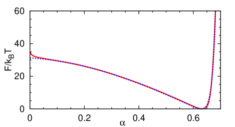
Figure 12: (Color online) Free energy $F(\alpha)$ of the two-dimensional vesicle relative to the prolate shape for $A^{*}=0.7$, $\kappa/l=50k_{\rm B}T$, $k_{\rm{sp}}=10^{4}k_{\rm B}T/a^{2}$, and $k_{\rm A}=80k_{\rm B}T/a^{4}$. The solid (red) and dashed (blue) lines represent the simulation data and fitted curve, respectively.

A.2 Shape Equation in Two Dimensions

The vesicle shape is expanded in Fourier modes with polar angle $\phi$ as ${\bf r}(\phi)=R_{\rm A}{\bf e}_{r}\{1+\sum u_{m}\exp(im\phi/\sqrt{2\pi})\}$. Based on the Stokes approximation and perturbation theory, the dynamics of a quasi-circular vesicle is described by Finken et al. (2008)

$$\frac{\partial u_{m}}{\partial t}=\frac{i\dot{\gamma}m}{2}u_{m}-\frac{\kappa\Gamma_{m}E_{m}}{\eta_{\rm{out}}R_{\rm A}^{3}}{u_{m}}\mp ih\dot{\gamma}\delta_{m,\pm 2},$$ (35)

where $\Gamma_{m}=|m|/2(\lambda+1)(m^{2}-1)$, $E_{m}=(m^{2}-1)(m^{2}-3/2+\sigma)$, and $h=\sqrt{2\pi}/2(\lambda+1)$. A Lagrange multiplier $\sigma$ keeps the perimeter $L_{\rm p}$ constant. Following the procedure for $3$D Noguchi and Gompper (2007), we decompose $u_{\pm 2}$ into amplitude and phase, $u_{\pm 2}=r\exp(\mp 2i\theta)$, and replace the force $2\kappa E_{m}r$ by $\partial F/\partial r$. Then, Eq. (3) is obtained with $\alpha=3r/\sqrt{2\pi}+O(r^{2})$.

The free energy $F(\alpha)$ for the same simulation parameters calculated with a version of the generalized-ensemble Monte Carlo method Noguchi and Gompper (2005) (see Fig. 12): The vesicle conformations are sampled under the uniform distribution of $\alpha$, and then the canonical distribution is obtained by the reweighing. Instead of an interpolation Noguchi and Gompper (2004, 2005, 2007), we use fit functions here to obtain smooth functions. The force is fitted as a function $-(1/k_{\rm B}T)\partial F/\partial\alpha=9+180\alpha-110\alpha^{2}-\exp(80\alpha-46)$. We obtained the relation $\alpha_{\rm D}=2\alpha/3+0.14\alpha^{4}$ by fitting for the ellipse of $A^{*}=0.7$.

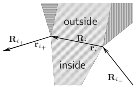
Figure 13: Spatial regions for the membrane collision between MPC particles and membrane monomers. MPC particles located in the dark-gray regions perform a two-body collision with the monomers $i$ or $i_{+}$. MPC particles in the light-gray regions collide with both monomers. For further explanations, see text.

Appendix B Membrane Collisions with the Solvent

For the modeling of an impermeable membrane, interior and exterior solvent particles have to stay on the appropriate side of the membrane. Depending on the position of the MPC particle with respect to membrane bonds, either one or two membrane monomers participate in a membrane collision. The new velocities of the $n_{\rm{coll}}$ particles (the MPC particle and the $n_{\rm{coll}}-1$ membrane monomers) after the collision are then

$${\bf v}_{i,{\rm{new}}}=2\left({\bf v}_{\rm{cm}}+{\bf\omega}\times{\bf r}_{i,c}\right)-{\bf v}_{i},$$ (36)

where $v_{\rm{cm}}$ is the center-of-mass velocity of the $n_{\rm{coll}}$-body system, $\omega$ its angular velocity, and ${\bf r}_{i,c}$ are the particle positions relative to the center of mass of the $n_{\rm{coll}}$-body system. This is a bounce-back collision for the relative velocities which conserves both the total translational and angular momenta. The spatial regions for the selection of colliding MPC particles and membrane monomers are illustrated in Fig. 13.

References

- Seifert (1997) U. Seifert, Adv. Phys. 46, 13 (1997).
- Keller and Skalak (1982) S. R. Keller and R. Skalak, J. Fluid Mech. 120, 27 (1982).
- Kraus et al. (1996) M. Kraus, W. Wintz, U. Seifert, and R. Lipowsky, Phys. Rev. Lett. 77, 3685 (1996).
- Beaucourt et al. (2004) J. Beaucourt, F. Rioual, T. Seon, T. Biben, and C. Misbah, Phys. Rev. E 69, 011906 (2004).
- Noguchi and Gompper (2004) H. Noguchi and G. Gompper, Phys. Rev. Lett. 93, 258102 (2004).
- Noguchi and Gompper (2005) H. Noguchi and G. Gompper, Phys. Rev. E 72, 011901 (2005).
- Noguchi (2009) H. Noguchi, J. Phys. Soc. Jpn. 78, 041007 (2009).
- Pozrikidis (2001) C. Pozrikidis, J. Fluid Mech. 440, 269 (2001).
- de Haas et al. (1997) K. H. de Haas, C. Blom, D. van den Ende, M. H. G. Duits, and J. Mellema, Phys. Rev. E 56, 7132 (1997).
- Kantsler and Steinberg (2005) V. Kantsler and V. Steinberg, Phys. Rev. Lett. 95, 258101 (2005).
- Kantsler and Steinberg (2006) V. Kantsler and V. Steinberg, Phys. Rev. Lett. 96, 036001 (2006).
- Mader et al. (2006) M. A. Mader, V. Vitkova, M. Abkarian, A. Viallat, and T. Podgorski, Eur. Phys. J. E 19, 389 (2006).
- Misbah (2006) C. Misbah, Phys. Rev. Lett. 96, 028104 (2006).
- Vlahovska and Gracia (2007) P. M. Vlahovska and R. S. Gracia, Phys. Rev. E 75, 016313 (2007).
- Noguchi and Gompper (2007) H. Noguchi and G. Gompper, Phys. Rev. Lett. 98, 128103 (2007).
- Danker et al. (2007) G. Danker, T. Biben, T. Podgorski, C. Verdier, and C. Misbah, Phys. Rev. E 76, 041905 (2007).
- Lebedev et al. (2007) V. V. Lebedev, K. S. Turitsyn, and S. S. Vergeles, Phys. Rev. Lett. 99, 218101 (2007).
- Lebedev et al. (2008) V. V. Lebedev, K. S. Turitsyn, and S. S. Vergeles, New. J. Phys. 10, 043044 (2008).
- Fung (1997) Y. C. Fung, Biomechanics: circulation (Springer, New York, 1997), 2nd ed.
- Imhof and Dunon (1997) B. A. Imhof and D. Dunon, Hormone And Metabolic Research 29, 614 (1997).
- Chang et al. (2000) K. C. Chang, D. F. J. Tees, and D. A. Hammer, Proc. Natl. Acad. Sci. USA 97, 11262 (2000).
- Dwir et al. (2003) O. Dwir, A. Solomon, S. Mangan, G. S. Kansas, U. S. Schwarz, and R. Alon, J. Cell Biol. 163, 649 (2003).
- Poiseuille (1836) J. L. M. Poiseuille, Ann. Sci. Nat. 5, 111 (1836).
- Olla (1997a) P. Olla, J. Phys. II 7, 1533 (1997a).
- Olla (1997b) P. Olla, J. Phys. A: Math. Gen. 30, 317 (1997b).
- Cantat and Misbah (1999) I. Cantat and C. Misbah, Phys. Rev. Lett. 83, 880 (1999).
- Seifert (1999) U. Seifert, Phys. Rev. Lett. 83, 876 (1999).
- Sukumaran and Seifert (2001) S. Sukumaran and U. Seifert, Phys. Rev. E 64, 011916 (2001).
- Lorz et al. (2000) B. Lorz, R. Simson, J. Nardi, and E. Sackmann, Europhys. Lett. 51, 468 (2000).
- Abkarian et al. (2002) M. Abkarian, C. Lartigue, and A. Viallat, Phys. Rev. Lett. 88, 068103 (2002).
- Abkarian and Viallat (2005) M. Abkarian and A. Viallat, Biophys. J. 89, 1055 (2005).
- Callens et al. (2008) N. Callens, C. Minetti, G. Coupier, M. A. Mader, F. Dubois, C. Misbah, and T. Podgorski, EPL 83, 24002 (2008).
- Finken et al. (2008) R. Finken, A. Lamura, U. Seifert, and G. Gompper, Eur. Phys. J. E 25, 309 (2008).
- Malevanets and Kapral (1999) A. Malevanets and R. Kapral, J. Chem. Phys. 110, 8605 (1999).
- Kapral (2008) R. Kapral, Adv. Chem. Phys. 140, 89 (2008).
- Gompper et al. (2009) G. Gompper, T. Ihle, D. M. Kroll, and R. G. Winkler, Adv. Polym. Sci. 221, 1 (2009).
- Noguchi et al. (2007) H. Noguchi, N. Kikuchi, and G. Gompper, EPL 78, 10005 (2007).
- Noguchi and Gompper (2008) H. Noguchi and G. Gompper, Phys. Rev. E 78, 016706 (2008).
- Götze et al. (2007) I. O. Götze, H. Noguchi, and G. Gompper, Phys. Rev. E 76, 046705 (2007).
- Pozrikidis (1992) C. Pozrikidis, Boundary integral and singularity methods for linearized viscous flow (Cambridge University Press, Cambridge, 1992).
- mov (a) See EPAPS Document No. [number will be inserted by publisher] for movies of the dynamics of a vesicle in unbounded shear flow in the swinging regime. For more information on EPAPS, see http://www.aip.org/pubservs/epaps.html.
- Kantsler et al. (2007) V. Kantsler, E. Segre, and V. Steinberg, Phys. Rev. Lett. 99, 178102 (2007).
- Turitsyn and Vergeles (2008) K. S. Turitsyn and S. S. Vergeles, Phys. Rev. Lett. 100, 028103 (2008).
- Chang and Olbricht (1993) K. S. Chang and W. L. Olbricht, J. Fluid Mech. 250, 609 (1993).
- Navot (1998) Y. Navot, Phys. Fluids 10, 1819 (1998).
- Abkarian et al. (2007) M. Abkarian, M. Faivre, and A. Viallat, Phys. Rev. Lett. 98, 188302 (2007).
- Skotheim and Secomb (2007) J. M. Skotheim and T. W. Secomb, Phys. Rev. Lett. 98, 078301 (2007).
- Kessler et al. (2008) S. Kessler, R. Finken, and U. Seifert, J. Fluid Mech. 605, 207 (2008).
- Sui et al. (2007) Y. Sui, Y. T. Chew, P. Roy, X. B. Chen, and H. T. Low, Phys. Rev. E 75, 066301 (2007).
- mov (b) See EPAPS Document No. [number will be inserted by publisher] for movies of the dynamics of a vesicle near a wall under the effect of a gravitational force. For more information on EPAPS, see http://www.aip.org/pubservs/epaps.html.
- Pozrikidis (2006) C. Pozrikidis, J. Fluid Mech. 568, 161 (2006).
- Jeffery (1922) G. B. Jeffery, Proc. R. Soc. London Ser. A 102, 161 (1922).