Finite-size effects at first-order isotropic-to-nematic transitions

Abstract

We present simulation data of first-order isotropic-to-nematic transitions in lattice models of liquid crystals and locate the thermodynamic limit inverse transition temperature $\epsilon_{\infty}$ via finite-size scaling. We observe that the inverse temperature of the specific heat maximum can be consistently extrapolated to $\epsilon_{\infty}$ assuming the usual $\alpha/L^{d}$ dependence, with $L$ the system size, $d$ the lattice dimension and proportionality constant $\alpha$. We also investigate the quantity $\epsilon_{L,k}$, the finite-size inverse temperature where $k$ is the ratio of weights of the isotropic to nematic phase. For an optimal value $k=k_{\rm opt}$, $\epsilon_{L,k}$ versus $L$ converges to $\epsilon_{\infty}$ much faster than $\alpha/L^{d}$, providing an economic alternative to locate the transition. Moreover, we find that $\alpha\sim\ln k_{\rm opt}/{\cal L}_{\infty}$, with ${\cal L}_{\infty}$ the latent heat density. This suggests that liquid crystals at first-order IN transitions scale approximately as $q$-state Potts models with $q\sim k_{\rm opt}$.

I Introduction

The investigation of the isotropic-to-nematic (IN) transition in liquid crystals via computer simulation is long established. Decades ago Lebwohl and Lasher (LL) introduced a simple lattice model, the LL model, to study this transition physreva.6.426 . At each site $i$ of a cubic lattice they attached a three-dimensional unit vector $\vec{d}_{i}$ (spin) interacting with its nearest-neighbors via

$${\cal H}=-\epsilon\sum_{<ij>}|\vec{d}_{i}\cdot\vec{d}_{j}|^{p},$$ (1)

where $p=2$ and with a factor $1/k_{B}T$ absorbed into the coupling constant $\epsilon>0$, with $k_{B}$ the Boltzmann constant and $T$ the temperature. Despite its simplicity, the LL model captures certain aspects of liquid crystal phase behaviour remarkably well, and has consequently received considerable attention citeulike:4197190 ; citeulike:4197214 .

A common problem in locating the IN transition via simulation is the issue of finite system size. Phase transitions are defined in the thermodynamic limit, whereas simulations always deal with finite particle numbers. In order to estimate the thermodynamic limit transition point, it is typical to perform a number of simulations for different system sizes and to subsequently extrapolate the results following some finite-size scaling (FSS) procedure. Which procedure to use depends on the type of transition, i.e. whether it is continuous or first-order. In three spatial dimensions, the IN transition is typically first-order; in two dimensions both continuous bates.frenkel:2000 ; physreva.31.1776 ; citeulike:3740617 and first-order vink:2006*b ; vink.wensink:2007 IN transitions can occur, depending on the details of the interactions physrevlett.52.1535 ; physrevlett.89.285702 ; enter.romano.ea:2006 . In this paper we focus on the first-order case.

The literature on FSS at first-order transitions is quite extensive, for a review see citeulike:1920630 , the majority of which deals exclusively with the Potts model note1 . An important result is that the “apparent” transition inverse temperature $\epsilon_{L,CV}$, obtained in a finite system of size $L$, is shifted from the thermodynamic limit value $\epsilon_{\infty}$ as citeulike:3716330 ; citeulike:3720308

$$\epsilon_{L,CV}=\epsilon_{\infty}-\alpha/L^{d}+{\cal O}(1/L^{2d}),$$ (2)

with proportionality constant $\alpha>0$. Here $\epsilon_{L,CV}$ is the inverse temperature where the specific heat in a finite system of size $L$ attains its maximum, $d$ is the spatial dimension of the lattice and $L$ denotes the linear extension of the simulation box, generally square or cubic, with periodic boundary conditions.

We emphasize that Eq.(2) was derived for the Potts model where the proportionality constant is known to be

$$\alpha_{\rm Potts}=\ln q/{\cal L}_{\infty},$$ (3)

with $q$ the number of Potts states and ${\cal L}_{\infty}$ the latent heat density in the thermodynamic limit citeulike:3716330 ; citeulike:3720308 . Interestingly, simulations of the LL model have shown that the functional form of Eq.(2) also works well for IN transitions physrevlett.69.2803 ; citeulike:3740162 . That is, meaningful extrapolations of $\epsilon_{L,CV}$ can be performed, although the significance of $\alpha$ is not obvious. It certainly cannot be related to the number of spin states, i.e. conform to Eq.(3), since the LL model is a continuous spin model, in contrast to the discrete spin variables of the Potts model revmodphys.54.235 .

In any case, based on the success of Eq.(2) in describing finite-size effects in the LL model, it could be hoped that other scaling relations, originally derived for the Potts model, also remain valid. Of particular interest is the result of Borgs and Kotecky, who showed that for the Potts model exponentially decaying finite-size effects are also possible citeulike:3612691 ; citeulike:3720308 ; borgs.kotecky:1992 . The obvious advantage of exponential decay is that $\epsilon_{\infty}$ is approached much faster with increasing $L$, compared to the power law decay of Eq.(2). This means that moderate system sizes may suffice to locate the transition, thereby saving valuable computer time. As liquid crystal phase transitions are in any case expensive to simulate, such a gain in efficiency would certainly be highly desirable.

We will show in this paper that it is indeed possible to locate first-order IN transitions from finite-size simulation data with shifts that vanish much faster than $1/L^{d}$. This is possible by considering $\epsilon_{L,k}$, the inverse temperature at which the “ratio-of-weights” of the isotropic and the nematic phases is equal to a value $k$. This ratio-of-weights is obtained from the order parameter distribution $P_{L,\epsilon}(\lambda)$, defined as the probability to observe an order parameter $\lambda$, when simulating a system of size $L$ at inverse temperature $\epsilon$. In the vicinity of the IN transition the distribution becomes bimodal, with one peak corresponding to the isotropic phase and the other to the nematic phase. The ratio-of-weights is simply the ratio of the peak areas. Provided $k$ is chosen optimally $\epsilon_{L,k}$ approaches $\epsilon_{\infty}$ extremely rapidly as $L$ increases, yielding an economic alternative over Eq.(2). A prerequisite is that the transition must be strong enough first-order for the ratio-of-weights to be meaningfully calculated note2 . For this reason, we do not consider the original LL model, as the transition is extremely weak here, but a variation of it.

In this paper we firstly provide the details of the modified LL model in Section II, together with a description of the simulation method that was used to obtain the order parameter distribution. Next, we measure $\epsilon_{\infty}$ using the “standard” approach of extrapolating $\epsilon_{L,CV}$ via Eq.(2), as well as using the “new” approach based on $\epsilon_{L,k}$. In particular we demonstrate how to locate the optimal value $k_{\rm opt}$, along which finite-size effects are minimal. As expected, both approaches are in good agreement, with the essential difference that $\epsilon_{L,k}$ converges to $\epsilon_{\infty}$ already for very small systems. This fast convergence property was observed at all transitions studied by us, irrespective of space and spin dimension. We also consider the finite-size scaling of the latent heat density and show that, for IN transitions, $k_{\rm opt}$ becomes the “analogue” of the number of Potts states $q$. Finally we present a summary of our findings in Section IV.

II model and simulation method

II.1 Modified LL model

In order to study finite-size effects at phase transitions, simulation data of high statistical quality are essential. This sets a limit on the complexity of the models that can be handled as well as on the system size. For our purposes already the simple LL model is too demanding, the problem being that the IN transition in this model is extremely weak. Generally, in computer simulations, first-order phase transitions are identified by measuring the probability distribution of the order parameter citeulike:3717210 . At the transition, this distribution displays two peaks: one corresponding to the isotropic phase and the other to the nematic phase. In the thermodynamic limit, the peaks become sharper, and ultimately a distribution of two $\delta$-functions is obtained. In finite systems, however, the peaks are broad and possibly overlapping, especially when the transition is very weak. Such behaviour is observed in the LL model: even in simulation boxes of $L=70$ lattice spacings the peaks strongly overlap and the logarithm of the peak height, measured with respect to the minimum in between, is less than $2\,k_{B}T$ citeulike:3740162 . Since the peaks overlap one never truly sees pure phases, which complicates the analysis. In order to yield reasonable results we require in this paper that the peaks in $P_{L,\epsilon}(\lambda)$ be well-separated. More precisely, it must be possible to assign a “cut-off” separating the peaks, on which the final results may not sensitively depend. For this reason we do not consider the original LL model but rather a generalization of it, where the exponent $p$ of Eq.(1) exceeds the LL value. We expect this will lead to a much stronger first-order IN transition physrevlett.52.1535 ; physrevlett.89.285702 ; enter.romano.ea:2006 , so distributions will display non-overlapping peaks already in moderately sized systems. In fact by using a large exponent $p$ in Eq.(1) strong first-order IN transitions may be realized even in purely two-dimensional systems vink:2006*b ; vink.wensink:2007 . Hence, the model that we consider is just the LL model of Eq.(1) but with $p>2$. Note the absolute value $|\cdot|$ such that the system is invariant under inversion of the spin orientation. We thus impose the symmetry of liquid crystals although we believe that our results also apply to magnetic systems.

Note that the use of a large exponent $p$ in Eq.(1) may also yield a better description of experiments on confined liquid crystals. The latter systems are quasi two-dimensional. If one studies the LL model in two dimensions, i.e. with $p=2$, and three-dimensional spins, a true phase transition appears to be absent citeulike:3687077 . In contrast, experiments clearly reveal that transitions do occur. In fact, these transitions appear to be of the IN type and are quite strong, as manifested by pronounced coexistence between isotropic and nematic domains citeulike:2811025 . Such behaviour cannot be reproduced easily with the standard LL model, but it can be using the modified version considered in this work, with a sufficiently large exponent $p$.

II.2 Transition matrix Wang-Landau sampling

Following earlier work on the LL model physrevlett.69.2803 ; citeulike:3740162 our simulations are based on the order-parameter distribution. We use the energy $E$ of Eq.(1) as order parameter and aim to measure $P_{L,\epsilon}(E)$ as accurately as possible. Recall that $P_{L,\epsilon}(E)$ is the probability to observe energy $E$, in a system of size $L$, at inverse temperature $\epsilon$. Depending on the case of interest, the simulations are performed on square or cubic lattices of linear size $L$, using periodic boundary conditions.

In order to obtain $P_{L,\epsilon}(E)$ we use Wang-Landau (WL) sampling wang.landau:2001 ; citeulike:278331 additionally optimized by recording some elements of the transition matrix (TM) citeulike:202909 ; citeulike:3577799 . The aim of WL sampling is to perform a random walk in energy space, such that all energies are visited equally often. To this end, we use single spin dynamics, whereby one of the spins is chosen randomly and given a new random orientation. The new state is accepted with probability

$$p(E_{I}\rightarrow E_{J})=\min\left[\frac{g(E_{I})}{g(E_{J})},1\right],$$ (4)

with $E_{I}$ and $E_{J}$ the energies of the initial and final states respectively and $g(E)$ the density of states. The density of states is unknown beforehand and $g(E)$ is initially set so $g(E)=1$. Upon visiting any particular energy the corresponding density of states is multiplied by a modification factor $f\geq 1$. We also keep track of the histogram $H(E)$, counting the number of times each energy $E$ is visited. Once $H(E)$ contains sufficient information over the range of energy of interest, the modification factor $f$ is reduced and the energy histogram $H(E)$ is reset to zero. These steps are repeated until $f$ has become close to unity, after which changes in the density of states become negligible. The sought order parameter distribution is then obtained from $P_{L,\epsilon}(E)\propto g(E)\exp(-\epsilon E)$.

The above procedure is the standard WL algorithm, which works extremely well in many cases physreva.6.426 . However, it has been noted citeulike:3577799 ; citeulike:3577810 that the WL algorithm in its standard form reaches a limiting accuracy, after which the statistical quality of the data no longer improves, no matter how much additional computer time is invested. Hence, these authors also propose to measure the TM elements $T(E_{I}\to E_{J})$. These are defined as the number of times that, being in a state with energy $E_{I}$, a state with energy $E_{J}$ is proposed, irrespective of whether the new state is accepted. From the TM elements one can estimate

$$\Omega(E_{I}\to E_{J})=\frac{T(E_{I}\to E_{J})}{\sum_{K}T(E_{I}\to E_{K})},$$ (5)

which is the probability that being in state with energy $E_{I}$, a move to a state with energy $E_{J}$ is proposed. This is related to the density of states via citeulike:202909

$$\frac{g(E_{I})}{g(E_{J})}=\frac{\Omega(E_{J}\to E_{I})}{\Omega(E_{I}\to E_{J})}.$$ (6)

Hence, by recording TM elements the density of states can also be constructed, the great advantage being that rejected moves also give useful information.

To combine WL sampling with the TM method we somewhat follow citeulike:3577799 . At the start of the simulation the density of states $g(E)$ is set to unity, while the energy histogram $H(E)$ and the TM elements are set to zero. We perform one WL iteration, i.e. accepting moves conform Eq.(4), using a high modification factor $\ln f=1$. At each move both $H(E)$ and the TM elements are updated. We continue to simulate until all bins in $H(E)$ contain at least $n$ entries over the chosen energy range. We then use the TM elements to construct a new density of states, which serves as the starting density of states for the next WL iteration. For the next iteration $H(E)$ is reset to zero, the modification factor is reduced to $(\ln f)/l$ but the TM elements remain untouched. These steps are repeated until $\ln f\approx{\cal O}(10^{-20})$, after which we store the corresponding density of states $g_{P}(E)$. This marks the end of the “prepare” stage.

Next we proceed with the “collect” stage. The TM elements are set to zero, whereas $H(E)$ is no longer needed. During collection we sample according to Eq.(4) using $g_{P}(E)$ as estimate for the density of states. However, only the TM elements and not $g_{P}(E)$ are further updated. As collection proceeds the accuracy of the TM elements increases indefinitely, as does the accuracy of the density of states obtained from them. The reason to have a separate “collect” stage is because during “prepare” detailed balance is not strictly obeyed, due to the initially large modification factor $f$ citeulike:3577799 . For this reason, $g_{P}(E)$ could be biased and we are reluctant to perform finite-size scaling with it.

During the “prepare” stage small values $n\approx 10$ together with large values $l\approx 5-10$ can be used. This significantly speeds up the simulation and similar observations have been made in other works citeulike:3577799 . Histograms were collected by discretizing the energy in bins of resolution $\Delta=1\,k_{B}T$. In order to avoid “boundary effects” during WL sampling states are counted as in citeulike:1247464 . To reduce memory consumption, only the nearest-neighbor elements $T(E_{I}\to E_{I}\pm\Delta)$ of the TM along with the normalization $\sum_{K}T(E_{I}\to E_{K})$ are stored. Since single spin dynamics are used, these are the dominant entries. Constructing the density of states using Eq.(6) and recursion is then a straightforward matter. If all TM elements were to be used, constructing the density of states becomes more complex while not yielding significantly higher accuracy citeulike:202909 , so this is not attempted here. The required computer time depends sensitively on the size of the system. For small systems consisting of $\approx 1000$ spins, the “prepare” stage can be completed in as short a time as 15 minutes. For larger systems containing $10,000$ spins or more this can take more than one week. In these cases it is necessary to collect the density of states over a number of separate energy intervals with a single processor assigned to each interval. Such a parallelization is trivially implemented. The “collect” phase typically lasts as long as the “prepare” phase except for very large systems, where it is found that it takes a much longer time to obtain an equivalently accurate density of states.

III Results and Analysis

We have performed extensive simulations of Eq.(1) varying both the space and spin dimension, as well as the exponent $p$. More precisely, the following scenarios are considered:

1. three-dimensional lattices, three-dimensional spins with $p=5-45$,

2. two-dimensional lattices, three-dimensional spins with $p=20-50$ and

3. two-dimensional lattices, two-dimensional spins with $p=150-1000$.

On three-dimensional lattices, it is well accepted that the IN transition is first-order. The fact that the IN transition can also be first-order in two dimensions is perhaps less well known. In this case, first-order transitions only appear provided the exponent $p$ of Eq.(1) is sufficiently large physrevlett.52.1535 ; physrevlett.89.285702 ; enter.romano.ea:2006 . Hence, in two dimensions, one generally needs $p\gg 2$ in order to observe a first-order transition, and it is important to verify that such a transition is indeed taking place. If one additionally lowers the spin dimension from $3\to 2$, even greater exponents $p$ are required. For this reason, the chosen $p$ ranges vary significantly between the three scenarios.

III.1 Determining the order of the transition

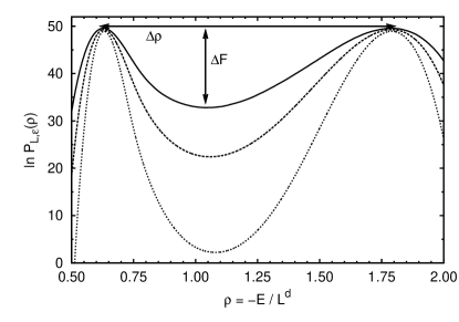
Figure 1: Logarithm of $P_{L,\epsilon}(E)$ using $p=10$ in Eq.(1) for system sizes $L=10,12,15$ (from top to bottom), cubic lattices, and three-dimensional spins. In each of the distributions $\epsilon$ was tuned so the peaks are of equal height. The barrier $\Delta F$, here marked for the $L=10$ system, is defined as the height of the peaks measured with respect to the minimum in between. The peak-to-peak distance $\Delta\rho$ corresponds to the latent heat density. Note that we have plotted the distributions as a function of the negative energy density: the left peak thus corresponds to the isotropic phase and the right peak to the nematic phase.

Figure 2: Variation of $\Delta F$ versus $L^{d-1}$ for $d=3$ dimensional lattices, three-dimensional spins, and the various values of $p$ as indicated.

Figure 3: Similar to Fig. 2 but for two-dimensional lattices and three-dimensional spins.

Figure 4: Similar to Fig. 2 but for two-dimensional lattices and two-dimensional spins.

In order to verify the presence of a first-order transition we use the scaling method of Lee and Kosterlitz physrevlett.65.137 ; citeulike:3908342 . Recall that the order parameter distribution becomes bimodal in the vicinity of the IN transition; see Fig. 1 for an example. The idea of Lee and Kosterlitz is to monitor the peak heights $\Delta F$ of the logarithm of the order parameter distribution, measured with respect to the minimum “in-between” the peaks. At a first-order transition $\Delta F$ corresponds to the formation of interfaces between coexisting isotropic and nematic domains binder:1982 . In $d$ spatial dimensions it is therefore expected that $\Delta F\propto L^{d-1}$, providing a straightforward recipe to identify the transition type: a linear increase of $\Delta F$ versus $L^{d-1}$ indicates that a first-order transition is taking place, with the slope yielding the interfacial tension binder:1982 , whereas for a continuous transition $\Delta F$ becomes independent of $L$, or vanishes altogether if no transition takes place at all in the thermodynamic limit. In Fig. 2 $\Delta F$ is plotted for the purely three-dimensional case; the linear increase is clearly visible, confirming the presence of a first-order transition. For two-dimensional lattices the results have been collected in Fig. 3 and Fig. 4. Once again the presence of a first-order transition is confirmed. Note that on two-dimensional lattices the slopes of the lines correspond to line tensions.

III.2 Extrapolation of $\epsilon_{L,CV}$

Figure 5: Estimation of $\epsilon_{\infty}$ via extrapolation of $\epsilon_{L,CV}$ using Eq.(2). Shown is $\epsilon_{L,CV}$ versus $1/L^{d}$ using (a) $p=10$, cubic lattices and three-dimensional spins, (b) $p=20$, square lattices and three-dimensional spins and (c) $p=150$, square lattices and two-dimensional spins. The open symbols are simulation data and the lines are fits to Eq.(2).

Table 1: Properties of the IN transition of Eq.(1) for three-dimensional lattices and three-dimensional spins versus $p$. Listed are the fit parameters $\epsilon_{\infty,CV}$ and $\alpha$ of Eq.(2), the best estimate $\epsilon_{\infty,k}$ obtained from the convergence of $\epsilon_{L,k}$ along $k_{\rm opt}$, the logarithm of $k_{\rm opt}$ with uncertainty $\Delta k$, the latent heat density ${\cal L}_{\infty}$ and the ratio $\ln k_{\rm opt}/{\cal L}_{\infty}$.

$p$	$\epsilon_{\infty,CV}$	$\alpha$	$\epsilon_{\infty,k}$	$\ln k_{\rm opt}\pm\Delta k$	$\cal L_{\infty}$	$\ln k_{\rm opt}/{\cal L}_{\infty}$
5	1.3969	6.62	$1.3970\pm 0.001$	$2.7\pm 0.6$	$0.358\pm 0.010$	$5.9-9.2$
8	1.5207	5.28	$1.5207\pm 0.001$	$5.0\pm 0.2$	$0.908\pm 0.005$	$5.3-5.7$
10	1.5862	4.28	$1.5864\pm 0.001$	$5.3\pm 0.5$	$1.156\pm 0.005$	$4.2-5.0$
15	1.7126	3.94	$1.7126\pm 0.001$	$6.0\pm 0.2$	$1.523\pm 0.002$	$3.8-4.1$
20	1.8063	3.76	$1.8063\pm 0.001$	$6.4\pm 0.3$	$1.727\pm 0.002$	$3.5-3.9$
45	2.0838	3.55	$2.0838\pm 0.001$	$8.1\pm 1.0$	$2.120\pm 0.001$	$3.3-4.3$

Table 2: Similar to Table 1 but for two-dimensional lattices and three-dimensional spins.

$p$	$\epsilon_{\infty,CV}$	$\alpha$	$\epsilon_{\infty,k}$	$\ln k_{\rm opt}\pm\Delta k$	$\cal L_{\infty}$	$\ln k_{\rm opt}/{\cal L}_{\infty}$
20	2.7695	5.18	$2.7698\pm 0.001$	$4.1\pm 0.4$	$0.7145\pm 0.001$	$5.2-6.3$
25	2.8678	4.84	$2.8679\pm 0.001$	$4.5\pm 0.2$	$0.8900\pm 0.001$	$4.8-5.3$
30	2.9517	4.69	$2.9517\pm 0.001$	$4.8\pm 0.2$	$1.0023\pm 0.001$	$4.6-5.0$
35	3.0240	4.58	$3.0241\pm 0.001$	$5.2\pm 0.6$	$1.0832\pm 0.001$	$4.2-5.4$
40	3.0882	4.52	$3.0882\pm 0.001$	$5.2\pm 0.2$	$1.1432\pm 0.001$	$4.4-4.7$
45	3.1456	4.47	$3.1455\pm 0.001$	$5.2\pm 0.5$	$1.1936\pm 0.001$	$3.9-4.8$
50	3.1976	4.50	$3.1976\pm 0.001$	$5.6\pm 0.5$	$1.2320\pm 0.001$	$4.1-5.0$

Table 3: Similar to Table 1 but for two-dimensional lattices and two-dimensional spins.

$p$	$\epsilon_{\infty,CV}$	$\alpha$	$\epsilon_{\infty,k}$	$\ln k_{\rm opt}\pm\Delta k$	$\cal L_{\infty}$	$\ln k_{\rm opt}/{\cal L}_{\infty}$
150	2.063	3.67	$2.0628\pm 0.0005$	$1.9\pm 0.8$	$0.648\pm 0.005$	$1.7-4.2$
1000	2.486	3.31	$2.4865\pm 0.0006$	$4.8\pm 1.3$	$1.270+0.005$	$2.8-4.8$

Next, we measure the thermodynamic limit inverse temperature $\epsilon_{\infty}$ by means of extrapolating $\epsilon_{L,CV}$ via Eq.(2). Recall that $\epsilon_{L,CV}$ is the finite-size inverse temperature where the specific heat

$$C_{L}=\frac{{\langle E^{2}\rangle}-{\langle E\rangle}^{2}}{L^{d}}$$ (7)

attains its maximum. Shown in Fig. 5(a) is $\epsilon_{L,CV}$ versus $1/L^{d}$ for the purely three-dimensional case using $p=10$ - results for different $p$ are qualitatively similar and therefore not explicitly shown. In agreement with earlier simulations of the “original” LL model physrevlett.69.2803 ; citeulike:3740162 , the data are well described by Eq.(2) and from the fit $\epsilon_{\infty}$ can be meaningfully obtained. The resulting fit parameters are collected in Table 1. Repeating the same analysis for two-dimensional lattices yields similar results; some typical plots are shown in Fig. 5(b) and (c) with the resulting fit parameters collected in Tables II and III.

III.3 Extrapolation of $\epsilon_{L,k}$

We now arrive at the main result of this paper, namely the estimation of $\epsilon_{\infty}$ by monitoring $\epsilon_{L,k}$. Recall that $\epsilon_{L,k}$ is defined as the finite-size inverse temperature where the equality

$$W_{N}/W_{I}=k$$ (8)

is obeyed, with $W_{N}$ and $W_{I}$ the areas under the nematic and isotropic peaks of the order parameter distribution respectively. No matter what value of $k$ is used, provided it is positive and finite, we expect that $\lim_{L\to\infty}\epsilon_{L,k}=\epsilon_{\infty}$. The reason is that in the thermodynamic limit a bimodal order parameter distribution survives only at $\epsilon_{\infty}$ and not anywhere else citeulike:3908342 . Hence, keeping the area ratio fixed at some value of $k$ whilst increasing $L$, $\epsilon_{L,k}$ will definitely approach $\epsilon_{\infty}$. The rate of the convergence, however, does depend on $k$. Assuming that the prediction of Borgs and Kotecky for the Potts model also holds at first-order IN transitions, it should be possible to locate an optimal value $k_{\rm opt}$ at which the convergence to $\epsilon_{\infty}$ is fastest and hopefully faster than $1/L^{d}$. Therefore, we propose to manually inspect the convergence of $\epsilon_{L,k}$ using several values of $k$.

A prerequisite for numerically solving Eq.(8) is that the transition must be sufficiently first-order in order for bimodal distributions $P_{L,\epsilon}(E)$ with well-separated peaks to appear. By this we mean that the barrier $\Delta F$, defined in Fig. 1, is large enough. The areas of the nematic and isotropic peaks may then be calculated using

$$W_{N}=\int_{-\infty}^{E_{c}}P_{L,\epsilon}(E)\,dE,\hskip 5.69054ptW_{I}=\int_{E_{c}}^{0}P_{L,\epsilon}(E)\,dE,$$ (9)

where we remind the reader that the energy in our model is negative. The details of defining the “cut-off” energy $E_{c}$ are somewhat arbitrary, but as states around $E_{c}$ contribute exponentially little to the peak areas, the precise form does not matter citeulike:3596258 . In this work $E_{c}$ is taken to be the average $E_{c}=\int EP_{L,\epsilon}(E)\,dE$, with $P_{L,\epsilon}(E)$ obtained at equal-height, i.e. as in Fig. 1. Once $E_{c}$ has been set its value is kept fixed whilst solving Eq.(8).

Figure 6: Variation of $\epsilon_{L,k}$ versus $L$, for three-dimensional lattices and three-dimensional spins, using different exponents $p$ as indicated. The symbols are simulation data, the lines serve to guide the eye. The central curves in each plot show $\epsilon_{L,k}$ using $k=k_{\rm opt}$ along which finite-size effects are minimal; also shown is $\epsilon_{L,k}$ using $k=k_{\rm opt}-5\Delta k$ (lower curves), and $k=k_{\rm opt}+5\Delta k$ (upper curves). The methods for locating $k_{\rm opt}$ and $\Delta k$ are explained in the text and the resulting values, as well as the estimates of $\epsilon_{\infty}$, are listed in Table 1.

Figure 7: Similar to Fig. 6 but for two-dimensional lattices and three-dimensional spins. Numerical estimates are given in Table 2.

Figure 8: Similar to Fig. 6, but for two-dimensional lattices and two-dimensional spins. Numerical estimates are given in Table 3.

For the purely three-dimensional case, the behaviour of $\epsilon_{L,k}$ is shown in Fig. 6. Using a number of exponents $p$ in Eq.(1), we have plotted $\epsilon_{L,k}$ versus $L$ for several values of $k$. The data are consistent with the expectation that, regardless of $k$, $\epsilon_{L,k}$ converges to a common value, corresponding to $\epsilon_{\infty}$. Note also that $\epsilon_{\infty}$ is approached from above for large $k$, and from below for low $k$. Hence, we can indeed identify an optimal value $k_{\rm opt}$ along which finite-size effects are minimal. The optimum can be estimated by locating, for a pair of system sizes $L_{i}$ and $L_{j}$, the inverse temperature $\epsilon_{ij}$ where for both system sizes the same ratio $k_{ij}$ of the peak areas is observed. By considering all available pairs of system sizes, the average and root-mean-square fluctuation in $\epsilon_{ij}$ and $k_{ij}$ can be calculated, which then yield $\epsilon_{\infty}$ and $k_{\rm opt}$ with uncertainties, shown in Table 1. Although $k_{\rm opt}$ itself is not known very precisely, since $\Delta k$ is quite large, very accurate estimates of $\epsilon_{\infty}$ can still be obtained as this quantity is rather insensitive to the precise value of $k_{\rm opt}$ being used. This means that the series $\epsilon_{L,k}$ also provides a valid method for locating IN transitions. The corresponding estimates of $\epsilon_{\infty}$ are in good agreement with those obtained via extrapolation of $\epsilon_{L,CV}$, as inspection of the various tables indicates. The practical advantage of using $\epsilon_{L,k}$ with $k=k_{\rm opt}$ is that the $L$-dependence is very weak, so much so that $\epsilon_{\infty}$ is captured already in small systems. Similar findings were obtained using two-dimensional lattices, of which some typical plots are provided in Fig. 7 and Fig. 8 with the corresponding numerical estimates collected in Tables II and III.

Figure 9: Plot of $\ln W_{N}/W_{I}$ versus $\epsilon$ for several system sizes $L$. This plot was generated using $p=10$ in Eq.(1), three-dimensional lattices and three-dimensional spins.

For non-optimal values $k\neq k_{\rm opt}$, we observe that the shift $\epsilon_{\infty}-\epsilon_{L,k}\propto 1/L^{d}$, i.e. the shift vanishes as a power law in the inverse volume, similar to $\epsilon_{L,CV}$. At the optimal value $k=k_{\rm opt}$, finite-size effects in $\epsilon_{L,k}$ are typically too small in order for a meaningful fit to be carried out. Hence, our data confirm Borgs and Kotecky in the sense that optimal estimators can be defined which converge onto $\epsilon_{\infty}$ faster than $1/L^{d}$; whether the optimal convergence is indeed exponential requires more accurate data, which is currently beyond our reach note3 .

An alternative, but completely equivalent, method to investigate the convergence of $\epsilon_{L,k}$ is presented in citeulike:3596176 ; citeulike:3596258 ; citeulike:3608409 ; citeulike:3610966 , albeit for the Potts model. The idea is to plot the area ratio $W_{N}/W_{I}$ versus $\epsilon$ for several system sizes. The resulting curves are expected to reveal an intersection point at the transition inverse temperature; the value of the area ratio at the intersection then yields $k_{\rm opt}$. For completeness we have prepared one such plot, see Fig. 9. The curves indeed intersect and give estimates of $\epsilon_{\infty}$ and $k_{\rm opt}$ that are fully consistent with those reported in Table I.

III.4 Latent heat density

It appears that scaling relations derived for the Potts model also work remarkably well at IN transitions. In agreement with earlier simulations of the LL model physrevlett.69.2803 ; citeulike:3740162 , the validity of Eq.(2) is confirmed additionally by us. Furthermore, our data suggest that an analogue of the Borgs and Kotecky prediction, namely that finite-size effects vanish faster than $1/L^{d}$ at appropriate points, can be defined. In this case, it is needed to measure $\epsilon_{L,k}$ using the optimal value $k=k_{\rm opt}$. In the Potts model it holds that $k_{\rm opt}=q$, where $q$ is the number of Potts states. In other words, finite-size effects in the Potts model are minimized when the ratio of the peak areas in the order parameter distribution is held fixed at $q$. Based on our results, it seems reasonable to assume that scaling relations for the Potts model also hold at IN transitions, but with $q$ replaced by $k_{\rm opt}$.

Figure 10: Finite-size variation of the latent heat density estimators $\Delta\rho_{L,1}$ and $\Delta\rho_{L,2}$. Results are shown for Eq.(1) using (a) $p=10$, three-dimensional lattices and three-dimensional spins, (b) $p=20$, two-dimensional lattices and three-dimensional spins and (c) $p=150$, two-dimensional lattices and two-dimensional spins.

To test this assumption we consider the proportionality constant $\alpha$ from Eq.(2), which is given by Eq.(3) for the Potts model. If $q$ can be replaced by $k_{\rm opt}$, $\alpha$ should correspond to $\ln k_{\rm opt}/{\cal L}_{\infty}$, where ${\cal L}_{\infty}$ is the latent heat density. The latter can be obtained independently from $C_{L,\rm max}={\cal L}_{\infty}^{2}L^{d}/4$, where $C_{L,\rm max}$ is the maximum value of the specific heat in a finite system of size $L$ citeulike:3720308 . Hence, we introduce the latent heat estimator

$$\Delta\rho_{L,1}=\sqrt{4C_{L,\rm max}/L^{d}},$$ (10)

which should approach ${\cal L}_{\infty}$ as $L\to\infty$. Additionally, the latent heat density can be read-off directly, as the peak-to-peak distance in the energy distribution, marked $\Delta\rho$ in Fig. 1. Numerically this is expressed by ${\cal M}_{L}=2{\langle|E-{\langle E\rangle}|\rangle}/L^{d}$; plotting ${\cal M}_{L}$ versus $\epsilon$ gives a maximum $\Delta\rho_{L,2}$, which in the limit $L\to\infty$ also approaches ${\cal L}_{\infty}$. Typical behaviour of $\Delta\rho_{L,i}$ is shown in Fig. 10. As expected, both latent heat estimators converge to a common value, which can be read-off reasonably accurately; the resulting estimates of ${\cal L}_{\infty}$ are given in the various tables. Note also that ${\cal L}_{\infty}$ is approached from below in three dimensions, whereas in two dimensions, it is approached from above. If an appropriate number of two-dimensional lattice layers stacked on top of each other were simulated, it is likely that a cross-over regime could be found where $\Delta\rho_{L,i}$ depends only weakly on $L$, as these systems are effectively in-between two and three dimensions.

Having measured ${\cal L}_{\infty}$, the ratio $\ln k_{\rm opt}/{\cal L}_{\infty}$ is easily obtained, which may then be compared to $\alpha$, see Tables I-III. The uncertainty is admittedly rather large, but within numerical precision, and the relation $\ln k_{\rm opt}/{\cal L}_{\infty}\sim\alpha$ appears to hold.

IV Summary

In this paper we have presented simulation data of first-order isotropic-to-nematic transitions in lattice liquid crystals with continuous orientational degrees of freedom for various space and spin dimensions. As with earlier simulations of this type physrevlett.69.2803 ; citeulike:3740162 , we find that the extrapolation of the finite-size inverse temperature of the specific heat maximum $\epsilon_{L,CV}$ can be consistently performed assuming a leading $\alpha/L^{d}$ dependence, exactly as in the Potts model. Inspired by this result, we have investigated an alternative approach to locate the transition inverse temperature using estimators $\epsilon_{L,k}$, defined as the finite-size inverse temperature where the ratio of peak areas in the energy distribution is equal to $k$. In agreement with the Potts model, $\epsilon_{L,k}$ converges to $\epsilon_{\infty}$ much faster than $1/L^{d}$, provided an optimal value $k=k_{\rm opt}$ is used. Moreover, the ratio $k_{\rm opt}/{\cal L}_{\infty}$, with ${\cal L}_{\infty}$ the latent heat density, is remarkably consistent with the proportionality constant $\alpha$ from the scaling of $\epsilon_{L,CV}$. This leads us to conclude that finite-size scaling predictions originally proposed for first-order transitions in the Potts model remain valid at first-order IN transitions too, but with the number of Potts states $q$ replaced by $k_{\rm opt}$.

It is perhaps somewhat surprising that a continuous spin model at a first-order transition, such as the LL model, scales in the same way as the Potts model, which is, after all, a discrete spin model. In fact, Borgs and Kotecky have remarked that the derivation of their scaling results cannot be easily extended to continuous spin models borgs.kotecky:1992 . Nevertheless, the LL model and its variants may be more closely connected to the Potts model than one may initially think. Note that for large $p$ the Hamiltonian of Eq.(1) becomes increasingly Potts-like, in the sense that the pair interaction approaches a $\delta$-function: $\lim_{p\to\infty}|\vec{d}_{i}\cdot\vec{d}_{j}|^{p}=\delta(\vec{d}_{i},\vec{d}_{j})$. This implies that neighbouring spins only interact when they are closely aligned and are otherwise indifferent to each other, just as in the Potts model. It has indeed been suggested that such models approximately resemble $q$-state Potts models, with $q\sim\sqrt{p}$ physrevlett.52.1535 . The observed trends in this work are certainly consistent with this interpretation. For all cases considered the strength of the transition increases with $p$, as manifested by the growing latent heats and interfacial tensions, exactly as in the Potts model with increasing $q$. Also the upward shift of $\epsilon_{\infty}$ with $p$ is consistent with the Potts model. However, it is clear that new theoretical approaches are needed to fully understand finite-size effects at first-order transitions in the models studied here. We hope that the present simulation results may inspire such efforts.

- (1) P. A. Lebwohl and G. Lasher, Physical Review A 6, 426+ (1972).
- (2) U. Fabbri and C. Zannoni, Molecular Physics 58, 763 (1986).
- (3) C. M. Care and D. J. Cleaver, Reports on Progress in Physics 68, 2665 (2005).
- (4) M. A. Bates and D. Frenkel, The Journal of Chemical Physics 112, 10034 (2000).
- (5) D. Frenkel and R. Eppenga, Phys. Rev. A 31, 1776 (1985).
- (6) H. Kunz and G. Zumbach, Physical Review B 46, 662+ (1992).
- (7) R. L. C. Vink, Physical Review Letters 98, 217801+ (2007).
- (8) H. H. Wensink and R. L. C. Vink, Journal of Physics: Condensed Matter 19, 466109+ (2007).
- (9) E. Domany, M. Schick, and R. H. Swendsen, Phys. Rev. Lett. 52, 1535 (1984).
- (10) A. C. D. van Enter and S. B. Shlosman, Phys. Rev. Lett. 89, 285702 (2002).
- (11) A. C. D. van Enter, S. Romano, and V. A. Zagrebnov, J. Phys. A 39 (2006).
- (12) K. Binder, Reports on Progress in Physics 60, 487 (1997).
- (13) The exceptions appear to be: M. Fisher and V. Privman, J. Appl. Phys. 57, 3327 (1985); Phys. Rev. B 32, 447 (1985); Commun. Math. Phys. 103, 527 (1986).
- (14) M. S. Challa, D. P. Landau, and K. Binder, Physical Review B 34, 1841+ (1986).
- (15) C. Borgs, R. Kotecký, and S. Miracle-Solé, Journal of Statistical Physics 62, 529 (1991).
- (16) Z. Zhang, O. G. Mouritsen, and M. J. Zuckermann, Phys. Rev. Lett. 69, 2803 (1992).
- (17) N. V. Priezjev and R. A. Pelcovits, Physical Review E 63, 062702+ (2001).
- (18) F. Y. Wu, Rev. Mod. Phys. 54, 235 (1982).
- (19) C. Borgs and R. Kotecký, Journal of Statistical Physics 61, 79 (1990).
- (20) C. Borgs and R. Kotecky, Phys. Rev. Lett. 68, 1734 (1992).
- (21) Strictly speaking, Eq.(2) also requires a strong enough first-order transition. For example, in the derivation of Ref. citeulike:3716330, , it is assumed that the order parameter distribution consists of two non-overlapping Gaussians.
- (22) K. Vollmayr, J. D. Reger, M. Scheucher, and K. Binder, Zeitschrift für Physik B Condensed Matter 91, 113 (1993).
- (23) C. Chiccoli, P. Pasini, and C. Zannoni, Physica A: Statistical and Theoretical Physics 148, 298 (1988).
- (24) R. Garcia, E. Subashi, and M. Fukuto, Physical Review Letters 100, 197801+ (2008).
- (25) F. Wang and D. P. Landau, Physical Review Letters 86, 2050+ (2001).
- (26) F. Wang and D. P. Landau, Physical Review E (Statistical, Nonlinear, and Soft Matter Physics) 64 (2001).
- (27) J.-S. Wang and R. H. Swendsen, Journal of Statistical Physics 106, 245 (2002).
- (28) S. M. Shell, P. G. Debenedetti, and A. Z. Panagiotopoulos, The Journal of Chemical Physics 119, 9406 (2003).
- (29) Q. Yan and J. J. de Pablo, Physical Review Letters 90, 035701+ (2003).
- (30) B. J. Schulz, K. Binder, M. Müller, and D. P. Landau, Physical Review E 67, 067102+ (2003).
- (31) J. Lee and J. M. Kosterlitz, Phys. Rev. Lett. 65, 137 (1990).
- (32) J. Lee and J. M. Kosterlitz, Physical Review B 43, 3265+ (1991).
- (33) K. Binder, Phys. Rev. A 25, 1699 (1982).
- (34) W. Janke, Physical Review B 47, 14757+ (1993).
- (35) For the Potts model, the exponential size dependence has been accurately resolved citeulike:3610966 .
- (36) C. Borgs and W. Janke, Physical Review Letters 68, 1738+ (1992).
- (37) W. Janke, in Computer Simulations in Condensed Matter Physics VII, edited by D. P. Landau, K. K. Mon, and H. B. Schuettler, pages 29+ (Springer-Verlag, Berlin, Heidelberg, 1994).
- (38) A. Billoire, R. Lacaze, and A. Morel, Nuclear Physics B 370, 773 (1992).