Transit mapping of a starspot on CoRoT-2

We analyze variations in the transit lightcurves of CoRoT-2b, a massive hot Jupiter orbiting a highly active G star. We use one transit lightcurve to eclipse-map a photospheric spot occulted by the planet. In this case study we determine the size and longitude of the eclipsed portion of the starspot and systematically study the corresponding uncertainties. We determine a spot radius between $4.5\degr$ and $10.5\degr$ on the stellar surface and the spot longitude with a precision of about $\pm 1$ degree. Given the well-known transit geometry of the CoRoT-2 system, this implies a reliable detection of spots on latitudes typically covered by sunspots; also regarding its size the modelled spot is comparable to large spot groups on the Sun. We discuss the future potential of eclipse mapping by planetary transits for the high-resolution analysis of stellar surface features.

1 Introduction

The atmosphere of the Sun shows inhomogeneities down to the smallest scales currently accessible to solar observations which are of the order of 50 km (e.g. Scharmer et al., 2002). Such intricate fine structure can also be expected in the atmospheres of other active stars. However, the best currently available stellar observations only resolve surface features down to the size of a few degrees on the surface, corresponding to several 10000 km on a main sequence star.

The increasing number of known transiting extrasolar planets offers an outstanding opportunity to study surface inhomogeneities of their host stars with an unprecedented surface resolution. As an example of this new technique, we present the analysis of one transit lightcurve of the planetary system CoRoT-2, recently detected by the CoRoT satellite (Rouan et al.,, 1998). Our study indicates that under favourable conditions the CoRoT lightcurves allow the study of e.g. starspots and/or faculae down to a sub-degree scale on the stellar surface.

Deformations of planetary transit lightcurves, attributable to dark spots, have been observed for several systems: HD 189733, Pont et al., 2007; HD 209458, Silva-Valio, 2008; Tres-1, Rabus et al., 2009 and CoRoT-2, Lanza et al., 2009. Especially, Pont et al.,’s study, based on HST data, for the first time showed that low-noise transit photometry of exoplanets can yield detailed information about surface features of their host star. We present a systematic analysis of the spot locations and extensions, including their uncertainties, that can be deduced from transit lightcurves.

CoRoT-2a (GSC 00465-01282) is an apparently young late G-dwarf star (Alonso et al., 2008, AL08 in the following); it is unsually active and intrinsically variable among the presently known planetary host stars. Its rotation period of $P_{\ast}=4.52\pm 0.14\leavevmode\nobreak\ d$ (Lanza et al., 2009) amounts to less than three times the planetary orbit period $P_{orb}$: $13\cdot P_{orb}=5.004\cdot P_{\ast}$. Densely sampled high-precision photometry in combination with spectroscopic measurements make the transit geometry of CoRoT-2b exceptionally well known (AL08, Bouchy et al., 2008): The planet is on a nearly circular orbit ($e=0.003\pm 0.003$) which is seen close to edge-on ($i=87.84\pm 0.10\degr$) and approximately oriented perpendicular to the stellar rotation axis (deviating by $\lambda=7.2\pm 4.5\degr$).

These attributes turn the planetary disk into an extremely well-defined probe which periodically scans a band on the stellar surface covering $20\degr$ in latitude. The orbital period of CoRoT-2b translates into an orbital angular velocity of 0.002 deg/s. As a result, close to the center of the stellar disk, the planet moves $\approx 0.1$ deg in longitude during a 32 s time bin of the CoRoT data. By order of magnitude, this value then determines the attainable surface resolution of the CoRoT observations of CoRoT-2.

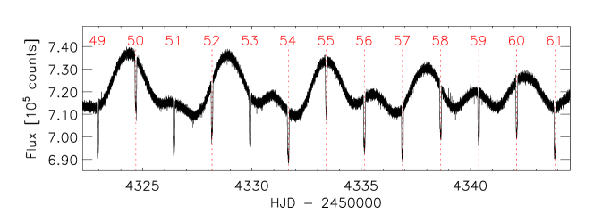
Figure 1: Section of the CoRoT lightcurve of CoRoT-2, purged of outlying values (see Sect. 2). The transits appear as recurrent dips overlying the modulation by the stellar rotation. Transits are numbered from the beginning of the CoRoT observations, our analysis focusses on transit no. 56.

2 Observations and data analysis

The CoRoT (Auvergne et al.,, 2009) lightcurve of CoRoT-2 observed from 2007 May 16 to 2007 October 15 continuously samples 31 stellar rotations. After five days of observations the satellite’s sampling cadence of CoRoT-2 was switched from 512 s to 32 s, resulting in a lightcurve that covers 79 planetary transits at this high time resolution.

Our analysis started out from the lightcurve data as delivered by the CoRoT pipeline. The pipeline sorts out defective data (e.g. due to crossings of the South Atlantic Anomaly, SAA) and performs a background subtraction. As a first step we added up all three CoRoT photometry channels (red-green-blue) into a single lightcurve, because the individual channels are more affected by instrumental instabilities than their summed-up signal.

Similar to AL08, we then removed outlier points which show a pronounced non-normal distribution. To this end we computed the standard deviation $\sigma$ in several narrow intervals, yielding $\sigma\approx 950$. We discarded all points deviating more than $3\sigma$ from a boxcar-smoothed copy of the lightcurve, thus rejecting nearly 2% of all points. Finally, also following AL08, we corrected for the $5.6\%$ contamination by a neighbouring object; a subinterval of the resulting lightcurve is shown in Fig. 1.

The transits occur during different stellar rotation phases, i.e. at different levels and slopes of the lightcurve. In order to compare the transit lightcurves, it is convenient to normalize them to a common level. To this end, we carried out a linear interpolation of points adjacent to each transit and divided all transit lightcurves by their interpolating function. One lightcurve normalized in this way is shown in Fig. 2.

We note that this procedure introduces a systematic error that depends on the spot coverage of the stellar disk visible during the transit. If, e.g., the disk is covered by dark spots not occulted by the planet, the transit depth will not yield the true ratio of radii $R_{planet}/R_{\ast}$. Instead, the stellar radius $R_{\ast}$ will be underestimated relative to the planet, because part of the stellar disk is dark and essentially invisible. Given the typical amplitude of CoRoT-2’s lightcurve of about 4% peak-to-peak, this introduces a comparable uncertainty for the planetary radius deduced from a single transit. Consequently, this uncertainty also affects our spot size estimate of the next section. We will discuss the influence of activity-induced lightcurve variations on the determination of planetary parameters in a forthcoming paper.

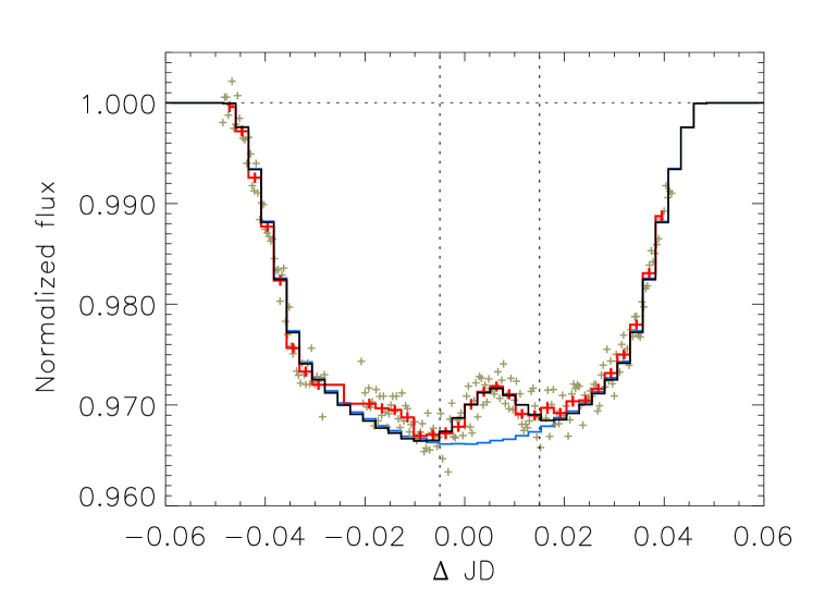
Figure 2: Normalized lightcurve during “transit 56”, as a function of time from the transit center. Gray symbols indicate the unbinned measurements, the red line shows them averaged in 224 sec time bins with 1$\sigma$-errors indicated. The vertical lines delimit the time interval used for our spot model; the lightcurve fit resulting from our model is drawn black (model “BN” in Table 1). The blue line shows the transit model for an unspotted star for comparison. The shallow deformation left of the transit center is caused by another spot not included in our model.

3 Transit lightcurve modelling

To determine a spot configuration compatible with the deformations of a transit lightcurve, we selected one particular transit occuring close to JD 2454335.0 and referred to as “transit 56”. Rendered in Fig. 2, it shows the most pronounced and isolated “bump” of the whole time series of CoRoT-2, suggesting a relatively narrow spot occulted close to the disk center. Additionally, the symmetry of the bump indicates a spot geometry that is largely symmetric in longitude.

3.1 The model

To model a transit lightcurve we decompose the stellar surface into roughly square elements. The integrated stellar flux is computed by summing up the fluxes of all visible elements, respecting their projected area and the limb darkening (e.g. Wolter et al., 2005). To model the planetary transit, all surface elements occulted by the planetary disk at a given phase are removed from the sum, thus treating the planet as a circular disk without any intrinsic emission. The surface resolution needs to be sufficient to analyze the densely sampled movement of the planetary disk over the stellar surface. We choose a surface grid with 750 elements at the equator, yielding 178 868 elements in total and a surface resolution of roughly $0.5\degr$ near the equator. Also, this high resolution is required to compute lightcurve models sufficiently free of jitter, not exceeding a few $10^{-4}$ in our models.

Next, we adjusted the limb darkening to optimize the fit to the transit ingress and egress as well as to a tentative lower envelope of transit 56 and the surrounding transits. We adopt a linear limb-darkening law with $\epsilon=0.6$; we note, however, that this has little influence on our determined spot parameters since the spot occultation in transit 56 occurs close to the disk center.

We compute the position of the planetary disk on the stellar disk and the corresponding stellar rotation phase using the orbital parameters and planetary size given by AL08, as well as a stellar rotation period of $P_{\ast}=4.5284$ d, determined by a periodogram analysis and compatible with the value of Lanza et al., (2009), adopting the lightcurve maximum at JD 2454242.67 as phase zero point. To this end, we introduce Cartesian coordinates in units of the stellar radius $R_{\ast}$ with their origin at the center of the star and the observer located on the $x$-axis. The stellar rotation axis is assumed to coincide with the $z$-axis, while the axis of the planetary orbit is tilted by $90\degr-i=2.2\degr$ in the $xz$-plane. Both, the stellar rotation and the planetary orbit are adopted as right-handed around the $z$-axis.

Using these coordinates, $z_{pl}$ and $y_{pl}$ describe the position of the center of the planetary disk projected onto the stellar disk visible at the stellar rotation phase $\phi$. The following relations apply:

$$\hskip 21.52771ptz_{pl}=\cos{i\cdot a/R_{\ast}}\\$$ (1)

where $i$ and $a$ describe the inclination and the semimajor axis of the planetary orbit, respectively.

$$\hskip 21.52771pt\phi-\phi_{cen}=\frac{y_{pl}}{y_{IV}}\cdot\frac{\tau_{trans}}{P_{\ast}}$$ (2)

where $\phi_{cen}$ is the stellar rotation phase at transit center, while $\tau_{trans}$ and $P_{\ast}$ give the transit duration (first to last contact) and the stellar rotation period, respectively. $\tau_{trans}=8200$ s can be computed using Eq. (4) of Charbonneau et al., (2006). $y_{IV}$ describes the lateral planet position at last contact

$$\hskip 21.52771pty_{IV}=\sqrt{\left(1+R_{pl}/R_{\ast}\right)^{2}-z_{pl}^{2}}$$ (3)

with $R_{pl}$ giving the planetary radius. Note that Eq. 2 is only strictly valid for $R_{\ast}\ll a$; however, the error is of the order of $(R_{\ast}/a)^{2}$ and can be neglected for our analysis. In addition, Eq. 1 does not include the projected angle between the stellar rotation axis and the planetary orbital axis $\lambda$. However, given Bouchy et al., (2008)’s value of $\lambda\approx 7\degr$ and the proximity of the modelled spot to the disk center, this introduces an uncertainty of less than $2\degr$ for the spot latitude.

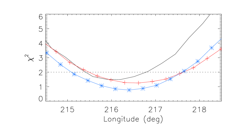
Figure 3: Fit quality of our transit lightcurve models as a function of spot longitude, shown for the models BC (blue stars), BN (red plus symbols) and DS (black curve), of Table 1. Our adopted limiting value of $\chi^{2}=2.0$ is marked by the dotted line.

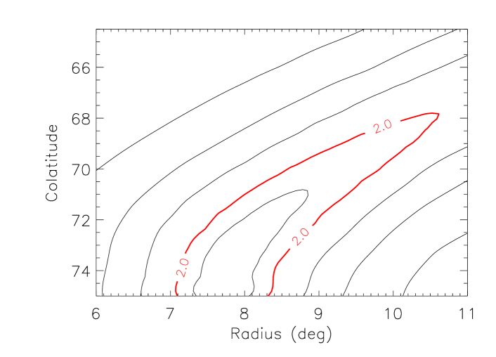
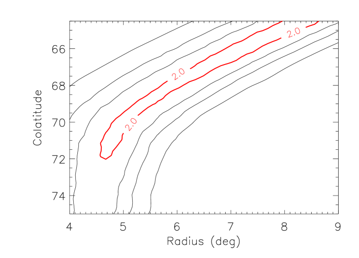
Figure 4: Fit quality $\chi^{2}$ of our transit lightcurve models as a function of the spot radius and its center colatitude. The upper panel describes the “bright spot” scenario (models BC, BN and BS of Table 1), while the lower panel applies to the “dark spot” solutions (models DN and DS). Subsequent contours mark levels of $\chi^{2}=1,2,5,10$ and $20$; the adopted limiting contour, $\chi^{2}=2$, is drawn bold red. Because of the near symmetry of the $\chi^{2}$-contours, only colatitudes in the upper half of the transit band are shown. See text for discussion.

3.2 Transit mapping of a starspot

Our initial tests showed that the given transit lightcurves do not significantly constrain the spot shape and contrast. Hence we limit our models to circular spots or circle segments. Furthermore, we tentatively adopt two values for the spot-to-photosphere contrast: As a “dark spot” scenario we choose a spot flux of 30% of the photospheric flux. Based on Bouchy et al., (2008)’s effective temperature of CoRoT-2a of $5625$ K and Planck’s law at a wavelength of $6000$ Å, this corresponds to a spot approximately $1200$ K cooler than the photosphere. This is motivated by spot temperatures found for other highly active G and K stars (e.g. Strassmeier & Rice, 1998, O’Neal et al., 2004). As a “bright spot” we adopt a value of 75% of the photospheric flux. This roughly represents the average contrast of large spot groups on the Sun at visible wavelengths (Walton et al., 2003, Albregtsen et al., 1984). Our two spot contrast scenarios are comparable to those adopted for CoRoT-2a by Lanza et al., (2009).

Defining the spot contrast and shape in this way, three free parameters describe a given spot, namely the spot radius $r$ as well as its central longitude $\varphi$ and colatitude $\theta$. However, as illustrated by Fig. 3, the longitude is closely confined by the transit lightcurve, irrespective of the spot contrast and colatitude. This is due to the well defined maximum of the transit bump. Thus only two undetermined parameters remain to optimize the fit of transit 56’s lightcurve: $r$ and $\theta$. We calculated model lightcurves for grids in these two parameters, the resulting goodness-of-fit $\chi^{2}$ is shown in Fig. 4.

To calculate $\chi^{2}$ we rebinned the lightcurve into 224 sec bins, and estimated the resulting errors $\sigma_{j}$ assuming Gaussian error propagation: $\chi^{2}={1}/{(N-M)}\cdot{\sum_{j=1}^{N}\left(F_{obs,j}-F_{model,j}\right)^{2}}/{\sigma_{j}^{2}}$ . Here, $M=3$ is the number of free model parameters, namely the spot longitude, colatitude and radius. $N=8$ gives the number of time bins used to constrain the modelled spot, see the interval limits indicated in Fig. 2.

Reducing $\chi^{2}$ in this way is non-unique because of the significant correlation of the spot radius and colatitude, illustrated by the slanted contours of Fig. 4. Tentatively we choose a limit of $\chi^{2}\leq 2.0$ for models judged as compatible with the observations. As an example, Fig. 2 shows a solution yielding $\chi^{2}=1.4$.

3.3 Results

As the $\chi^{2}$-contours in the upper panel of Fig. 4 show, for the “bright spot” scenario, the central spot colatitude is confined to $\theta=75\pm 6\degr$, i.e. inside the stellar surface belt transited by the planet. The spot radii are slightly smaller than, or comparable to, the size of the planetary disk: $r=7.1\degr\ldots 10.6\degr$. This scenario is illustrated by Fig. 5 and the exemplary solutions BN, BC and BS (“bright north, central and south ”) of Table 1.

For the “dark spot” scenario, on the other hand, only spot centers away from the center of the transit belt yield proper fits to the transit lightcurve: $\theta\leq 72\degr$ and $\theta\geq 78\degr$. This is illustrated by the lower panel of Fig. 4 which also shows that the resulting spot radii are smaller than in the “bright spot” case ($r=4.6\degr\ldots 7.8\degr$).

Also spots with centers outside the transit band yield feasible solutions. An example is illustrated by the red arc in Fig. 5, showing solution DEQ of Table 1. As illustrated by the figure, concerning area and longitude extent they do not differ significantly from solutions with centers inside the band. We do not discuss them further since their radii do not describe the transited extension and area of the spot appropriately.

Table 1: Parameters of characteristic spot solutions discussed in the text, longitudes and colatitudes are given for the spot center.

Model	Long.	Colat.	Radius	Flux	$\chi^{2}$	Area
BC	$216.4\degr$	$75.0\degr$	$7.8\degr$	$0.75$	0.8	0.45%
BN	$216.5\degr$	$70.0\degr$	$9.5\degr$	$0.75$	1.4	0.55%
BS	$216.2\degr$	$80.0\degr$	$8.5\degr$	$0.75$	1.2	0.47%
DN	$216.7\degr$	$71.0\degr$	$4.8\degr$	$0.3$	1.7	0.18%
DS	$216.2\degr$	$81.0\degr$	$4.8\degr$	$0.3$	1.9	0.18%
DEQ	$216.3\degr$	$94.0\degr$	$15.3\degr$	$0.3$	1.6	0.72%

4 Discussion

The shape of the transit lightcurves of CoRoT-2 exhibits highly significant variations between different transits. This indicates a ubiquitous presence of starspots in the surface regions transited by the planet. Furthermore, as illustrated by Fig. 1 and the analysis of Lanza et al., (2009) the overall lightcurve of CoRoT-2 continuously changes in amplitude during the complete CoRoT observations. This shows that the stellar surface of CoRoT-2a persistently evolves on timescales shorter than its rotation period. Such a fast spot evolution is interesting physically and makes CoRoT-2a a favourable case for the study of stellar activity, potentially a landmark system.

We concentrate our analysis on a single planetary transit whose lightcurve shows a pronounced and isolated bump close to the transit center. Assuming this bump is caused by a circular starspot, we determine parameter ranges for this spot which reproduce the observed transit lightcurve.

While, similar to Pont et al.,’s analysis of HD189733, the spot contrast is only weakly constrained, the spot longitude and radius are closely confined by the transit lightcurve. The spot thus reconstructed on CoRoT-2b is comparable in extent with large spot groups on the Sun which cover up to about 1% of the solar surface (Baumann & Solanki,, 2005; Norman,, 2005).

Given the nearly $90\degr$ inclination of CoRoT-2b’s orbit, the transit-covered belt on its surface lies close to the equator. Our analysis proves that CoRoT-2a, like the Sun, exhibits spots in this region. Such well-constrained latitude measurements near the equator are difficult or impossible with other surface reconstruction methods like Doppler imaging. Using long-term transit observations, this may allow to study activity cycles analog to the solar butterfly diagram. Also, concerning possible indications of differential rotation on CoRoT-2a (Lanza et al.,, 2009), the spots in the transit-covered belt could supply additional information.

Solar umbrae have diameters up to about 10 Mm, corresponding to one degree in heliographic coordinates; penumbrae reach approximately twice this size. Our study indicates that a surface resolution of potentially better than one degree can be achieved for host stars of eclipsing planets when applying transit mapping to low-noise and fast-sampled lightcurves. Thus, such observations offer a new opportunity to study “solar-like” surface structures on other stars, they may for example allow to measure the umbra/penumbra contrasts of their spots.

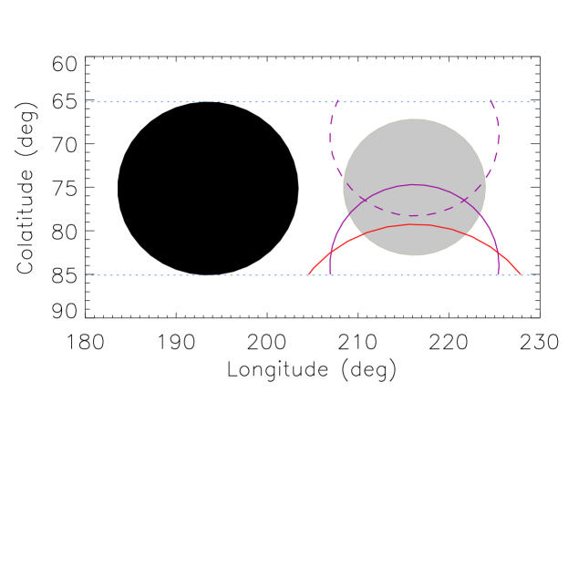
Figure 5: A starspot on CoRoT-2a occulted by the planet during transit 56, as reconstructed by transit mapping. The black and gray circles represent the planetary disk and the spot for our “bright spot” scenario, i.e. adopting a spot flux of 75% relative to the photosphere. The purple arcs illustrate the northern- and southernmost solutions for this spot flux. The red arc illustrates a “dark spot” solution (DEQ in Table 1), see text for discussion.