Optimal waveform estimation for classical and quantum systems via time-symmetric smoothing

Abstract

Classical and quantum theories of time-symmetric smoothing, which can be used to optimally estimate waveforms in classical and quantum systems, are derived using a discrete-time approach, and the similarities between the two theories are emphasized. Application of the quantum theory to homodyne phase-locked loop design for phase estimation with narrowband squeezed optical beams is studied. The relation between the proposed theory and Aharonov et al.’s weak value theory is also explored.

I Introduction

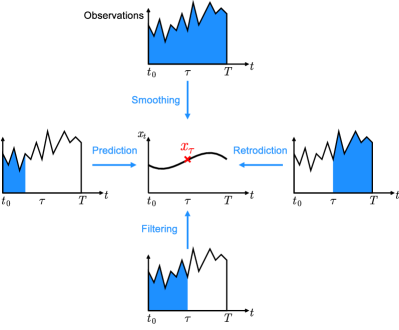
Figure 1: (Color online). Four classes of estimation problems, depending on the observation time interval relative to $\tau$, the time at which the signal is to be estimated.

Estimation theory is the science of determining the state of a system, such as a dice, an aircraft, or the weather in Boston, from noisy observations jazwinski ; vantrees ; crassidis ; simon . As shown in Fig. 1, estimation problems can be classified into four classes, namely, prediction, filtering, retrodiction, and smoothing. For applications that do not require real-time data, such as sensing and communication, smoothing is the most accurate estimation technique.

I have recently proposed a time-symmetric quantum theory of smoothing, which allows one to optimally estimate classical diffusive Markov random processes, such as gravitational waves or magnetic fields, coupled to a quantum system, such as a quantum mechanical oscillator or an atomic spin ensemble, under continuous measurements tsang_smooth . In this paper, I shall demonstrate in more detail the derivation of this theory using a discrete-time approach, and how it closely parallels the classical time-symmetric smoothing theory proposed by Pardoux pardoux . I shall apply the theory to the design of homodyne phase-locked loops (PLL) for narrowband squeezed optical beams, as previously considered by Berry and Wiseman berry . I shall show that their approach can be regarded as a special case of my theory, and discuss how their results can be generalized and improved. I shall also discuss the weak value theory proposed by Aharonov et al. aav in relation with the smoothing theory, and how their theory may be regarded as a smoothing theory for quantum degrees of freedom. In particular, the smoothing quasiprobability distribution proposed in Ref. tsang_smooth is shown to naturally arise from the statistics of weak position and momentum measurements.

This paper is organized as follows: In Sec. II, Pardoux’s classical time-symmetric smoothing theory is derived using a discrete-time approach, which is then generalized to the quantum regime for hybrid classical-quantum smoothing in Sec. III. Application of the hybrid classical-quantum smoothing theory to PLL design is studied in Sec. IV. The relation between the smoothing theory and Aharonov et al.’s weak value theory is then discussed in Sec. V. Sec. VI concludes the paper and points out some possible extensions of the proposed theory.

II Classical smoothing

II.1 Problem statement

Figure 2: (Color online). The classical smoothing problem.

Consider the classical smoothing problem depicted in Fig. 2. Let

$$x_{t} \equiv\left[\begin{array}[]{c}x_{1t}\\ x_{2t}\\ \vdots\\ x_{nt}\end{array}\right]$$ (5)

be a vectoral diffusive Markov random process that satisfies the system Itō differential equation jazwinski

$$dx_{t} =A(x_{t},t)dt+B(x_{t},t)dW_{t},$$ (6)

where $dW_{t}$ is a vectoral Wiener increment with mean and covariance matrix given by

$$\left\langle dW_{t}\right\rangle =0,$$ (7)

$$\left\langle dW_{t}dW_{t}^{T}\right\rangle =Q(t)dt.$$ (8)

The superscript ^T denotes the transpose. The vectoral observation process $dy_{t}$ satisfies the observation Itō equation

$$dy_{t} =C(x_{t},t)dt+dV_{t},$$ (9)

where $dV_{t}$ is another vectoral Wiener increment with mean and covariance matrix given by

$$\left\langle dV_{t}\right\rangle =0,$$ (10)

$$\left\langle dV_{t}dV_{t}^{T}\right\rangle =R(t)dt.$$ (11)

For generality and later purpose, $dW_{t}$ and $dV_{t}$ are assumed to be correlated, with covariance

$$\left\langle dW_{t}dV_{t}^{T}\right\rangle =S(t)dt.$$ (12)

Define the observation record in the time interval $[t_{1},t_{2})$ as

$$dy_{[t_{1},t_{2})} \equiv\left\{dy_{t},t_{1}\leq t<t_{2}\right\}.$$ (13)

The goal of smoothing is to calculate the conditional probability density of $x_{\tau}$, given the observation record $dy_{[t_{0},T)}$ in the time interval $t_{0}\leq\tau\leq T$.

It is more intuitive to consider the problem in discrete time first. The discrete-time system and observation equations (6) and (9) are

$$\delta x_{t} =A(x_{t},t)\delta t+B(x_{t},t)\delta W_{t},$$ (14)

$$\delta y_{t} =C(x_{t},t)\delta t+\delta V_{t}.$$ (15)

The observation record

$$\delta y_{[t_{0},T-\delta t]} \equiv\left\{\delta y_{t_{0}},\delta y_{t_{0}+\delta t},\dots,\delta y_{T-\delta t}\right\}$$ (16)

also becomes discrete. The covariance matrices for the increments are

$$\left\langle\delta W_{t}\delta W_{t}^{T}\right\rangle =Q(t)\delta t,$$ (17)

$$\left\langle\delta V_{t}\delta V_{t}^{T}\right\rangle =R(t)\delta t,$$ (18)

$$\left\langle\delta W_{t}\delta V_{t}^{T}\right\rangle =S(t)\delta t,$$ (19)

and the increments at different times are independent of one another. Because $\delta W_{t}$ and $\delta V_{t}$ are proportional to $\sqrt{\delta t}$, one should keep all linear and quadratic terms of the Wiener increments in an equation according to Itō calculus when taking the continuous time limit.

With correlated $\delta W_{t}$ and $\delta V_{t}$, it is preferable, for technical reasons, to rewrite the system equation (14) as crassidis

$$\delta x_{t} =A(x_{t},t)\delta t+B(x_{t},t)\delta W_{t}$$

$$\quad+D(x_{t},t)\left[\delta y_{t}-C(x_{t},t)\delta t-\delta V_{t}\right],$$ (20)

where $D(x_{t},t)$ can be arbitrarily set because the expression in square brackets is zero. The system equation becomes

$$\delta x_{t} =\left[A(x_{t},t)-D(x_{t},t)C(x_{t},t)\right]\delta t+D(x_{t},t)\delta y_{t}$$

$$\quad+B(x_{t},t)\delta W_{t}-D(x_{t},t)\delta V_{t}.$$ (21)

The new system noise is

$$\delta Z_{t} \equiv B(x_{t},t)\delta W_{t}-D(x_{t},t)\delta V_{t},$$ (22)

$$\left\langle\delta Z_{t}\delta Z_{t}^{T}\right\rangle =\big{[}B(x_{t},t)Q(t)B^{T}(x_{t},t)$$

$$\quad+D(x_{t},t)R(t)D^{T}(x_{t},t)$$

$$\quad-B(x_{t},t)S(t)D^{T}(x_{t},t)$$

$$\quad-D(x_{t},t)S^{T}(t)B^{T}(x_{t},t)\big{]}\delta t.$$ (23)

The covariance between the new system noise $\delta Z_{t}$ and the observation noise $\delta V_{t}$ is

$$\left\langle\delta Z_{t}\delta V_{t}^{T}\right\rangle =\left[B(x_{t},t)S(t)-D(x_{t},t)R(t)\right]\delta t,$$ (24)

and can be made to vanish if one lets

$$D(x_{t},t) =B(x_{t},t)S(t)R^{-1}(t).$$ (25)

The new equivalent system and observation model is then

$$\delta x_{t} =A(x_{t},t)\delta t+B(x_{t},t)S(t)R^{-1}(t)\left[\delta y_{t}-C(x_{t},t)\delta t\right]$$

$$\quad+B(x_{t},t)\delta U_{t},$$ (26)

$$\delta y_{t} =C(x_{t},t)\delta t+\delta V_{t},$$ (27)

with covariances

$$\left\langle\delta U_{t}\delta U_{t}^{T}\right\rangle =\left[Q(t)-S(t)R^{-1}S^{T}(t)\right]\delta t,$$ (28)

$$\left\langle\delta V_{t}\delta V_{t}^{T}\right\rangle =R(t)\delta t,$$ (29)

$$\left\langle\delta U_{t}\delta V_{t}^{T}\right\rangle =0.$$ (30)

The new system and observation noises are now independent, but note that $\delta x_{t}$ becomes dependent on $\delta y_{t}$.

II.2 Time-symmetric approach

According to the Bayes theorem, the smoothing probability density for $x_{\tau}$ can be expressed as

$$P(x_{\tau}|\delta y_{[t_{0},T-\delta t]}) =\frac{P(\delta y_{[t_{0},T-\delta t]}|x_{\tau})P(x_{\tau})}{P(\delta y_{[t_{0},T-\delta t]})},$$ (31)

$$P(\delta y_{[t_{0},T-\delta t]}) =\int dx_{\tau}P(\delta y_{[t_{0},T-\delta t]}|x_{\tau})P(x_{\tau}),$$ (32)

where

$$\int dx_{\tau} \equiv\int dx_{1\tau}\dots\int dx_{n\tau}$$ (33)

and $P(x_{\tau})$ is the a priori probability density, which represents one’s knowledge of $x_{\tau}$ absent any observation. Functions of $x_{\tau}$ are assumed to also depend implicitly on $\tau$. Splitting $\delta y_{[t_{0},T-\delta t]}$ into the past record

$$\delta y_{\textrm{past}} \equiv\delta y_{[t_{0},\tau-\delta t]}$$ (34)

and the future record

$$\delta y_{\textrm{future}} \equiv\delta y_{[\tau,T-\delta t]}$$ (35)

relative to time $\tau$, $P(\delta y_{[t_{0},T)}|x_{\tau})$ in Eq. (31) can be rewritten as

$$P(\delta y_{[t_{0},T-\delta t]}|x_{\tau}) =P(\delta y_{\textrm{past}},\delta y_{\textrm{future}}|x_{\tau})$$

$$=P(\delta y_{\textrm{future}}|\delta y_{\textrm{past}},x_{\tau})P(\delta y_{\textrm{past}}|x_{\tau}).$$ (36)

Because $\delta V_{t}$ are independent increments, the future record is independent of the past record given $x_{\tau}$, and

$$P(\delta y_{[t_{0},T-\delta t]}|x_{\tau}) =P(\delta y_{\textrm{future}}|x_{\tau})P(\delta y_{\textrm{past}}|x_{\tau}).$$ (37)

Equation (31) becomes

$$P(x_{\tau}|\delta y_{[t_{0},T-\delta t]}) =\frac{P(\delta y_{\textrm{future}}|x_{\tau})P(\delta y_{\textrm{past}}|x_{\tau})P(x_{\tau})}{\int dx_{\tau}(\textrm{numerator})}$$

$$=\frac{P(\delta y_{\textrm{future}}|x_{\tau})P(x_{\tau}|\delta y_{\textrm{past}})}{\int dx_{\tau}(\textrm{numerator})}.$$ (38)

Thus, the smoothing density can be obtained by combining the filtering probability density $P(x_{\tau}|\delta y_{\textrm{past}})$ and a retrodictive likelihood function $P(\delta y_{\textrm{future}}|x_{\tau})$.

II.3 Filtering

To derive an equation for the filtering probability density $P(x_{\tau}|\delta y_{\textrm{past}})$, first express $P(x_{t+\delta t}|\delta y_{[t_{0},t]})$ in terms of $P(x_{t}|\delta y_{[t_{0},t]})$ as

$$P(x_{t+\delta t}|\delta y_{[t_{0},t]}) =\int dx_{t}P(x_{t+\delta t},x_{t}|\delta y_{[t_{0},t]})$$

$$=\int dx_{t}P(x_{t+\delta t}|x_{t},\delta y_{[t_{0},t]})P(x_{t}|\delta y_{[t_{0},t]}).$$ (39)

$P(x_{t+\delta t}|x_{t},\delta y_{[t_{0},t]})=P(x_{t+\delta t}|x_{t},\delta y_{t},\delta y_{[t_{0},t-\delta t]})$ can be determined from the system equation (26) and is equal to $P(x_{t+\delta t}|x_{t},\delta y_{t})$, due to the Markovian nature of the system process. So

$$P(x_{t+\delta t}|\delta y_{[t_{0},t]}) =\int dx_{t}P(x_{t+\delta t}|x_{t},\delta y_{t})P(x_{t}|\delta y_{[t_{0},t]}),$$ (40)

which is a generalized Chapman-Kolmogorov equation gardiner . $P(x_{t+\delta t}|x_{t},\delta y_{t})$ is

$$P(x_{t+\delta t}|x_{t},\delta y_{t})\propto$$

$$\quad\exp\bigg{\{}-\frac{1}{2}\delta Z_{t}^{T}\left[B(x_{t},t)Q(t)B^{T}(x_{t},t)\delta t\right]^{-1}\delta Z_{t}\bigg{\}},$$ (41)

where

$$\delta Z_{t} \equiv x_{t+\delta t}-x_{t}-A(x_{t},t)\delta t$$

$$\quad+B(x_{t},t)S(t)R^{-1}(t)\left[\delta y_{t}-C(x_{t},t)\delta t\right].$$ (42)

Next, write $P(x_{t}|\delta y_{[t_{0},t]})$ in terms of $P(x_{t}|\delta y_{[t_{0},t-\delta t]})$ using the Bayes theorem as

$$P(x_{t}|\delta y_{[t_{0},t]}) =P(x_{t}|\delta y_{[t_{0},t-\delta t]},\delta y_{t})$$

$$=\frac{P(\delta y_{t}|x_{t},\delta y_{[t_{0},t-\delta t]})P(x_{t}|\delta y_{[t_{0},t-\delta t]})}{\int dx_{t}(\textrm{numerator})}$$

$$=\frac{P(\delta y_{t}|x_{t})P(x_{t}|\delta y_{[t_{0},t-\delta t]})}{\int dx_{t}(\textrm{numerator})},$$ (43)

where $P(\delta y_{t}|x_{t},\delta y_{[t_{0},t-\delta t]})=P(\delta y_{t}|x_{t})$ due to the Markovian property of the observation process. $P(\delta y_{t}|x_{t})$ is determined by the observation equation (27) and given by

$$P(\delta y_{t}|x_{t}) \propto\exp\bigg{\{}-\frac{1}{2}\left[\delta y_{t}-C(x_{t},t)\delta t\right]^{T}\left[R(t)\delta t\right]^{-1}$$

$$\quad\times\left[\delta y_{t}-C(x_{t},t)\delta t\right]\bigg{\}}.$$ (44)

Hence, starting with the a priori probability density $P(x_{t_{0}})$, one can solve for $P(x_{\tau}|\delta y_{\textrm{past}})$ by iterating the formula

$$P(x_{t+\delta t}|\delta y_{[t_{0},t]}) =\int dx_{t}P(x_{t+\delta t}|x_{t},\delta y_{t})$$

$$\quad\times\frac{P(\delta y_{t}|x_{t})P(x_{t}|\delta y_{[t_{0},t-\delta t]})}{\int dx_{t}(\textrm{numerator})}.$$ (45)

To obtain a stochastic differential equation for the filtering probability density, defined as

$$F(x,t) \equiv P(x_{t}=x|dy_{[t_{0},t)})$$ (46)

in the continuous time limit, one should expand Eq. (45) to first order with respect to $\delta t$ and second order with respect to $\delta y_{t}$ in a Taylor series, then apply the rules of Itō calculus. The result is the Kushner-Stratonovich (KS) equation jazwinski ; kushner , generalized for correlated system and observation noises by Fujisaki et al. fujisaki , given by

$$dF =-dt\sum_{\mu}\frac{\partial}{\partial x_{\mu}}\left(A_{\mu}F\right)$$

$$\quad+\frac{dt}{2}\sum_{\mu,\nu}\frac{\partial^{2}}{\partial x_{\mu}\partial x_{\nu}}\left[\left(BQB^{T}\right)_{\mu\nu}F\right]$$

$$\quad+\left(C-\langle C\rangle_{F}\right)^{T}R^{-1}d\eta_{t}F$$

$$\quad-\sum_{\mu}\frac{\partial}{\partial x_{\mu}}\left[\left(BSR^{-1}d\eta_{t}\right)_{\mu}F\right],$$ (47)

where

$$dF \equiv F(x,t+dt)-F(x,t),$$ (48)

$$\langle C\rangle_{F} \equiv\int dxC(x,t)F(x,t),$$ (49)

$$d\eta_{t} \equiv dy_{t}-dt\langle C\rangle_{F}.$$ (50)

The initial condition is

$$F(x,t_{0}) =P(x_{t_{0}}).$$ (51)

$d\eta_{t}$ is called the innovation process and is also a Wiener increment with covariance matrix $R(t)dt$ frost ; fujisaki .

A linear stochastic equation for an unnormalized $F$ is called the Duncan-Mortensen-Zakai (DMZ) equation pardoux ; zakai , given by

$$df =-dt\sum_{\mu}\frac{\partial}{\partial x_{\mu}}\left(A_{\mu}f\right)$$

$$\quad+\frac{dt}{2}\sum_{\mu,\nu}\frac{\partial^{2}}{\partial x_{\mu}\partial x_{\nu}}\left[\left(BQB^{T}\right)_{\mu\nu}f\right]$$

$$\quad+C^{T}R^{-1}dy_{t}f-\sum_{\mu}\frac{\partial}{\partial x_{\mu}}\left[\left(BSR^{-1}dy_{t}\right)_{\mu}f\right],$$ (52)

where the normalization is

$$F(x,t) =\frac{f(x,t)}{\int dxf(x,t)}.$$ (53)

II.4 Retrodiction and smoothing

To solve for the retrodictive likelihood function $P(\delta y_{\textrm{future}}|x_{\tau})$, note that

$$P(\delta y_{\textrm{future}}) =\int dx_{\tau}P(\delta y_{\textrm{future}}|x_{\tau})P(x_{\tau}),$$ (54)

but $P(\delta y_{\textrm{future}})$ can also be expressed in terms of the multitime probability density as

$$P(\delta y_{[\tau,T-\delta t]}) =\int Dx_{[\tau,T]}P(x_{[\tau,T]},\delta y_{[\tau,T-\delta t]}),$$ (55)

where

$$x_{[\tau,T]} \equiv\left\{x_{\tau},x_{\tau+\delta t},\dots,x_{T}\right\},$$ (56)

$$\int Dx_{[\tau,T]} \equiv\int dx_{\tau}\int dx_{\tau+\delta t}\dots\int dx_{T}.$$ (57)

The multitime density can be rewritten as

$$P(x_{[\tau,T]},\delta y_{[\tau,T-\delta t]}) =P(x_{T}|x_{[\tau,T-\delta t]},\delta y_{[\tau,T-\delta t]})$$

$$\quad\times P(x_{[\tau,T-\delta t]},\delta y_{[\tau,T-\delta t]}).$$ (58)

Again using the Markovian property of the system process,

$$P(x_{T}|x_{[\tau,T-\delta t]},\delta y_{[\tau,T-\delta t]})=P(x_{T}|x_{T-\delta t},\delta y_{T-\delta t}),$$ (59)

which can be determined from the system equation (26) and is given by Eq. (41). Furthermore, $P(x_{[\tau,T-\delta t]},\delta y_{[\tau,T-\delta t]})$ in Eq. (58) can be expressed as

$$P(x_{[\tau,T-\delta t]},\delta y_{[\tau,T-\delta t]}) =P(\delta y_{T-\delta t}|x_{[\tau,T-\delta t]},\delta y_{[\tau,T-2\delta t]})$$

$$\quad\times P(x_{[\tau,T-\delta t]},\delta y_{[\tau,T-2\delta t]}).$$ (60)

Using the Markovian property of the observation process,

$$P(\delta y_{T-\delta t}|x_{[\tau,T-\delta t]},\delta y_{[\tau,T-2\delta t]})=P(\delta y_{T-\delta t}|x_{T-\delta t}),$$ (61)

which can be determined from the observation equation (27) and is given by Eq. (44). Applying Eqs. (58), (59), (60), and (61) repeatedly, one obtains

$$P(\delta y_{[\tau,T-\delta t]}) =\int dx_{T}\int dx_{T-\delta t}P(x_{T}|x_{T-\delta t},\delta y_{T-\delta t})$$

$$\quad\times P(\delta y_{T-\delta t}|x_{T-\delta t})$$

$$\quad\times\int dx_{T-2\delta t}P(x_{T-\delta t}|x_{T-2\delta t},\delta y_{T-2\delta t})$$

$$\quad\times P(\delta y_{T-2\delta t}|x_{T-2\delta t})\dots$$

$$\quad\times\int dx_{\tau}P(x_{\tau+\delta t}|x_{\tau},\delta y_{\tau})$$

$$\quad\times P(\delta y_{\tau}|x_{\tau})P(x_{\tau}).$$ (62)

Comparing this equation with Eq. (54), $P(\delta y_{\textrm{future}}|x_{\tau})$ can be expressed as

$$P(\delta y_{\textrm{future}}|x_{\tau}) =P(\delta y_{\tau}|x_{\tau})$$

$$\quad\times\int dx_{\tau+\delta t}P(x_{\tau+\delta t}|x_{\tau},\delta y_{\tau})\dots$$

$$\quad\times P(\delta y_{T-2\delta t}|x_{T-2\delta t})$$

$$\quad\times\int dx_{T-\delta t}P(x_{T-\delta t}|x_{T-2\delta t},\delta y_{T-2\delta t})$$

$$\quad\times P(\delta y_{T-\delta t}|x_{T-\delta t})$$

$$\quad\times\int dx_{T}P(x_{T}|x_{T-\delta t},\delta y_{T-\delta t}).$$ (63)

Defining the unnormalized retrodictive likelihood function at time $t$ as

$$g(x,t)\propto P(dy_{[t,T)}|x_{t}=x),$$ (64)

one can derive a linear backward stochastic differential equation for $g(x,t)$ by applying Itō calculus backward in time to Eq. (63). The result is pardoux

$$-dg =dt\sum_{\mu}A_{\mu}\frac{\partial g}{\partial x_{\mu}}+\frac{dt}{2}\sum_{\mu,\nu}\left(BQB^{T}\right)_{\mu\nu}\frac{\partial^{2}g}{\partial x_{\mu}\partial x_{\nu}}$$

$$\quad+C^{T}R^{-1}dy_{t}g+\sum_{\mu}\left(BSR^{-1}dy_{t}\right)_{\mu}\frac{\partial g}{\partial x_{\mu}}.$$ (65)

which is the adjoint equation of the forward DMZ equation (52), to be solved backward in time in the backward Itō sense, defined by

$$-dg \equiv g(x,t-dt)-g(x,t),$$ (66)

with the final condition

$$g(x,T)\propto 1.$$ (67)

The adjoint equation with respect to a linear differential equation

$$df(x,t) =\hat{L}f(x,t)$$ (68)

is defined as

$$-dg(x,t) =\hat{L}^{\dagger}g(x,t),$$ (69)

where $\hat{L}$ is a linear operator and $\hat{L}^{\dagger}$ is the adjoint of $\hat{L}$, defined by

$$\left\langle g(x),\hat{L}f(x)\right\rangle =\left\langle\hat{L}^{\dagger}g(x),f(x)\right\rangle$$ (70)

with respect to the inner product

$$\left\langle g(x),f(x)\right\rangle \equiv\int dxg(x)f(x).$$ (71)

After solving Eq. (52) for $f(x,\tau)$ and Eq. (65) for $g(x,\tau)$, the smoothing probability density is

$$h(x,\tau)\equiv P(x_{\tau}=x|dy_{[t_{0},T)}) =\frac{g(x,\tau)f(x,\tau)}{\int dxg(x,\tau)f(x,\tau)}.$$ (72)

Since $f(x,\tau)$ and $g(x,\tau)$ are solutions of adjoint equations, their inner product, which appears as the denominator of Eq. (72), is constant in time pardoux . The denominator also ensures that $h(x,\tau)$ is normalized, and $f(x,\tau)$ and $g(x,\tau)$ need not be normalized separately.

The estimation errors depend crucially on the statistics of $x_{t}$. If any component of $x_{t}$, say $x_{\mu t}$, is constant in time, then filtering of that particular component is as accurate as smoothing, for the simple reason that $P(x_{\mu\tau}|dy_{[t_{0},T)})$ must be the same for any $\tau$, and one can simply estimate $x_{\mu\tau}$ at the end of the observation interval ($\tau=T$) using filtering alone. This also means that smoothing is not needed when one only needs to detect the presence of a signal in detection problems vantrees , since the presence can be regarded as a constant binary parameter within a certain time interval. In general, however, smoothing can be significantly more accurate than filtering for the estimation of a fluctuating random process in the middle of the observation interval. Another reason for modeling unknown signals as random processes is robustness, as introducing fictitious system noise can improve the estimation accuracy when there are modeling errors jazwinski ; simon .

II.5 Linear time-symmetric smoothing

If $f$, $g$, and $h$ are Gaussian, one can just solve for their means and covariance matrices, which completely determine the probability densities. This is the case when the a priori probability density $P(x_{t_{0}})$ is Gaussian, and

$$A(x_{t},t) =J(t)x_{t},$$ (73)

$$B(x_{t},t) =B(t),$$ (74)

$$C(x_{t},t) =K(t)x_{t}.$$ (75)

The means and covariance matrices of $f$, $g$, and $h$ can then be solved using the linear Mayne-Fraser-Potter (MFP) smoother mayne . The smoother first solves for the mean $x^{\prime}$ and covariance matrix $\Sigma$ of $f$ using the Kalman filter jazwinski , given by

$$dx^{\prime} =Jx^{\prime}dt+\Gamma\left(dy-Kx^{\prime}dt\right),$$ (76)

$$\Gamma \equiv\left(\Sigma K^{T}+BS\right)R^{-1},$$ (77)

$$d\Sigma =\left(J\Sigma+\Sigma J^{T}-\Gamma R\Gamma^{T}+BQB^{T}\right)dt,$$ (78)

with the initial conditions at $t_{0}$ determined from $P(x_{t_{0}})$. The mean $x^{\prime\prime}$ and covariance matrix $\Xi$ of $g$ are then solved using a backward Kalman filter,

$$-dx^{\prime\prime} =-Jx^{\prime\prime}dt+\Upsilon(dy-Kx^{\prime\prime}dt),$$ (79)

$$\Upsilon \equiv\left(\Xi K^{T}+BS\right)R^{-1},$$ (80)

$$-d\Xi =\left(-J\Xi-\Xi J^{T}-\Upsilon R\Upsilon^{T}+BQB^{T}\right)dt,$$ (81)

with the final condition $\Xi_{T}^{-1}x^{\prime\prime}_{T}=0$ and $\Xi_{T}^{-1}=0$. In practice, the information filter formalism should be used to solve the backward filter, in order to avoid dealing with the infinite covariance matrix at $T$ crassidis ; mayne . Finally, the smoothing mean $\tilde{x}_{\tau}$ and covariance matrix $\Pi_{\tau}$ are

$$\tilde{x}_{\tau} =\Pi_{\tau}\left(\Sigma_{\tau}^{-1}x^{\prime}_{\tau}+\Xi_{\tau}^{-1}x^{\prime\prime}_{\tau}\right),$$ (82)

$$\Pi_{\tau} =\left(\Sigma_{\tau}^{-1}+\Xi_{\tau}^{-1}\right)^{-1}.$$ (83)

Note that $x^{\prime\prime}$ and $\Xi$ are the mean and covariance matrix of a likelihood function $P(dy_{[t,T)}|x_{t})$ and not those of a conditional probability density $P(x_{t}|dy_{[t,T)})$, so to perform optimal retrodiction ($\tau=t_{0}$) one should still combine $x^{\prime\prime}$ and $\Xi$ with the a priori values wall .

III Hybrid classical-quantum smoothing

III.1 Problem statement

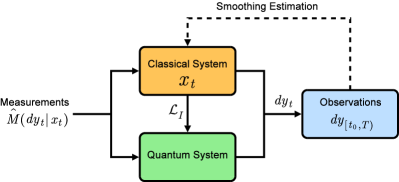
Figure 3: (Color online). Schematic of the hybrid classical-quantum smoothing problem.

Consider the problem of waveform estimation in a hybrid classical-quantum system depicted in Fig. 3. The classical system produces a vectoral classical diffusive Markov random process $x_{t}$, which obeys Eq. (6) and is coupled to the quantum system. The goal is to estimate $x_{\tau}$ via continuous measurements of both systems. This setup is slightly more general than that considered in tsang_smooth ; here the observations can also depend on $x_{t}$. This allows one to apply the theory to PLL design for squeezed beams, as considered by Berry and Wiseman berry , and potentially to other quantum estimation problems as well was . The statistics of $x_{t}$ are assumed to be unperturbed by the coupling to the quantum system, in order to avoid the nontrivial issue of quantum backaction on classical systems backaction . For simplicity, in this section we neglect the possibility that the system noise driving the classical system is correlated with the observation noise, although the noise driving the quantum system can still be correlated with the observation noise due to quantum measurement backaction. Just as in the classical smoothing problem, the hybrid smoothing problem is solved by calculating the smoothing probability density $P(x_{\tau}|dy_{[t_{0},T)})$.

III.2 Time-symmetric approach

Because a quantum system is involved, one may be tempted to use a hybrid density operator backaction ; tsang_smooth ; berry ; was to represent one’s knowledge about the hybrid classical-quantum system. The hybrid density operator $\hat{\rho}(x_{\tau})$ describes the joint classical and quantum statistics of a hybrid system, with the marginal classical probability density for $x_{\tau}$ and the marginal density operator for the quantum system given by

$$P(x_{\tau}) =\operatorname{tr}\left[\hat{\rho}(x_{\tau})\right],$$ (84)

$$\hat{\rho}(\tau) =\int dx_{\tau}\hat{\rho}(x_{\tau}),$$ (85)

respectively. The hybrid operator can also be regarded as a special case of the quantum density operator, when certain degrees of freedom are approximated as classical. Unfortunately, the density operator in conventional predictive quantum theory can only be conditioned upon past observations and not future ones, so it cannot be used as a quantum version of the smoothing probability density.

The classical time-symmetric smoothing theory, as a combination of prediction and retrodiction, offers an important clue to how one can circumvent the difficulty of defining the smoothing quantum state. Again casting the problem in discrete time, and defining a hybrid effect operator as $\hat{E}(\delta y_{\textrm{future}}|x_{\tau})$, which can be used to determine the statistics of future observations given a density operator at $\tau$,

$$P(\delta y_{\textrm{future}}) =\int dx_{\tau}\operatorname{tr}\left[\hat{E}(\delta y_{\textrm{future}}|x_{\tau})\hat{\rho}(x_{\tau})\right],$$ (86)

one may write, in analogy with Eq. (38) tsang_smooth ,

$$P(x_{\tau}|\delta y_{[t_{0},T-\delta t]}) =\frac{P(x_{\tau},\delta y_{\textrm{future}}|\delta y_{\textrm{past}})}{P(\delta y_{\textrm{future}}|\delta y_{\textrm{past}})}$$

$$=\frac{\operatorname{tr}[\hat{E}(\delta y_{\textrm{future}}|x_{\tau})\hat{\rho}(x_{\tau}|\delta y_{\textrm{past}})]}{\int dx_{\tau}\operatorname{tr}[\hat{E}(\delta y_{\textrm{future}}|x_{\tau})\hat{\rho}(x_{\tau}|\delta y_{\textrm{past}})]},$$ (87)

where $\hat{\rho}(x_{\tau}|\delta y_{\textrm{past}})$ is the analog of the filtering probability density $P(x_{\tau}|\delta y_{\textrm{past}})$ and $\hat{E}(\delta y_{\textrm{future}}|x_{\tau})$ is the analog of the retrodictive likelihood function $P(\delta y_{\textrm{future}}|x_{\tau})$. One can then solve for the density and effect operators separately, before combining them to form the classical smoothing probability density.

III.3 Filtering

Since the hybrid density operator can be regarded as a special case of the density operator, the same tools in quantum measurement theory can be used to derive a filtering equation for the hybrid operator. First, write $\hat{\rho}(x_{t+\delta t}|\delta y_{[t_{0},t]})$ in terms of $\hat{\rho}(x_{t}|\delta y_{[t_{0},t]})$ as

$$\hat{\rho}(x_{t+\delta t}|\delta y_{[t_{0},t]}) =\int dx_{t}\mathcal{K}(x_{t+\delta t}|x_{t})\hat{\rho}(x_{t}|\delta y_{[t_{0},t]}),$$ (88)

where $\mathcal{K}$ is a completely positive map that governs the Markovian evolution of the hybrid state independent of the measurement process. Equation (88) may be regarded as a quantum version of the classical Chapman-Kolmogorov equation. For infinitesimal $\delta t$,

$$\int dx_{t}\mathcal{K}(x_{t+\delta t}|x_{t})\hat{\rho}(x_{t}) \approx\left[\left(\hat{1}+\delta t\mathcal{L}\right)\hat{\rho}(x_{t}=x)\right]_{x=x_{t+\delta t}}.$$ (89)

The hybrid superoperator $\mathcal{L}$ can be expressed as

$$\mathcal{L}\hat{\rho}(x) =\mathcal{L}_{0}\hat{\rho}(x)+\mathcal{L}_{I}(x)\hat{\rho}(x)-\sum_{\mu}\frac{\partial}{\partial x_{\mu}}\left[A_{\mu}\hat{\rho}(x)\right]$$

$$\quad+\frac{1}{2}\sum_{\mu,\nu}\frac{\partial^{2}}{\partial x_{\mu}\partial x_{\nu}}\left[\left(BQB^{T}\right)_{\mu\nu}\hat{\rho}(x)\right],$$ (90)

where $\mathcal{L}_{0}$ governs the evolution of the quantum system, $\mathcal{L}_{I}$ governs the coupling of $x_{t}$ to the quantum system, via an interaction Hamiltonian for example, and the last two terms governs the classical evolution of $x_{t}$.

Next, write $\hat{\rho}(x_{t}|\delta y_{[t_{0},t]})$ in terms of $\hat{\rho}(x_{t}|\delta y_{[t_{0},t-\delta t]})$ using the quantum Bayes theorem gardiner_zoller as

$$\hat{\rho}(x_{t}|\delta y_{[t_{0},t]}) =\hat{\rho}(x_{t}|\delta y_{[t_{0},t-\delta t]},\delta y_{t})$$

$$=\frac{\mathcal{J}(\delta y_{t}|x_{t})\hat{\rho}(x_{t}|\delta y_{[t_{0},t-\delta t]})}{\int dx_{t}\operatorname{tr}(\textrm{numerator})}.$$ (91)

The measurement superoperator $\mathcal{J}(\delta y_{t}|x_{t})$, a quantum version of $P(\delta y_{t}|x_{t})$, is defined as

$$\mathcal{J}(\delta y_{t}|x_{t})\hat{\rho}(x_{t}) \equiv\hat{M}(\delta y_{t}|x_{t})\hat{\rho}(x_{t})\hat{M}^{\dagger}(\delta y_{t}|x_{t}).$$ (92)

For infinitesimal $\delta t$ and measurements with Gaussian noise, the measurement operator $\hat{M}$ can be approximated as diosi

$$\hat{M}(\delta z_{t}|x_{t}) \propto\hat{1}+\sum_{\mu}\gamma_{\mu}(t)\bigg{[}\frac{1}{2}\hat{c}_{\mu}(x_{t},t)\delta z_{\mu t}$$

$$\quad-\frac{\delta t}{8}\hat{c}^{\dagger}_{\mu}(x_{t},t)\hat{c}_{\mu}(x_{t},t)\bigg{]},$$ (93)

where $\delta z_{t}$ is a vectoral observation process, $\hat{c}(x_{t},t)$ is a vector of hybrid operators, generalized from the purely quantum $\hat{c}$ operators in Ref. tsang_smooth so that the observations may also depend directly on the classical degrees of freedom, and $\gamma_{\mu}(t)$ is assumed to be positive. To cast the theory in a form similar to the classical one, perform unitary transformations on $\delta z_{t}$ and $\hat{c}$,

$$\delta y_{t} =U\delta z_{t},$$ (94)

$$\hat{C}(x_{t},t) =U\hat{c}(x_{t},t),$$ (95)

where $U$ is a unitary matrix, and rewrite the measurement operator as

$$\hat{M}(\delta y_{t}|x_{t}) \propto\hat{1}+\frac{1}{2}\hat{C}^{T}(x_{t},t)R^{-1}(t)\delta y_{t}$$

$$\quad-\frac{\delta t}{8}\hat{C}^{\dagger T}(x_{t},t)R^{-1}(t)\hat{C}(x_{t},t).$$ (96)

$\hat{C}(x_{t},t)$ is a generalization of $C(x_{t},t)$ in the classical case, and $R(t)$ is again a positive-definite matrix that characterizes the observation uncertainties and is real and symmetric with eigenvalues $1/\gamma_{\mu}$. Note that ^† is defined as the adjoint of each vector element, and ^T is defined as the matrix transpose of the vector. For example,

$$\hat{C}^{\dagger T}R^{-1}\hat{C}\equiv\sum_{\mu,\nu}\hat{C}_{\mu}^{\dagger}(R^{-1})_{\mu\nu}\hat{C}_{\nu}.$$ (97)

The evolution of $\hat{\rho}(x_{t}|\delta y_{[t_{0},t-\delta t]})$ can thus be calculated by iterating the formula

$$\quad\hat{\rho}(x_{t+\delta t}|\delta y_{[t_{0},t]})$$

$$=\int dx_{t}\mathcal{K}(x_{t+\delta t}|x_{t})\frac{\mathcal{J}(\delta y_{t}|x_{t})\hat{\rho}(x_{t}|\delta y_{[t_{0},t-\delta t]})}{\int dx_{t}\operatorname{tr}(\textrm{numerator})}.$$ (98)

Taking the continuous time limit via Itō calculus and defining the conditional hybrid density operator at time $t$ as

$$\hat{F}(x,t) \equiv\hat{\rho}(x_{t}=x|dy_{[t_{0},t)}),$$ (99)

one obtains tsang_smooth

$$d\hat{F} =dt\mathcal{L}\hat{F}$$

$$\quad+\frac{dt}{8}\left(2\hat{C}^{T}R^{-1}\hat{F}\hat{C}^{\dagger}-\hat{C}^{\dagger T}R^{-1}\hat{C}\hat{F}-\hat{F}\hat{C}^{\dagger T}R^{-1}\hat{C}\right)$$

$$\quad+\frac{1}{2}\left[\left(\hat{C}-\langle\hat{C}\rangle_{\hat{F}}\right)^{T}R^{-1}d\eta_{t}\hat{F}+\textrm{H.c.}\right],$$ (100)

where

$$\langle\hat{C}\rangle_{\hat{F}} \equiv\int dx\operatorname{tr}\left[\hat{C}(x,t)\hat{F}(x,t)\right],$$ (101)

$$d\eta_{t} \equiv dy_{t}-\frac{dt}{2}\langle\hat{C}+\hat{C}^{\dagger}\rangle_{\hat{F}}$$ (102)

is a Wiener increment with covariance matrix $R(t)dt$ diosi , H.c. denotes the Hermitian conjugate, and the initial condition is the a priori hybrid density operator $\hat{\rho}(x_{t_{0}})$. Equation (100) is a quantum version of the KS equation (47) and can be regarded as a special case of the Belavkin quantum filtering equation belavkin .

A linear version of the KS equation for an unnormalized $\hat{F}(x,t)$ is

$$d\hat{f} =dt\mathcal{L}\hat{f}$$

$$\quad+\frac{dt}{8}\left(2\hat{C}^{T}R^{-1}\hat{f}\hat{C}^{\dagger}-\hat{C}^{\dagger T}R^{-1}\hat{C}\hat{f}-\hat{f}\hat{C}^{\dagger T}R^{-1}\hat{C}\right)$$

$$\quad+\frac{1}{2}\left(\hat{C}^{T}R^{-1}dy_{t}\hat{f}+\textrm{H.c.}\right),$$ (103)

and the normalization is

$$\hat{F}(x,t) =\frac{\hat{f}(x,t)}{\int dx\operatorname{tr}[\hat{f}(x,t)]}.$$ (104)

Equation (103) is a quantum generalization of the DMZ equation (52).

III.4 Retrodiction and smoothing

Taking a similar approach to the one in Sec. II.4 and using the quantum regression theorem, one can express the future observation statistics as carmichael

$$P(\delta y_{\textrm{future}}) =\int dx_{\tau}\operatorname{tr}\left[\hat{E}(\delta y_{\textrm{future}}|x_{\tau})\hat{\rho}(x_{\tau})\right]$$ (105)

$$=\int dx_{T}\operatorname{tr}\bigg{[}\int dx_{T-\delta t}\mathcal{K}(x_{T}|x_{T-\delta t})$$

$$\quad\cdot\mathcal{J}(\delta y_{T-\delta t}|x_{T-\delta t})$$

$$\quad\cdot\int dx_{T-2\delta t}\mathcal{K}(x_{T-\delta t}|x_{T-2\delta t})$$

$$\quad\cdot\mathcal{J}(\delta y_{T-2\delta t}|x_{T-2\delta t})\dots$$

$$\quad\cdot\int dx_{\tau}\mathcal{K}(x_{\tau+\delta t}|x_{\tau})\mathcal{J}(\delta y_{\tau}|x_{\tau})\hat{\rho}(x_{\tau})\bigg{]},$$ (106)

which are analogous to Eq. (54) and Eq. (62), respectively. Comparing Eq. (105) with Eq. (106), and defining the adjoint of a superoperator $\mathcal{O}$ as $\mathcal{O}^{*}$, such that

$$\operatorname{tr}\left[\hat{E}(x)\mathcal{O}\hat{\rho}(x)\right] =\operatorname{tr}\left\{\left[\mathcal{O}^{*}\hat{E}(x)\right]\hat{\rho}(x)\right\},$$ (107)

the hybrid effect operator can be written as

$$\quad\hat{E}(\delta y_{\textrm{future}}|x_{\tau})$$

$$=\mathcal{J}^{*}(\delta y_{\tau}|x_{\tau})\int dx_{\tau+\delta t}\mathcal{K}^{*}(x_{\tau+\delta t}|x_{\tau})\dots$$

$$\quad\cdot\mathcal{J}^{*}(\delta y_{T-2\delta t}|x_{T-2\delta t})\int dx_{T-\delta t}\mathcal{K}^{*}(x_{T-\delta t}|x_{T-2\delta t})$$

$$\quad\cdot\mathcal{J}^{*}(\delta y_{T-\delta t}|x_{T-\delta t})\int dx_{T}\mathcal{K}^{*}(x_{T}|x_{T-\delta t})\hat{1}.$$ (108)

The operation $\mathcal{K}^{*}\equiv\int dx^{\prime}\mathcal{K}^{*}(x^{\prime}|x)\cdot$ may also be regarded as a hybrid superoperator on a hybrid operator, and is the adjoint of $\mathcal{K}\equiv\int dx^{\prime}\mathcal{K}(x|x^{\prime})\cdot$, defined by

$$\left\langle\hat{E}(x),\mathcal{K}\hat{\rho}(x)\right\rangle =\left\langle\mathcal{K}^{*}\hat{E}(x),\hat{\rho}(x)\right\rangle,$$ (109)

with respect to the Hilbert-Schmidt inner product

$$\left\langle\hat{E}(x),\hat{\rho}(x)\right\rangle \equiv\int dx\operatorname{tr}\left[\hat{E}(x)\hat{\rho}(x)\right].$$ (110)

One can then rewrite Eqs. (105), (106), and (108) more elegantly as

$$\left\langle\hat{E}(x),\hat{\rho}(x)\right\rangle =\left\langle\hat{1},\mathcal{K}\mathcal{J}\dots\mathcal{K}\mathcal{J}\hat{\rho}(x)\right\rangle,$$ (111)

$$\hat{E}(x) =\mathcal{J}^{*}\mathcal{K}^{*}\dots\mathcal{J}^{*}\mathcal{K}^{*}\hat{1}.$$ (112)

In the continuous time limit, a linear stochastic differential equation for the unnormalized effect operator $\hat{g}(x,t)\propto\hat{E}(dy_{[t,T)}|x_{t}=x)$ can be derived. The result is tsang_smooth

$$-d\hat{g} =dt\mathcal{L}^{*}\hat{g}$$

$$\quad+\frac{dt}{8}\left(2\hat{C}^{\dagger T}R^{-1}\hat{g}\hat{C}-\hat{g}\hat{C}^{\dagger T}R^{-1}\hat{C}-\hat{C}^{\dagger T}R^{-1}\hat{C}\hat{g}\right)$$

$$\quad+\frac{1}{2}\left(\hat{g}\hat{C}^{T}R^{-1}dy_{t}+\textrm{H.c.}\right),$$ (113)

to be solved backward in time in the backward Itō sense, with the final condition

$$\hat{g}(x,t)\propto\hat{1}.$$ (114)

Equation (113) is the adjoint equation of the forward quantum DMZ equation (103) with respect to the inner product defined by Eq. (110). It is a generalization of the classical backward DMZ equation (65).

Finally, after solving Eq. (103) for $\hat{f}(x,\tau)$ and Eq. (113) for $\hat{g}(x,\tau)$, the smoothing probability density is

$$h(x,\tau) \equiv P(x_{\tau}=x|dy_{[t_{0},T)})=\frac{\operatorname{tr}[\hat{g}(x,\tau)\hat{f}(x,\tau)]}{\int dx\operatorname{tr}[\hat{g}(x,\tau)\hat{f}(x,\tau)]}.$$ (115)

The denominator of Eq. (115) ensures that $h(x,\tau)$ is normalized, so $\hat{f}(x,\tau)$ and $\hat{g}(x,\tau)$ need not be normalized separately. Table 1 lists some important quantities in classical smoothing with their generalizations in hybrid smoothing for comparison.

Classical	Description	Hybrid	Description
$P(x_{t+\delta t}|x_{t},\delta y_{t})$	transition probability density, appears in Chapman-Kolmogorov equation (40)	$\mathcal{K}(x_{t+\delta t}|x_{t})$	transition superoperator, appears in quantum Chapman-Kolmogorov equation (88)
$P(\delta y_{t}|x_{t})$	observation probability density, appears in Bayes theorem (43)	$\mathcal{J}(\delta y_{t}|x_{t})$	measurement superoperator, appears in quantum Bayes theorem (91)
$P(x_{t}|dy_{[t_{0},t)})$, $F(x,t)$	filtering probability density, obeys Kushner-Stratonovich equation (47)	$\hat{\rho}(x_{t}|dy_{[t_{0},t)})$, $\hat{F}(x,t)$	filtering hybrid density operator, obeys Belavkin equation (100)
$f(x,t)$	unnormalized $F(x,t)$, obeys Duncan-Mortensen-Zakai (DMZ) equation (52)	$\hat{f}(x,t)$	unnormalized $f(x,t)$, obeys quantum DMZ equation (103)
$P(dy_{[t,T)}|x_{t})$	retrodictive likelihood function	$\hat{E}(dy_{[t,T)}|x_{t})$	hybrid effect operator
$g(x,t)$	unnormalized $P(dy_{[t,T)}|x_{t})$, obeys backward DMZ equation (65)	$\hat{g}(x,t)$	unnormalized $\hat{E}(dy_{[t,T)}|x_{t})$, obeys backward quantum DMZ equation (113)
$P(x_{\tau}|dy_{[t_{0},T)})$, $h(x,\tau)$	smoothing probability density, obeys Eq. (72)	$P(x_{\tau}|dy_{[t_{0},T)})$, $h(x,\tau)$	smoothing probability density, obeys Eq. (115)

Table 1: Important quantities in classical smoothing and their generalizations in hybrid smoothing.

III.5 Smoothing in terms of Wigner distributions

To solve Eqs. (103), (113), and (115), one way is to convert them to equations for quasiprobability distributions walls . The Wigner distribution is especially useful for quantum systems with continuous degrees of freedom. It is defined as walls ; mandel

$$f(q,p) \equiv\frac{1}{2\pi}\int du\left\langle q-\frac{u}{2}\right|\hat{f}\left|q+\frac{u}{2}\right\rangle\exp\left(ip^{T}u\right),$$ (116)

where $q$ and $p$ are normalized position and momentum vectors. It has the desirable property

$$\int dqdpg(q,p)f(q,p) =\frac{1}{2\pi}\operatorname{tr}\left(\hat{g}\hat{f}\right),$$ (117)

which is unique among generalized quasiprobability distributions mandel . The smoothing probability density given by Eq. (115) can then be rewritten as

$$h(x,\tau) =\frac{\int dqdpg(q,p,x,\tau)f(q,p,x,\tau)}{\int dqdpdxg(q,p,x,\tau)f(q,p,x,\tau)},$$ (118)

where $f(q,p,x,\tau)$ and $g(q,p,x,\tau)$ are the Wigner distributions of $\hat{f}$ and $\hat{g}$, respectively. Equation (118) resembles the classical expression (72) with the quantum degrees of freedom $q$ and $p$ marginalized. If $f(q,p,x,t_{0})$ is nonnegative and the stochastic equations for $f(q,p,x,t)$ and $g(q,p,x,t)$ converted from Eqs. (103) and (113) have the same form as the classical DMZ equations given by Eqs. (52) and (65), the hybrid smoothing problem becomes equivalent to a classical one and can be solved using well known classical smoothers. For example, if $f(q,p,x,t)$ and $g(q,p,x,t)$ are Gaussian, $h(x,\tau)$ is also Gaussian, and their means and covariances can be solved using the linear MFP smoother described in Sec. II.5.

IV Phase-locked loop design for narrowband squeezed beams

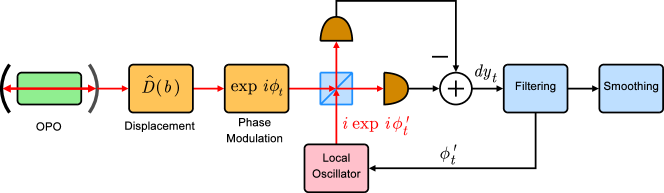
Figure 4: (Color online). Homodyne phase-locked loop (PLL) for phase estimation with a narrowband squeezed optical beam produced from an optical parametric oscillator (OPO).

Consider the PLL setup depicted in Fig. 4. The optical parametric oscillator (OPO) produces a squeezed vacuum with a squeezed $p$ quadrature and an antisqueezed $q$ quadrature. The squeezed vacuum is then displaced by a real constant $b$ to produce a phase-squeezed beam, the phase of which is modulated by $\phi_{t}=x_{1t}$, an element of the vectoral random process $x_{t}$ described by the system Itō equation (6). The output beam is measured continuously by a homodyne PLL, and the local-oscillator phase $\phi_{t}^{\prime}$ is continuously updated according to the real-time measurement record.

The use of PLL for phase estimation in the presence of quantum noise has been mentioned as far back as 1971 by Personick personick . Wiseman suggested an adaptive homodyne scheme to measure a constant phase wiseman , which was then experimentally demonstrated by Armen et al. for the optical coherent state armen . Berry and Wiseman berry1 and Pope et al. pope studied the problem with $\phi_{t}$ being a Wiener process. Berry and Wiseman later generalized the theory to account for narrowband squeezed beams berry . Tsang et al. also studied the problem for the case of $x_{t}$ being a Gaussian process tsang ; tsang2 , but the squeezing model considered in Refs. tsang ; tsang2 is not realistic. Using the hybrid smoothing theory developed in Sec. III, one can now generalize these earlier results to the case of an arbitrary diffusive Markov process and a realistic squeezing model.

Let $\hat{\rho}(x_{t})$ be the hybrid density operator for the combined quantum-OPO-classical-modulator system. The evolution of the OPO below threshold in the interaction picture is governed by

$$\mathcal{L}_{0}\hat{\rho}(x) =-\frac{i}{\hbar}\left[\hat{H}_{0},\hat{\rho}(x)\right],$$ (119)

$$\hat{H}_{0} =-i\frac{\hbar\chi}{2}\left(\hat{a}\hat{a}-\hat{a}^{\dagger}\hat{a}^{\dagger}\right)$$ (120)

$$=\frac{\hbar\chi}{2}\left(\hat{q}\hat{p}+\hat{p}\hat{q}\right),$$ (121)

where $\hat{a}$ is the annihilation operator for the cavity optical mode, and $\hat{q}$ and $\hat{p}$ are the antisqueezed and squeezed quadrature operators, respectively, defined as

$$\hat{q} \equiv\frac{\hat{a}+\hat{a}^{\dagger}}{\sqrt{2}},$$ (122)

$$\hat{p} \equiv\frac{\hat{a}-\hat{a}^{\dagger}}{\sqrt{2}i},$$ (123)

with the commutation relation

$$[\hat{q},\hat{p}] =i.$$ (124)

The classical phase modulator does not influence the evolution of the OPO, so

$$\mathcal{L}_{I}=0,$$ (125)

but it modulates the OPO output. $\hat{C}(x_{t},t)$ in this case is

$$\hat{C}(x_{t},t) =-2i\left(b+\sqrt{\gamma}\hat{a}\right)\exp\left(i\phi_{t}-i\phi_{t}^{\prime}\right),$$ (126)

where $\gamma$ is the transmission coefficient of the partially reflecting OPO output mirror, $R=1$, and the symbol and sign conventions here roughly follows those of Refs. tsang ; tsang2 . To ensure the correct unconditional quantum dynamics, the Hamiltonian should be changed to (Ref. gardiner_zoller , Sec. 11.4.3)

$$\hat{H}_{0}^{\prime} =\hat{H}_{0}-i\frac{i\hbar b\sqrt{\gamma}}{2}(\hat{a}-\hat{a}^{\dagger}), \mathcal{L}_{0}\hat{\rho}(x) =-\frac{i}{\hbar}\left[\hat{H}_{0}^{\prime},\hat{\rho}(x)\right],$$ (127)

in order to eliminate the spurious effect of the displacement term in $\hat{C}$ on the OPO. After some algebra, the forward stochastic equation for the Wigner distribution $f(q,p,x,t)$ becomes

$$df =dt\bigg{\{}-\sum_{\mu}\frac{\partial}{\partial x_{\mu}}(A_{\mu}f)+\frac{1}{2}\sum_{\mu,\nu}\frac{\partial^{2}}{\partial x_{\mu}\partial x_{\nu}}\left[\left(BQB^{T}\right)_{\mu\nu}f\right]$$

$$\quad-\left[\left(\chi-\frac{\gamma}{2}\right)\frac{\partial}{\partial q}\left(qf\right)+\left(-\chi-\frac{\gamma}{2}\right)\frac{\partial}{\partial p}\left(pf\right)\right]$$

$$\quad+\frac{\gamma}{4}\left(\frac{\partial^{2}f}{\partial q^{2}}+\frac{\partial^{2}f}{\partial p^{2}}\right)\bigg{\}}$$

$$\quad+dy_{t}\bigg{[}\sin(\phi-\phi_{t}^{\prime})\left(2b+\sqrt{2\gamma}q+\sqrt{\frac{\gamma}{2}}\frac{\partial}{\partial q}\right)$$

$$\quad+\cos(\phi-\phi_{t}^{\prime})\left(\sqrt{2\gamma}p+\sqrt{\frac{\gamma}{2}}\frac{\partial}{\partial p}\right)\bigg{]}f.$$ (128)

This is precisely the classical DMZ equation (52) with correlated system and observation noises. The equivalent classical system equations are then

$$dq_{t} =\left(\chi-\frac{\gamma}{2}\right)q_{t}dt+\sqrt{\frac{\gamma}{2}}d\alpha_{t},$$

$$dp_{t} =\left(-\chi-\frac{\gamma}{2}\right)p_{t}dt+\sqrt{\frac{\gamma}{2}}d\beta_{t},$$

$$dx_{t} =A(x_{t},t)dt+B(x_{t},t)dW_{t},$$ (129)

and the equivalent observation equation is

$$dy_{t} =2b\sin(\phi_{t}-\phi_{t}^{\prime})dt+d\zeta_{t},$$

$$d\zeta_{t} \equiv\sin(\phi_{t}-\phi_{t}^{\prime})\left(\sqrt{2\gamma}q_{t}dt-d\alpha_{t}\right)$$

$$\quad+\cos(\phi_{t}-\phi_{t}^{\prime})\left(\sqrt{2\gamma}p_{t}dt-d\beta_{t}\right),$$ (130)

where $d\alpha_{t}$ and $d\beta_{t}$ are independent Wiener increments with covariance $dt$. $d\alpha_{t}$ and $d\beta_{t}$, which appear in both the system equation and the observation equation, are simply quadratures of the vacuum field, coupled to both the cavity mode and the output field via the OPO output mirror. Equations (129) and (130) coincide with the model of Berry and Wiseman in Ref. berry when $x_{t}$ is a Wiener process, and Eq. (128) is the continuous limit of their approach to phase estimation. This approach can also be regarded as an example of the general method of accounting for colored observation noise by modeling the noise as part of the system vantrees ; crassidis ; simon .

If $\chi=0$, $d\zeta_{t}/dt$ is an additive white Gaussian noise, and the model is reduced to that studied in Refs. berry1 ; pope ; tsang ; tsang2 . In that case, it is desirable to make $\phi_{t}^{\prime}$ follow $\phi_{t}$ as closely as possible, so that $dy_{t}$ can be approximated as

$$dy_{t} \approx 2b(\phi_{t}-\phi_{t}^{\prime})dt+d\zeta_{t},$$ (131)

and the Kalman filter can be used if $x_{t}$ is Gaussian tsang2 . Provided that Eq. (131) is valid, one should make $\phi_{t}^{\prime}$ the conditional expectation of $\phi_{t}=x_{1t}$, given by

$$\phi_{t}^{\prime} =\left\langle\phi_{t}\right\rangle_{\hat{f}}=\int dqdpdx\,x_{1}f(q,p,x,t).$$ (132)

For phase-squeezed beams, it also seems desirable to make $\phi_{t}^{\prime}$ close to $\phi_{t}$ in order to minimize the magnitude of $d\zeta_{t}$. Equation (132) may not provide the optimal $\phi_{t}^{\prime}$ in general, however, as it does not necessarily minimize the magnitude of $d\zeta_{t}$ or the estimation errors. The optimal control law for $\phi_{t}^{\prime}$ should be studied in the context of control theory.

While $\phi_{t}^{\prime}$ needs to be updated in real time and must be calculated via filtering, the estimation accuracy can be improved by smoothing. The backward DMZ equation for $g(q,p,x,t)$ is the adjoint equation with respect to Eq. (128), given by

$$-dg =dt\bigg{\{}\sum_{\mu}A_{\mu}\frac{\partial g}{\partial x_{\mu}}+\frac{1}{2}\sum_{\mu,\nu}\left(BQB^{T}\right)_{\mu\nu}\frac{\partial^{2}g}{\partial x_{\mu}\partial x_{\nu}}$$

$$\quad+\left[\left(\chi-\frac{\gamma}{2}\right)q\frac{\partial g}{\partial q}+\left(-\chi-\frac{\gamma}{2}\right)p\frac{\partial g}{\partial p}\right]$$

$$\quad+\frac{\gamma}{4}\left(\frac{\partial^{2}g}{\partial q^{2}}+\frac{\partial^{2}g}{\partial p^{2}}\right)\bigg{\}}$$

$$\quad+dy_{t}\bigg{[}\sin(\phi-\phi_{t}^{\prime})\left(2b+\sqrt{2\gamma}q-\sqrt{\frac{\gamma}{2}}\frac{\partial}{\partial q}\right)$$

$$\quad+\cos(\phi-\phi_{t}^{\prime})\left(\sqrt{2\gamma}p-\sqrt{\frac{\gamma}{2}}\frac{\partial}{\partial p}\right)\bigg{]}g,$$ (133)

and the smoothing probability density $h(x,\tau)$ is given by Eq. (118). The use of linear smoothing for the case of $x_{t}$ being a Gaussian process and $d\zeta_{t}/dt$ being a white Gaussian noise has been studied in Refs. tsang ; tsang2 . Practical strategies of solving Eqs. (128) and (133) in general are beyond the scope of this paper, but classical nonlinear filtering and smoothing techniques should help jazwinski ; vantrees ; crassidis ; simon .

One can also use the hybrid smoothing theory to study the general problem of force estimation via a squeezed probe beam and a homodyne PLL, by modeling the phase modulator as a quantum mechanical oscillator instead and combining the problem studied in this section with the force estimation problem studied in Ref. tsang_smooth .

V Weak values as quantum smoothing estimates

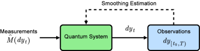
Figure 5: (Color online). The quantum smoothing problem.

Previous sections focus on the estimation of classical signals, but there is no reason why one cannot apply smoothing to quantum degrees of freedom as well, as shown in Fig. 5. First consider the predicted density operator at time $\tau$ conditioned upon past observations, given by

$$\hat{\rho}(\tau) \equiv\frac{\hat{f}(\tau)}{\operatorname{tr}[\hat{f}(\tau)]},$$ (134)

where the classical degrees of freedom are neglected for simplicity. The predicted expectation of an observable, such as the position of a quantum mechanical oscillator, is

$$\langle\hat{O}\rangle_{\hat{f}} \equiv\operatorname{tr}\left[\hat{O}\hat{\rho}(\tau)\right]=\frac{\operatorname{tr}[\hat{O}\hat{f}(\tau)]}{\operatorname{tr}[\hat{f}(\tau)]}.$$ (135)

One may also use retrodiction, after some measurements of a quantum system have been made, to estimate its initial quantum state before the measurements barnett ; yanagisawa , using the retrodictive density operator defined as

$$\hat{\rho}_{\textrm{ret}}(\tau) \equiv\frac{\hat{g}(\tau)}{\operatorname{tr}[\hat{g}(\tau)]}.$$ (136)

The retrodicted expectation of an observable is

$${}_{\hat{g}}\langle\hat{O}\rangle \equiv\operatorname{tr}\left[\hat{\rho}_{\textrm{ret}}(\tau)\hat{O}\right]=\frac{\operatorname{tr}[\hat{g}(\tau)\hat{O}]}{\operatorname{tr}[\hat{g}(\tau)]}.$$ (137)

Causality prevents one from going back in time to verify the retrodicted expectation, but if the degree of freedom with respect to $\hat{O}$ at time $\tau$ is entangled with another “probe” system, then one can verify the retrodicted expectation by measuring the probe and inferring $\hat{O}$ yanagisawa .

The idea of verifying retrodiction by entangling the system at time $\tau$ with a probe can also be extended to the case of smoothing, as proposed by Aharonov et al. aav . In the middle of a sequence of measurements, if one weakly couples the system to a probe for a short time, so that the system is weakly entangled with the probe, and the probe is subsequently measured, the measurement outcome on average can be characterized by the so-called weak value of an observable, defined as aav ; wiseman_aav

$${}_{\hat{g}}\langle\hat{O}\rangle_{\hat{f}} \equiv\frac{\operatorname{tr}[\hat{g}(\tau)\hat{O}\hat{f}(\tau)]}{\operatorname{tr}[\hat{g}(\tau)\hat{f}(\tau)]}.$$ (138)

The weak value becomes a prediction given by Eq. (135) when future observations are neglected, such that $\hat{g}(\tau)=\hat{1}$, and becomes a retrodiction given by Eq. (137) when past observations are neglected and there is no a priori information about the quantum system at time $\tau$, such that $\hat{f}(\tau)=\hat{1}$. When $\hat{f}(\tau)$ and $\hat{g}(\tau)$ are incoherent mixtures of $\hat{O}$ eigenstates,

$$\hat{f}(\tau) =\sum_{O}f(O,\tau)|O\rangle\langle O|,$$ (139)

$$\hat{g}(\tau) =\sum_{O}g(O,\tau)|O\rangle\langle O|,$$ (140)

the weak value becomes

$${}_{\hat{g}}\langle\hat{O}\rangle_{\hat{f}} =\frac{\sum_{O}Og(O,\tau)f(O,\tau)}{\sum_{O}g(O,\tau)f(O,\tau)},$$ (141)

and is consistent with the classical time-symmetric smoothing theory described in Sec. II. Hence, the weak value can be regarded as a quantum generalization of the smoothing estimate, conditioned upon past and future observations.

One can also establish a correspondence between a classical theory and a quantum theory via quasiprobability distributions. Given the smoothing probability density in terms of the Wigner distributions in Eq. (118), one may be tempted to undo the marginalizations over the quantum degrees of freedom and define a smoothing quasiprobability distribution as

$$h(q,p,\tau) =\frac{g(q,p,\tau)f(q,p,\tau)}{\int dqdpg(q,p,\tau)f(q,p,\tau)},$$ (142)

where $f(q,p,\tau)$ and $g(q,p,\tau)$ are the Wigner distributions of $\hat{f}(\tau)$ and $\hat{g}(\tau)$, respectively. Intriguingly, $h(q,p,\tau)$, being the product of two Wigner distributions, can exhibit quantum position and momentum uncertainties that violate the Heisenberg uncertainty principle. This has been shown in Ref. tsang2 , when the position of a quantum mechanical oscillator is monitored via continuous measurements and smoothing is applied to the observations. From the perspective of classical estimation theory, it is perhaps not surprising that smoothing can improve upon an uncertainty relation based on a predictive theory. The important question is whether the sub-Heisenberg uncertainties can be verified experimentally. Ref. tsang2 argues that it can be done only by Bayesian estimation, but in the following I shall propose another method based on weak measurements.

It can be shown that the expectation of $q$ using $h(q,p,\tau)$ is

$$\langle q\rangle_{h} \equiv\int dqdp\,qh(q,p,\tau)$$ (143)

$$=\operatorname{Re}\frac{\operatorname{tr}[\hat{g}(\tau)\hat{q}\hat{f}(\tau)]}{\operatorname{tr}[\hat{g}(\tau)\hat{f}(\tau)]}=\operatorname{Re}{}_{\hat{g}}\langle\hat{q}\rangle_{\hat{f}},$$ (144)

which is the real part of the weak value, and likewise for $\langle p\rangle_{h}$, so the smoothing position and momentum estimates are closely related to their weak values. More generally, consider the joint probability density for a quantum position measurement followed by a quantum momentum measurement, conditioned upon past and future observations:

$$P(y_{q},y_{p}) =\frac{1}{\mathcal{C}}\operatorname{tr}\left[\hat{g}(\tau)\hat{M}_{p}(y_{p})\hat{M}_{q}(y_{q})\hat{f}(\tau)\hat{M}_{q}^{\dagger}(y_{q})\hat{M}_{p}^{\dagger}(y_{p})\right],$$ (145)

$$\mathcal{C} \equiv\int dy_{q}dy_{p}\operatorname{tr}\Big{[}\hat{g}(\tau)\hat{M}_{p}(y_{p})\hat{M}_{q}(y_{q})$$

$$\quad\times\hat{f}(\tau)\hat{M}_{q}^{\dagger}(y_{q})\hat{M}_{p}^{\dagger}(y_{p})\Big{]},$$ (146)

where the measurement operators

$$\hat{M}_{q}(y_{q}) =\int dq\left(\frac{\epsilon_{q}}{2\pi}\right)^{\frac{1}{4}}\exp\left[-\frac{\epsilon_{q}}{4}(y_{q}-q)^{2}\right]|q\rangle\langle q|,$$ (147)

$$\hat{M}_{p}(y_{p}) =\int dp\left(\frac{\epsilon_{p}}{2\pi}\right)^{\frac{1}{4}}\exp\left[-\frac{\epsilon_{p}}{4}(y_{p}-p)^{2}\right]|p\rangle\langle p|$$ (148)

are assumed to be Gaussian and backaction evading. After some algebra,

$$P(y_{q},y_{p}) =\int dqdp\left(\frac{\epsilon_{q}}{2\pi}\right)^{\frac{1}{2}}\left(\frac{\epsilon_{p}}{2\pi}\right)^{\frac{1}{2}}$$

$$\quad\times\exp\left[-\frac{\epsilon_{q}}{2}(y_{q}-q)^{2}-\frac{\epsilon_{p}}{2}(y_{p}-p)^{2}\right]\tilde{P}(q,p),$$ (149)

$$\tilde{P}(q,p) \equiv\frac{1}{2\pi\mathcal{C}}\int dudv\exp\left(-\frac{\epsilon_{q}u^{2}+\epsilon_{p}v^{2}}{8}\right)$$

$$\quad\times\left\langle p+\frac{v}{2}\right|\hat{g}(\tau)\left|p-\frac{v}{2}\right\rangle\exp(ivq)$$

$$\quad\times\left\langle q-\frac{u}{2}\right|\hat{f}(\tau)\left|q+\frac{u}{2}\right\rangle\exp(ipu).$$ (150)

From the perspective of classical probability theory, Eq. (149) can be interpreted as the probability density of noisy position and momentum measurements with noise variances $1/\epsilon_{q}$ and $1/\epsilon_{p}$, when the measured object has a classical phase-space density given by $\tilde{P}(q,p)$. In the limit of infinitesimally weak measurements, $\epsilon_{q},\epsilon_{p}\to 0$, and

$$\lim_{\epsilon_{q},\epsilon_{p}\to 0}\tilde{P}(q,p) =h(q,p,\tau).$$ (151)

Thus, $h(q,p,\tau)$ can be obtained approximately from an experiment with small $\epsilon_{q}$ and $\epsilon_{p}$ by measuring $P(y_{q},y_{p})$ for the same $\hat{g}$ and $\hat{f}$ and deconvolving Eq. (149). In practice, $\epsilon_{q}$ and $\epsilon_{p}$ only need to be small enough such that $\tilde{P}(q,p)\approx h(q,p,\tau)$. This allows one, at least in principle, to experimentally demonstrate the sub-Heisenberg uncertainties predicted in Ref. tsang2 in a frequentist way, not just by Bayesian estimation as described in Ref. tsang2 . Note, however, that $h(q,p,\tau)$ can still go negative, so it cannot always be regarded as a classical probability density. This underlines the wave nature of a quantum object and may be related to the negative probabilities encountered in the use of weak values to explain Hardy’s paradox aav_hardy .

VI Conclusion

In conclusion, I have used a discrete-time approach to derive the classical and quantum theories of time-symmetric smoothing. The hybrid smoothing theory is applied to the design of PLL, and the relation between the proposed theory and Aharonov et al.’s weak value theory is discussed. Possible generalizations of the theory include taking jumps into account for the classical random process gardiner and adding quantum measurements with Poisson statistics, such as photon counting gardiner_zoller ; carmichael ; walls ; mandel . Potential applications not discussed in this paper include cavity quantum electrodynamics gardiner_zoller ; carmichael ; walls ; mandel , photodetection theory was ; gardiner_zoller ; mandel , atomic magnetometry budker , and quantum information processing in general. On a more fundamental level, it might also be interesting to generalize the weak value theory and the smoothing quasiprobability distribution to other kinds of quantum degrees of freedom in addition to position and momentum, such as spin, photon number, and phase. A general quantum smoothing theory would complete the correspondence between classical and quantum estimation theories.

References

- (1) A. H. Jazwinski, Stochastic Processes and Filtering Theory (Academic Press, New York, 1970).
- (2) J. C. Crassidis and J. L. Junkins, Optimal Estimation of Dynamic Systems (Chapman & Hall CRC, Boca Raton, 2004).
- (3) H. L. Van Trees, Detection, Estimation, and Modulation Theory, Part I (Wiley, New York, 2001); Detection, Estimation, and Modulation Theory, Part II: Nonlinear Modulation Theory (Wiley, New York, 2002); Detection, Estimation, and Modulation Theory, Part III: Radar-Sonar Processing and Gaussian Signals in Noise (Wiley, New York, 2001).
- (4) D. Simon, Optimal State Estimation (Wiley, Hoboken, 2006).
- (5) M. Tsang, Phys. Rev. Lett. 102, 250403 (2009).
- (6) E. Pardoux, Stochastics 6, 193 (1982). See also B. D. O. Anderson and I. B. Rhodes, Stochastics 9, 139 (1983).
- (7) D. W. Berry and H. M. Wiseman, Phys. Rev. A73, 063824 (2006).
- (8) Y. Aharonov, D. Z. Albert, and L. Vaidman, Phys. Rev. Lett. 60, 1351 (1988); Y. Aharonov and L. Vaidman, J. Phys. A 24, 2315 (1991).
- (9) C. W. Gardiner, Handbook of Stochastic Methods (Springer-Verlag, Berlin, 1985).
- (10) R. L. Stratonovich, Theor. Probability Appl. 5, 156 (1960); H. J. Kushner, J. Math. Anal. Appl. 8, 332 (1964); SIAM J. Control 2, 106 (1964).
- (11) M. Fujisaki, G. Kallianpur, and H. Kunita, Osaka J. Math. 9, 19 (1972).
- (12) P. A. Frost and T. IEEE Trans. Auto. Control AC-16, 217 (1971).
- (13) R. E. Mortensen, Ph.D. dissertation, Univ. of California, Berkeley (1966); T. E. Duncan, Ph.D. dissertation, Stanford University (1967); M. Zakai, Z. Wahr. verw. Geb. 11, 230 (1969).
- (14) D. Q. Mayne, Automatica 4, 73 (1966); D. C. Fraser and J. E. Potter, IEEE Trans. Automatic Control 14, 387 (1969).
- (15) J. E. Wall, Jr., A. S. Willsky, and N. R. Sandell Jr., Stochastics 5, 1 (1981).
- (16) P. Warszawski, H. M. Wiseman, and H. Mabuchi, Phys. Rev. A65, 023802 (2002); P. Warszawski and H. M. Wiseman, J. Opt. B: Quant. Semiclass. Opt. 5, 1 (2003); 5, 15 (2003); N. P. Oxtoby, P. Warszawski, H. M. Wiseman, He-Bi Sun and R. E. S. Polkinghorne, Phys. Rev. B71, 165317 (2005).
- (17) I. V. Aleksandrov, Z. Naturforsch. 36A, 902 (1981); W. Boucher and J. Traschen, Phys. Rev. D37, 3522 (1988); L. Diósi, N. Gisin, and W. T. Strunz, Phys. Rev. A61, 022108 (2000).
- (18) C. W. Gardiner and P. Zoller, Quantum Noise (Springer-Verlag, Berlin, 2000).
- (19) H. M. Wiseman and L. Diósi, Chem. Phys. 268, 91 (2001).
- (20) V. P. Belavkin, Radiotech. Elektron. 25, 1445 (1980); V. P. Belavkin, in Information Complexity and Control in Quantum Physics, edited by A. Blaquière, S. Diner, and G. Lochak (Springer, Vienna, 1987), p. 311; V. P. Belavkin, in Stochastic Methods in Mathematics and Physics, edited by R. Gielerak and W. Karwowski (World Scientific, Singapore, 1989), p. 310; V. P. Belavkin, in Modeling and Control of Systems in Engineering, Quantum Mechanics, Economics, and Biosciences, edited by A. Blaquière (Springer, Berlin, 1989), p. 245.
- (21) A. Barchielli, L. Lanz, and G. M. Prosperi, Nuovo Cimento, 72B, 79 (1982); Found. Phys. 13, 779 (1983); H. Carmichael, An Open Systems Approach to Quantum Optics (Springer-Verlag, Berlin, 1993).
- (22) D. F. Walls and G. J. Milburn, Quantum Optics (Springer-Verlag, Berlin, 2008).
- (23) L. Mandel and E. Wolf, Optical Coherence and Quantum Optics (Cambridge University Press, Cambridge, 1995).
- (24) S. D. Personick, IEEE Trans. Inform. Theor. IT-17, 240 (1971).
- (25) H. M. Wiseman, Phys. Rev. Lett. 75, 4587 (1995).
- (26) M. A. Armen, J. K. Au, J. K. Stockton, A. C. Doherty, and H. Mabuchi, Phys. Rev. Lett. 89, 133602 (2002).
- (27) D. W. Berry and H. M. Wiseman, Phys. Rev. A65, 043803 (2002).
- (28) D. T. Pope, H. M. Wiseman, and N. K. Langford, Phys. Rev. A70, 043812 (2004).
- (29) M. Tsang, J. H. Shapiro, and S. Lloyd, Phys. Rev. A78, 053820 (2008).
- (30) M. Tsang, J. H. Shapiro, and S. Lloyd, Phys. Rev. A79, 053843 (2009).
- (31) S. M. Barnett, D. T. Pegg, J. Jeffers, O. Jedrkiewicz, and R. Loudon, Phys. Rev. A62, 022313 (2000); S. M. Barnett, D. T. Pegg, J. Jeffers, and O. Jedrkiewicz, Phys. Rev. Lett. 86, 2455 (2001); D. T. Pegg, S. M. Barnett, and J. Jeffers, Phys. Rev. A66, 022106 (2002).
- (32) M. Yanagisawa, e-print arXiv:0711.3885.
- (33) H. M. Wiseman, Phys. Rev. A65, 032111 (2002).
- (34) Y. Aharonov, A. Botero, S. Popescu, B. Reznik, and J. Tollaksen, Phys. Lett. A 301, 130 (2002).
- (35) D. Budker, W. Gawlik, D. F. Kimball, S. M. Rochester, V. V. Yashchuk, and A. Weis, Rev. Mod. Phys. 74, 1153 (2002); J. M. Geremia, J. K. Stockton, A. C. Doherty, and H. Mabuchi, Phys. Rev. Lett. 91, 250801 (2003).