On the critical behavior of two-dimensional liquid crystals

Abstract

The Lebwohl-Lasher (LL) model is the traditional model used to describe the nematic-isotropic transition of real liquid crystals. In this paper, we develop a numerical study of the temperature behaviour and of finite-size scaling of the two-dimensional (2D) LL-model. We discuss two possible scenarios. In the first one, the 2D LL-model presents a phase transition similar to the topological transition appearing in the 2D XY-model. In the second one, the 2D LL-model does not exhibit any critical transition, but its low temperature behaviour is rather characterized by a crossover from a disordered phase to an ordered phase at zero temperature. We realize and discuss various comparisons with the 2D XY-model and the 2D Heisenberg model. Adding to previous studies of finite-size scaling behaviour of the order parameter and conformal mapping of order parameter profile, we analyze the critical scaling of the probability distribution function, hyperscaling relations and stiffness order parameter and conclude that the second scenario (no critical transition) is the most plausible.

I Introduction

At high temperatures, the natural state of a liquid crystal is the isotropic phase, because all the molecule orientations are equally probable. At low temperatures, an order along a preferred direction may appear, it is the nematic phase. When such a material is cooled at even lower temperatures, other types of ordered phases are likely to appear, the description of which requires realistic potentials (see e.g. reference Zewdie00 ). The transition between the isotropic and the nematic phases generally occurs at a critical temperature. Various experiments on three-dimensional liquid crystals, exhibited a weak first order transition ZhangMouritsenZuckermann92 . However, the corresponding two-dimensional (2D) problem is far from begin that clear. Experimentally, only 2D liquid crystals composed of long rigid interacting rods have been studied.

First, the 2D problem must be defined through the symmetries: there are generally a continuous global symmetry $O(n)$, and a local $Z_{2}$ symmetry. For example, the two most-studied models deal with $O(2)$ (the XY-model), or $O(3)$ (the Heisenberg model) symmetries. The Hamiltonian reads in both cases as:

$${\cal H}=-J\sum_{\langle i,j\rangle}{{\bf S}_{i}\cdot{\bf S}_{j}},$$ (1)

with ${\bf S}_{i}$ a $n$-components spin, of unit length, at the lattice site $i$. The sum runs over all pairs of neighbouring spins of the 2D square lattice and $J>0$ is the spin-spin coupling constant.

According to the Mermin-Wagner-Hohenberg theorem mw ; h ; mermin1 ; mermin ; coleman , the order parameter fluctuations prevent from any spontaneous breakdown of continuous symmetries for 2D systems with short-range interactions. However, this theorem cannot conclude in the case of transitions to a phase with no long range order. An example of such a 2D critical behaviour, which is not a continuous-symmetry breaking, is the 2D XY-model ($O(2)$, Abelian symmetry). This model presents a topological transition characterized by a critical low temperature phase as a plasma of vortices pairs, at temperatures under the Berezinskii-Kosterlitz-Thouless transition temperature, $T_{BKT}$ bere ; kt . At much lower temperatures, the system state is dominated by spin waves. The high temperature phase occurs when the pairs dissociate.

On the other hand, the 2D Heisenberg model ($O(3)$, non-Abelian symmetry) has no transition at any finite temperature (asymptotic freedom) polya ; brez ; amitbook ; izyu . The longitudinal modes of the $O(3)$ model are frozen for the low temperatures, and only the transverse modes are activated, leading essentially to two Gaussian modes. The deep difference between the two models at finite temperatures, is the stability of the vortices. Indeed, the topological transition of the 2D XY-model is the result of the stability of the topological defects, while the “third spin dimension” in the $O(3)$ model, makes the vortices unstable at any finite temperature.

However, the above picture has been questioned recently by the numerical evidences for a possible transition in the 2D Heisenberg model Niedemayer ; PatrasciouSeiler ; Patrasciou ; Aguado . Moreover it has been shown that a quasi long range order (QLRO) phase tesisAna ; bb might appear at very low temperatures in finite systems. Indeed in these numerical works, the thermodynamic limit remains questionable and the analytic approach of bb relies explicitly on the finite size of the lattice.

A model for a regular 2D liquid crystal system was proposed by Lebwohl and Lasher (LL) ll . Based on a lattice version of the mean field theory of Maier and Saupe MaierSaupe59 , the molecules are represented by $n-$component unit vectors and the “spin-spin” interactions are given by the second Legendre polynomial, $P_{2}$ (keeping the local $Z_{2}$ symmetry). The popularity of the LL-model comes from its ability to reproduce the weak first order phase transition observed experimentally between the isotropic and the nematic phases ZhangMouritsenZuckermann92 in the three-dimensional space. Then, the question of possible phase transitions in this model is attractive and has been addressed in numerous studies. tesisAna ; kuzu ; blote ; caracciolo ; FPB ; PFB

In the past twenty years, several numerical evidences pointed out a possible topological transition for the 2D nematic-isotropic phase transition in liquid crystals. The situation is clear in the case of planar rotator models (see e.g. references FPB2 ; BP ), but still controversial for three-component models. In reference FPB2 , we have studied the nematic-isotropic transition of 2D liquid crystals using a $O(2)$ vector model characterized by nonlinear nearest-neighbour spin interactions governed by the fourth Legendre polynomial $P_{4}$. The system has been studied through standard finite-size scaling and conformal rescaling of the density profiles. We also estimated the Binder cumulant Binder as a function of the temperature for different values of system size $L$. This cumulant has been proved to be universal at a critical temperature. Evidences for a topological transition at a finite temperature have been underlined.

In the case of the three-component model, in a remarkable work Kunz and Zumbach kuzu concluded in favour of such a critical topological transition. Although they performed a careful and sizable study, they were unable to decide conclusively between essential singularities or standard power laws for the correlation length and the susceptibility, when approaching the critical temperature from the high temperature phase. However, they developed a qualitative picture (pairing of topological defects which carry most part of the system energy, sharp increase of the defects density and seeming discontinuity of the rotational-rigidity modulus, finite cusp of the specific heat, proliferation of unbounded defects at high temperature) and their conclusion inclined clearly to the essential singularity, for a temperature $T_{BKT}$. More recently, we studied the 2D LL-model tesisAna ; FPB ; PFB , and found signals in favour of a QLRO phase at $T\leq T_{BKT}$, with a magnetization that decays with the system size as a power law with the critical exponent $\eta(T)/2$ PFB . We obtained good agreement with the $\eta(T)$ exponent obtained using the powerful technique of the conformal transformation FPB . In tesisAna , the value of $\eta(T)$ was estimated using directly the susceptibility, and the agreement appeared to be reasonable. Possible discrepancy could come from the finite size of the systems. This QLRO phase could be similar to the low temperature phase of the 2D XY-model. Mondal and Roy mr , using standard finite size scaling method and Monte Carlo simulations for the 2D LL-model, gave arguments for a continuous phase transition. The critical temperature was estimated to be $T_{c}=0.548\pm 0.02$, a little higher than $0.513$ calculated in tesisAna ; kuzu ; FPB ; PFB . A still more recent study reported evidences in favour of a topological transition DuttaRoy04 . Then, the transition might be driven by stable topologically point defects known as $\frac{1}{2}$-disclination points.

Despite 20 years of numerical results claiming for a topological transition for the 2D LL-model, a recent work called seriously this scenario into question. Indeed, precise estimates of the Binder cumulant for various system sizes, have been unable to show any crossing point at a definite temperature RAR . This result contradicts completely the transition scenario at a critical point. In the same work RAR , the possibility of a QLRO phase at $T=0.4$ (a value well below the “transition” temperature estimated previously for this model) was questioned. Two strong evidences were given to conclude that the 2D Lebwohl-Lasher model does not show any quasi-long-range ordered phase. The evidences were the violation of the hyperscaling relation between the apparent exponents of the magnetization and the susceptibility, and the failure of the first-scaling collapse bp of the probability distribution function of the order parameter.

The main goal of the present work is to present a complementary investigation of the 2D LL-model. We will compare with the same tools this model with the 2D XY- and Heisenberg models, for which the critical behaviours are not questionable. Since the 2D LL-model seems to share some common properties with both the XY- and Heisenberg models, it appears helpful to provide the comparisons. In section III we will analyze the system with and without an applied magnetic field using the finite size scaling method (FSS). The results which follow from conformal transformation method (CT) will also be reminded FPB . We shall recover the apparent evidences for a sort of topological transition similar to the Berezinskii-Kosterlitz-Thouless transition. However, we will see in the section V, with new results on the shape of the tail of the probability distribution function for the magnetization, check of the hyperscaling relation, and study of the stiffness, how improbable is the reality of a critical topological transition, confirming the results of RAR .

II Definitions of the models

We will consider hereafter the 2D XY-model bere , the 2D Heisenberg model polya , and the 2D Lebwohl-Lasher model ll . The simulations will be performed using Monte Carlo (MC) Wolff cluster algorithm wolff appropriately adapted to the model under consideration kuzu , in order to avoid most of the critical slowing down behaviour close to transition, if any. All simulations are realized on a square lattice of size $L\times L$ with periodic boundary conditions. The system sizes and number of MC iterations will be specified when needed in the figure captions. The constants $J$ and $k_{B}$ are fixed to unity.

• For the 2D XY-model, the $N=L^{2}$ classical spins are confined in the lattice plane $x,y$. The spin ${\bf S}_{i}$ is parameterized by: $(S_{i}^{x}=\cos\theta_{i},S_{i}^{y}=\sin\theta_{i})$, with $\theta_{i}$ the angle between the direction of the spin ${\bf S}_{i}$ and the $x$-axis. According to (1), the system state is governed by the Hamiltonian ${\cal H}=-J\sum_{\langle i,j\rangle}\cos(\theta_{i}-\theta_{j})$, with the ferromagnetic coupling constant $J>0$, and the sum running over all the nearest-neighbour pairs of spins. The critical features are eventually characterized by the power-law behaviour of the magnetization per site: $m\equiv\frac{1}{N}\sqrt{(\sum_{i}{\bf S}_{i})^{2}}$, which is a non-negative real number. Thermal fluctuations of the order parameter give access to the susceptibility $\chi=L^{d}/k_{B}T(\langle m^{2}\rangle-\langle m\rangle^{2})$.

• For the Heisenberg model, the $N=L^{2}$ classical spins can point in any direction of the three dimensional space $x,y,z$, $(S_{i}^{x}=\sin\theta_{i}\cos\varphi_{i},S_{i}^{y}=\sin\theta_{i}\sin\varphi_{i},S_{i}^{z}=\cos\theta_{i})$, with the standard definitions for the local angles. Similar to the above XY-model, the Hamiltonian has the form ${\cal H}=-J\sum_{\langle i,j\rangle}{\bf S}_{i}\cdot{\bf S}_{j}$, but with three-component spins and the local order parameter is defined by the appropriate magnetization per site.

• For the Lebwohl-Lasher model, the $N=L^{2}$ classical spins can also point in any of the three dimensional space directions $x,y,z$. The Hamiltonian of the system,

  $${\cal H}=-J\sum_{\langle i,j\rangle}P_{2}({\bf S}_{i}\cdot{\bf S}_{j}),$$ (2)

  is an obvious generalization of the Heisenberg interaction which guarantees the local $Z_{2}$ symmetry of liquid crystals. $P_{2}$ is the second Legendre polynomial, that is: $P_{2}(x)=(3x^{2}-1)/2$. One defines the local order parameter (also called nematization) as: $m\equiv\frac{1}{N}\sum_{i}P_{2}(\cos\alpha_{i})$, where $\alpha_{i}$ is the angle between the direction of the spin ${\bf S}_{i}$ and the direction of symmetry breaking.

III Qualitative Analysis of the Order Parameter and the Susceptibility

In the following we study the behaviour of the order parameter (magnetization or nematization) $m$ and the magnetic susceptibility (or response function) $\chi$, as a function of the temperature for various system sizes $L$.

III.1 The 2D XY-model

In figure (1), the magnetization $m$ and the susceptibility $\chi$ (top and bottom) for the 2D XY-model are plotted versus the temperature. Both plots have the same temperature range, wide enough to cover the domain of temperatures where important thermodynamic changes are expected to occur (essentially: the BKT transition, which should appear at the temperature $T_{BKT}\simeq 0.893$).

Figure 1: Temperature dependence of thermodynamic quantities for the 2D XY-model. Top: magnetization (m). Bottom: susceptibility ($\chi$). (Monte Carlo simulations with $10^{6}$ MCS/spin, after removing the first $10^{6}$ MCS to achieve proper thermalization).

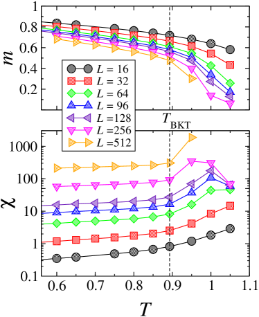
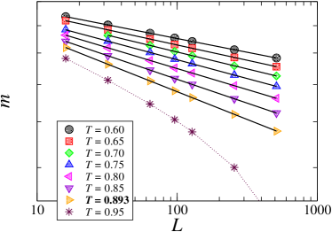
We can observe in figure (1) a progressive decrease of the magnetization with the system size, at constant temperatures. Moreover, as become evident from figure (2), we see that these decays follow power-laws with the system size in the whole range $T\leq T_{BKT}$, according to the FSS picture in the critical phase, $m\sim L^{-\frac{1}{2}\eta(T)}$, with an exponent $\eta(T)$ which depends on the value of the temperature (to be discussed in the next section). When the value of the temperature is above $T_{BKT}$, the decay of the magnetization is faster than a power law.

Figure 2: Behaviour of the magnetization versus the system size at different temperatures for the 2D XY-model. Power-law behaviours appear in the whole range $T\leq T_{BKT}$. (Monte Carlo simulations with $10^{6}$ MCS/spin after removing the first $10^{6}$ MCS to achieve proper thermalization).

Figure 3: Behaviour of the magnetic susceptibility versus the system size at various temperatures for the 2D XY-model. (Monte Carlo simulations with $10^{6}$ MCS/spin after removing the first $10^{6}$ MCS to achieve proper thermalization).

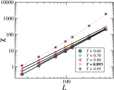
On the other hand, the magnetic susceptibility at fixed temperature (figure 1) exhibits regular increase with the system size for all temperatures at and below $T_{BKT}$. It is in contrast with an ordinary second order phase transition in which the susceptibility diverges only at the critical temperature. In particular, the susceptibility exhibits power law behaviours with $L$ for any $T\leq T_{BKT}$ (figure 3). It is interesting to notice that a change in the exponent of the power-law of the susceptibility with the system size, appears at $T_{BKT}$.

Also, we see in figure (1), that the susceptibility reaches its maximum value systematically above $T_{BKT}$. The temperature at which this maximum occurs tends to $T_{BKT}$ when $L\rightarrow\infty$.

The power law behaviours of the magnetization and of the magnetic susceptibility at low temperatures, can be interpreted as evidences of a QLRO phase for the 2D XY-model in the thermodynamic limit, in the temperature range $T<T_{BKT}$.

III.2 The 2D Heisenberg model

The 2D Heisenberg model is expected not to exhibit any phase transition polya ; brez ; amitbook ; izyu . The magnetic susceptibility strongly diverges when the temperature vanishes polya . However, some authors argued in favour of a transition Niedemayer ; PatrasciouSeiler ; Patrasciou ; Aguado and possibly an effective quasi-long-range-ordered phase tesisAna ; bb at very low temperatures, at least in large but finite systems.

Figure 4: Temperature dependence of thermodynamic quantities for the 2D Heisenberg model. Top: magnetization (m). Bottom: susceptibility ($\chi$). (Monte Carlo simulations with $10^{6}$ MCS/spin after removing the first $10^{6}$ MCS to achieve proper thermalization).

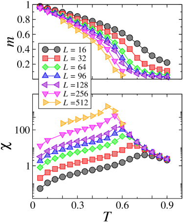
In figure (4), one can see the behaviours of the magnetization and of the magnetic susceptibility with the system size and temperatures for the 2D Heisenberg model. We can notice the decrease of the values of the inflection point of $m$ versus $T$, when the system size increases. On the same way, the temperatures where the susceptibility reaches the maximum, are displaced to lower and lower values when the system sizes are larger. As a matter of fact, if there is a positive critical temperature analogous to the $T_{BKT}$, its value should be quite small, at the thermodynamic limit.

III.3 The 2D LL-model

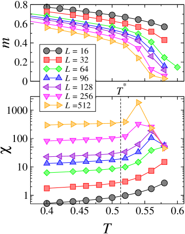
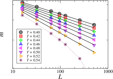
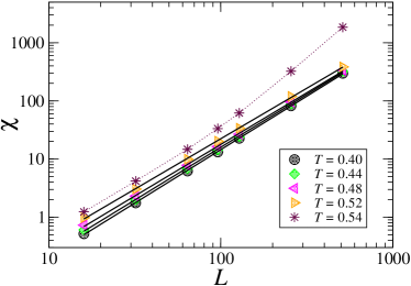
We analyze now the magnetization and the magnetic susceptibility of the 2D Lebwohl-Lasher model, using the same procedure as for the 2D XY-model. In figure (5) the magnetization, $m$, and the magnetic susceptibility, $\chi$, are shown versus the temperature for various lattice sizes $L$. There is a complete qualitative agreement with the behaviour of the same quantities for the 2D XY-model (figure 1). Indeed the “critical” temperature is shifted to $T^{\star}=0.513$ kuzu ; FPB , but all the power-law behaviours are equally recovered (figures 6 and 7), and even the change, at $T^{\star}$, of the apparent value of the exponent of the susceptibility versus the system size, or the asymptotic convergence to $T^{\star}$, of the temperatures at which the susceptibility reaches its maximum are identically noticed.

Figure 5: Temperature behaviour of thermodynamics quantities for the 2D Lebwohl-Lasher model. Top: magnetization (m). Bottom: magnetic susceptibility ($\chi$). (Monte Carlo simulation with $10^{6}$ equilibrium steps (measured as the number of flipped Wolff clusters) after removing the first $10^{6}$ MCS to achieve proper thermalization).

Figure 6: Behaviour of the magnetization with the system size at various temperatures for the 2D LL-model. (Monte Carlo simulation with $10^{6}$ equilibrium steps (measured as the number of flipped Wolff clusters) after removing the first $10^{6}$ MCS to achieve proper thermalization).

Figure 7: Behaviour of the magnetic susceptibility versus the system size at various temperatures for the 2D LL-model. (Monte Carlo simulation with $10^{6}$ equilibrium steps (measured as the number of flipped Wolff clusters) after removing the first $10^{6}$ MCS to achieve proper thermalization).

III.4 Conclusion from the study of the $m$ and $\chi$ behaviours

From this preliminary analysis, one could conclude that the 2D LL-model behaves similarly to the 2D XY-model. Namely, one can define a BKT temperature, $T^{\star}$, at which the system is critical, and a QLRO phase seem to occur at temperatures smaller than $T^{\star}$.

We shall see below that this anticipated conclusion is refuted by more refined analysis.

IV Calculations of the correlation function exponent $\eta$

In principle, very precise information can be obtained from the estimates of the fundamental critical exponent $\eta$ for the pair correlation function. This exponent may depend on the effective temperature $T$ in the case of a continuous line of critical points.

Several methods can be used independently in the case of the BKT transition. We shall use the following ones below:

• Finite size scaling behaviour of the magnetization.

  At the critical point of a second order phase transition, the magnetization $m$ behaves as a power law of the system size, namely: $m\sim L^{-\beta/\nu}$. This combination of critical exponents is related to the exponent which describes the critical decay of appropriate pair correlation function, $G(r)\sim r^{-(d-2+\eta)}$, $2\beta/\nu=d-2+\eta$, thus in two dimensions $m\sim L^{-\frac{1}{2}\eta}$. Here, $\eta$ is a function of $T$ and FSS is used to estimate the critical exponents at different temperatures (in the low temperature phase) from figure (2) or figure (6) ;

• FSS behaviour of the magnetic susceptibility.

  The magnetic susceptibility, $\chi$, scales as a power law involving the critical exponents $\gamma$ and $\nu$, namely: $\chi\sim L^{\gamma/\nu}$. Then, the hyperscaling relation

  $$\eta=2-\gamma/\nu,$$ (3)

  holds, which gives an alternative estimate of the exponent $\eta$. Here too, FSS may be used to extract an appropriate exponent from the data of figure (3) or figure (7);

• Conformal Transformation (CT) method.

  Another tool can be used to estimate the value of $\eta$ for very large systems: the conformal transformation method (see Cardy Cardy ). It is indeed a powerful method which applies to analyze any conformally covariant density profile (or correlation function) from the mapping of infinite or semi-infinite geometries onto restricted geometries where simulations are actually performed berche03 ; ResStraley00 . We thus consider a density profile $m(w)$ in a finite system with symmetry breaking fields along some edges in order to induce a non-vanishing local order parameter in the 2D bulk of the system. Here, $w$ stands for the location in the finite system. In the case of a square lattice of size $L\times L$, with fixed boundary conditions along the four edges, using a simple mathematical transformation – called the Schwarz-Christoffel transformation derridaburkhardt ; chatelain – one expects a power law in terms of an effective locally rescaled distance

  $$m(w) \sim [\kappa(w)]^{-\frac{1}{2}\eta}.$$ (4)

  This method has been used extensively in berche03 ; EPL to estimate the pair correlation exponent as a function of temperature for the 2D XY-model;

• Systems in an applied magnetic field.

  According to the scaling hypothesis, the magnetization of a general $d$-dimensional system at a critical temperature, must follow the scaling law:

  $$m=H^{1/\delta}G(L^{-1}H^{-1/y_{h}}),$$ (5)

  where $H$ is the applied magnetic field. The magnetic exponent is given in terms of the magnetic field scaling dimension $y_{h}$, $\delta=y_{h}/(d-y_{h})$, and $G$ is a universal function golden . In the thermodynamic limit $L^{-1}H^{-1/y_{h}}\ll 1$, the system follows the singular behaviour $m\sim H^{1/\delta}$. In the other limit $L^{-1}H^{-1/y_{h}}\gg 1$, the magnetization follows $m\sim L^{y_{h}-d}$. As we know that $m\sim L^{-\eta/2}$ for the BKT transition, one deduces in this case the hyperscaling relation under the form:

  $$d-y_{h}=\eta/2.$$ (6)

  which again can be used to estimate the value of $\eta$.

IV.1 The 2D XY-model

The FSS methods are used from figure (2) and figure (3). The results obtained by the CT method are from the reference EPL .

Figure 8: XY-model in a magnetic field H. For each temperature the system sizes are: $L=32$, $64$, $96$, $128$, and the magnetic field strengths are: $H=0.1$, $0.01$, $0.05$, $0.001$, $0.005$, $0.0001$, $0.0005$. The bold straight lines represent the large $X=HL^{y_{h}}$ limit for a Weibull-like PDF (W) for each temperature. The number of Wolff steps for each $T$, $L$ and $H$ is $2\times 10^{5}$.

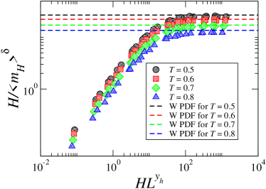
We add here a few words about the 2D XY-model in a magnetic field. The exponent $\eta$ at the BKT transition is $1/4$, then $y_{h}=15/8$, and $\delta=15$ has the same value as for the $d=2$ Ising model. Using equation (5), an excellent collapse of $Y=H/m^{\delta}$ versus $X=HL^{y_{h}}$ at $T_{BKT}=0.893$ has been obtained in rprb . The authors obtained in this work the additional result that $Y$ tends to a constant value in the limit $HL^{y_{h}}\rightarrow\infty$. The saturation of $Y$ for large magnetic fields means a Weibull-like fieldless probability distribution function (PDF) bouk for the magnetization. We extended in the present work this result to other temperatures.

Figure 9: Dependence of the correlation function critical exponent with the temperature for the 2D XY-model. (Monte Carlo simulations with $10^{6}$ MCS/spin after removing the first $10^{6}$ MCS to achieve proper thermalization). The conformal transformation (CT) values are from the reference EPL . The dashed line is the spin-wave result $\eta=k_{B}T/2\pi J$.

Indeed, for a BKT transition there is a line of critical points for any $T\leq T_{BKT}$, and the equation (5) must be satisfied in all this range of temperatures. Then, we performed numerical simulations of the 2D XY-model in an applied magnetic field wolffH for temperatures below $T_{BKT}$. Figure (8) shows the excellent collapse of the data, as well as the saturation of $Y$ for several magnetic field strengths and several system sizes, at all the temperatures $\leq T_{BKT}$ investigated. The collapse of the data gives an estimate of the critical exponent $\eta(T)$ using the hyperscaling relation (6).

This result invalidates a claim by Bramwell et al. bram1 , about the possible Gumbel-like distributions bouk of the magnetization in the 2D XY-model at low temperatures. Indeed, the Gumbel PDF does not lead to the saturation of the function $Y$ in the limit $HL^{y_{h}}\rightarrow\infty$.

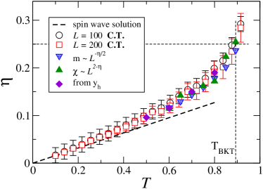
The figure (9) shows the values of the critical exponent $\eta$ for the 2D XY-model, calculated from FSS using the magnetization or the magnetic susceptibility, with the CT method (from EPL ), and using the collapse of the data for the system in a magnetic field. All the methods lead to determinations of $\eta$ which are in excellent agreement with each other.

However, one can note that the behaviour obtained with CT is the most precise, because this method is able to reach the behaviour of the infinite-size systems, with system sizes computationally accessible, all shape effects being encoded (in the continuum limit) in the conformal mapping (hence the name of Finite Shape Scaling that we tried to introduce in Ref. FPB2 ). The differences between the results obtained from $m$ and from $\chi$, are of the order of $5\%$. In the references RAR and rprb , the authors used more than $6\times 10^{6}$ independent realizations for the estimate of the exponent $\eta$. Realization of the hyperscaling relation (3) has been checked with a relative error smaller than $0.4\%$.

More than simple illustrations, these results allow us to compare the effeciency of the different methods for the proper definition of a quasi-long-range-order phase in systems with continuous symmetry.

IV.2 The 2D Heisenberg model

We compare now the values measured for $\eta$ for a system (the 2D Heisenberg model) which does not exhibit any transition, at least for temperatures above $T=0.1$ polya (see figure 4)). Then, we can expect the behaviours of $\eta$ to be quite different in the two cases.

Figure 10: Dependence of the effective correlation function critical exponent with the temperature for the 2D Heisenberg model. The dashed line is the spin-wave result $\eta=k_{B}T/\pi J$ bb .

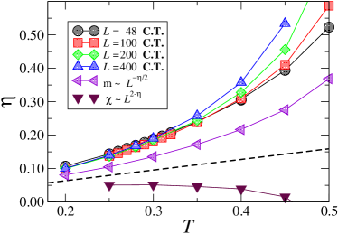
The figure (10) shows the values of $\eta$ calculated using the FSS and the CT methods for the 2D Heisenberg model. The differences with the 2D XY-model are clear. It is particularly noticeable that the estimates given by the three methods are completely different. Even the shapes of the curves are different, and no agreement can be found. In particular, the determinations of $\eta$ deduced from $m$ and $\chi$, respectively, do not agree with each other. It follows that the hyperscaling relation (3) is definitively not satisfied.

These observations give a strong evidence for the lack of any critical behaviour in the 2D Heisenberg model within the range of temperatures considered here.

IV.3 The 2D LL-model

We present now a similar systematic work, performed on the 2D LL-model. In particular, the figure (11) shows results for the 2D LL-model in an applied magnetic field at the expected critical temperature, $T^{\star}$.

Figure 11: 2D Lebwohl-Lasher model in a magnetic field ($H=0.1$, $0.01$, $0.05$, $0.001$, $0.005$, $0.0001$, $0.0005$) at $T=0.513$. The bold straight line represents the large $X=HL^{y_{h}}$ limit for a Weibull-like PDF (W). Each point corresponds to an average over $100,000$ independent realizations.

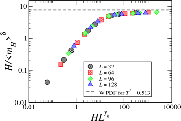
The results are consistent with the equation (5), and with the saturation of the quantity $Y$. The best collapse was obtained for $\delta=10.83$. Then, using the hyperscaling relation (6) we found: $\eta=0.338$ at this temperature. This result is shown in figure (12) and the agreement with the value of $\eta$ obtained from the other methods is excellent at this temperature.

Figure 12: Dependence of the critical exponent $\eta$ with the temperature for the 2D Lebwohl-Lasher model. (Monte Carlo simulations with $10^{6}$ MCS/spin after removing the first $10^{6}$ MCS to achieve proper thermalization). The conformal transformation (CT) data are from reference FPB . The dashed line is the spin-wave result $\eta=4k_{B}T/3\pi J$.

In figure (12), we show the values of $\eta$ for the 2D LL-model at various temperatures. Estimates were done using FSS of the magnetization (from reference PFB and figure 6) and of the magnetic susceptibility (from figure 7). They are compared to the values estimated from the CT method (from reference FPB ), and from the collapse of the data in a magnetic field.

Nevertheless, one should stress that the agreement between the values estimated by all the four methods is good, but imperfect. Small discrepancies can easily be noticed. In particular, the estimates which are based on the FSS behaviour of the magnetic susceptibility are systematically smaller than those following from the other methods. The errors are larger than $10\%$, a relevant quantity probably far out of the range of acceptable error bars. In a previous work RAR , this error was only of $3\%$, but the authors then checked systematically the hyperscaling relation, equation (3), and they concluded that the hyperscaling relation is definitively not satisfied at low temperature (e.g. at $T=0.4)$ (see discussion in the section V below). This has been the first evidence for absence of a QLRO phase in the 2D LL-model.

V Revisiting the behaviour of the 2D LL-model at the ‘critical’ temperature

In the previous section, we observed that the critical behaviour of the 2D XY-model and the behaviour of the 2D LL-model were quite similar. Nevertheless, we saw small discrepancies for the LL-model, in particular in the behaviour of the second moment of the magnetization, and on the validity of the hyperscaling relation (3).

In reference RAR , the authors performed intensive simulations of the 2D LL-model at the temperature $T=0.4$ well below the expected critical temperature. Clear failure of the hyperscaling relation, failure of collapse of the PDF in the first scaling form bp , and analysis of the Binder cumulant, led to the conclusion that no QLRO phase exists in the 2D LL-model at this temperature.

Here, we consider the problem of the existence of a critical at the temperature $T^{\star}=0.513$, as this temperature was reported as a possible BKT temperature for the 2D LL-model (see section III and references kuzu ; FPB ). To elaborate on this question, we will report results about the probability distribution function, the magnetization scaling and the hyperscaling relation (3) at this temperature. We shall also compare the stiffness for the LL- and XY-models.

V.1 The first-scaling law

Figure 13: PDF of the magnetization for the 2D Lebwohl-Lasher model at the temperature $T^{\star}=0.513$, plotted in the first-scaling form (7). The scaling law is not confirmed for $L=32$ up to $L=256$. Wolff’s single-cluster algorithm was used wolff . Each data set corresponds to average over $6,000,000$ independent realizations.

If the 2D Lebwohl-Lasher model is critical at the temperature $T^{\star}=0.513$, self-similarity must be observed at this temperature because no finite characteristic length can exist at criticality. Asymptotic self-similarity results in the so-called first-scaling law for the order parameter, here the magnetization $m$, bp :

$$\langle m\rangle P(m)\equiv\Phi_{T}(z_{1}),\;\;\;\;\;\;\mbox{with}\;\;z_{1}\equiv\frac{m}{\langle m\rangle},$$ (7)

with $\Phi_{T}$ a scaling function which depends only on the actual temperature $T$. Equation (7) is sequel of the standard finite-size scaling theory cardy , but it is highly advantageous that equation (7) does not require knowledge of the values of any critical exponent. Note that, under this form, the hyperscaling relation,

$$\frac{\langle m\rangle}{\sigma}\quad=\quad\mbox{ constant term},$$ (8)

is automatically realized with $\sigma$ the standard deviation of the order parameter. Indeed, one has: $\sigma^{2}\propto\chi/L^{d}$, and $\sigma$ scales then with the system size as: $\sigma\sim L^{\gamma/2\nu-1}$ for 2D systems. Therefore, the ratio $\langle m\rangle/\sigma$ should be a constant whenever the hyperscaling relation (3) is satisfied RAR .

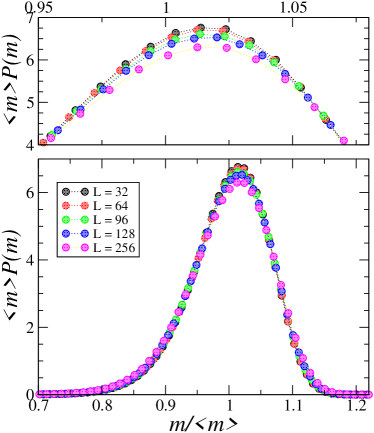
Figure (13) shows the behaviour of the PDF when the system size increases, for the 2D LL-model at the temperature $T^{\star}=0.513$. We can observe failure of the collapse between these curves, specially for the largest system sizes, where the distributions tend to deviate from each other when $L$ increases. One must conclude that the temperature $T^{\star}=0.513$ is not critical for this model.

In two others papers published recently, one can find the same kind of curve for the 2D XY-model at $T=0.6<T_{BKT}$ RAR and at $T=T_{BKT}$ rprb . The collapse of all the PDF is excellent in the two cases, a result consistent with the known criticality of the system at $T_{BKT}$ and all the temperatures below this value. In the same reference RAR , the 2D LL-model was studied similarly at $T=0.4$. Failure of the collapse was clear in this case, leading to the conclusion that the system is not critical below the assumed transition temperature.

Figure 14: PDF of the magnetization for the Lebwohl-Lasher model at $T=0.548$, plotted in the first-scaling form (7). Each data set corresponds to average over $6,000,000$ independent realizations.

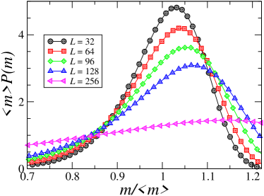
In 2003, Mondal et al. mr reported a possible transition temperature for the 2D LL-model at the temperature $T=0.548$, larger than the values reported by Kunz et al in 1992 kuzu . We thus also performed numerical simulations of the 2D LL-model at $T=0.548$. In figure (14) the data are plotted in the first-scaling form (7). The data are far from collapsing. It is actually similar to the behaviour of a system far away from any critical point.

Figure 15: $m/\sigma$ vs. $L^{-1}$ at $T=T_{BKT}$ for the 2D XY-model (top) and at $T=T^{\star}=0.513$ for the 2D Lebwohl-Lasher model (bottom). For the XY-model, the data were obtained from the reference rprb . For the LL-model, the blue line is a power law fit.

V.2 The hyperscaling relation

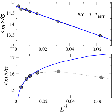
In this section, we check numerically the hyperscaling relation under the form (8). In figure (15), $\langle m\rangle/\sigma$ is plotted versus $1/L$ for the 2D XY-model and the 2D LL-model respectively, at the BKT temperatures reported or expected for each system, namely: $T_{BKT}=0.893$ for the XY-model and $T^{\star}=0.513$ for the LL-model.

For the XY-model, the ratio is seen to converge to a definite value ($\simeq 14.8$) at the thermodynamic limit $1/L=0$, while for the LL-model, a power law is the best fit consistent with the data of $\langle m\rangle/\sigma$ versus $L$, and this fit leads to a vanishing value of the ratio at the thermodynamic limit. We conclude that the hyperscaling relation is very likely violated in this case, for the obvious reason that the system is not critical at the temperature $T^{\star}=0.513$.

V.3 The stiffness modulus

Appearance of stiffness is an important consequence of the spontaneous symmetry breakdown in a system with continuous symmetry. It is closely related to correlations in the transverse response function, any spatial variation of the order parameter, perpendicular to the direction of the ordering, increasing the energy of the system. For this reason, the system generates a restored strength in response to any attempt to create a new configuration: this is known as stiffness.

In the case of the 2D XY-model, this is the helicity modulus and it is defined as follows. Let

$${\cal H}=-\beta J\sum_{\langle i,j\rangle}{\bf S}_{i}\cdot\hat{g}_{\alpha}{\bf S}_{j}$$ (9)

be the modified Hamiltonian in which $\hat{g}_{\alpha}$ is a rotation of angle $\phi$ of the system around any axis, say here the $x$-axis. The difference between the free energy $F(\phi)$ calculated with the modified Hamiltonian, and the free energy calculated with the original Hamiltonian,

$$F(\phi)-F(0)=-\frac{1}{\beta}\ln\left(\frac{{\rm Tr\ \!}{\rm e}^{-\beta{\cal H}_{g_{x}}}}{{\rm Tr\ \!}{\rm e}^{-\beta{\cal H}_{0}}}\right),$$ (10)

varies quadratically with the rotation angle $\phi$, at least for $\phi\ll 1$. The coefficient, usually written: $\Upsilon$, is the helicity modulus:

$$F(\phi)-F(0)=-\Upsilon\phi^{2}+O(\phi^{4})$$ (11)

and it takes the form

$$\frac{2L^{d}}{J\beta}\Upsilon=\left\langle\sum_{\langle i,j\rangle}{\bf S}_{i}\cdot\hat{J}_{x}^{2}{\bf S}_{j}\right\rangle-J\left\langle\Bigl{(}\sum_{\langle i,j\rangle}{\bf S}_{i}\cdot\hat{J}_{x}{\bf S}_{j}\Bigr{)}^{2}\right\rangle$$ (12)

where $\hat{J}_{x}$ is the rotation operator around the $x$-axis.

Figure 16: Temperature behaviour of the stiffness modulus $\Upsilon$ for the 2D XY-model. (Monte Carlo simulations with $10^{6}$ MCS/spin after removing the first $10^{6}$ MCS to achieve proper thermalization).

Figure 17: Temperature behaviour of the stiffness modulus $\Upsilon$ for the 2D Lebwohl-Lasher model. (Monte Carlo simulations with $10^{6}$ MCS/spin after removing the first $10^{6}$ MCS to achieve proper thermalization).

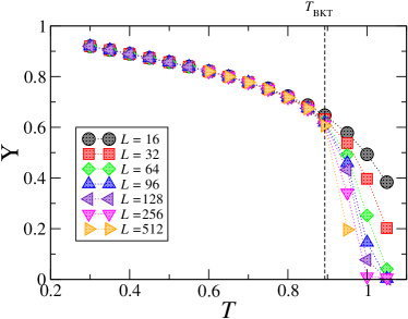
In figure (16) the stiffness modulus for the 2D XY-model is shown versus the temperature for various sizes from $L=16$ to $L=512$. The behaviour is typical of an order parameter: below $T_{BKT}=0.893$, the plots are almost independent of the system size, and this is the sign of the rigid phase with a finite value of the stiffness constant, while for temperatures larger than $T_{BKT}=0.893$, the system’s response becomes weaker, leading to the decrease of the stiffness modulus. The high-temperature phase is a disordered phase with the vanishing stiffness. The change of behaviour in the stiffness modulus between the two phases exhibits the appearance of a topological phase transition, with quasi-long-range order, but finite rigidity, in the low temperature phase.

For the 2D LL-model, the same procedure can be used with eventually the following expression for the stiffness:

$$\frac{2L^{d}}{3J\beta}\Upsilon=-\left\langle\sum_{<i,j>}\left(({\bf S}_{i}\cdot{\bf S}_{j})\times({\bf S}_{i}\cdot\hat{J}_{x}^{2}{\bf S}_{j})+({\bf S}_{i}\cdot\hat{J}_{x}{\bf S}_{j})^{2}\right)\right\rangle+3J\left\langle\Bigl{(}\sum_{<i,j>}({\bf S}_{i}\cdot{\bf S}_{j})\times({\bf S}_{i}\cdot\hat{J}_{x}{\bf S}_{j})\Bigr{)}^{2}\right\rangle$$ (13)

Figure 18: Stiffness $\Upsilon$ versus system size $L$ for three different temperatures for the 2D XY-model. $\Upsilon(L)$ goes to a finite value in the limit $L\rightarrow\infty$ for $T\leq T_{BKT}$. (Monte Carlo simulations with $10^{6}$ MCS/spin after cancellation of $10^{6}$ for thermalization).

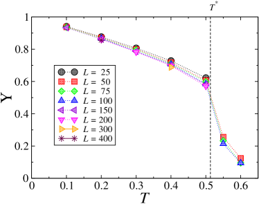
Then, we have plotted $\Upsilon$ versus the temperature as it is shown in figure (17) for various sizes from $L=25$ to $L=400$. Again, a behaviour similar to an order-parameter is observed in this case. At any temperature below $T^{\star}=0.513$, one clearly identifies finite values of the stiffness independently of the system size. Above $T^{\star}$, the values of the stiffness drop to values close to $0$.

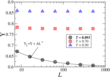
However, beyond the similarities, one can remark that the stabilization to a finite value of the stiffness in the low-temperature phase, is not similar in both models. One can see this point, in particular analyzing the dependences with the system size. In figure (18), $\Upsilon$ is shown versus $L$ for three different temperatures of the 2D XY-model. Two of them below the BKT transition ($T=0.5$ and $0.7$), and the other temperature just at the BKT transition. For the lower temperatures $\Upsilon$ goes fast to an asymptotic constant value. At $T_{{BKT}}$, the stiffness modulus reaches its saturation value algebraically. Then, it is clear that for the XY-model a sharp jump of the stiffness modulus is observed right at the topological transition.

Figure 19: Behaviour of stiffness modulus versus the system size for the 2D Lebwohl-Lasher model. (Monte Carlo simulations with $10^{6}$ MCS/spin after removing the first $10^{6}$ MCS to achieve proper thermalization).

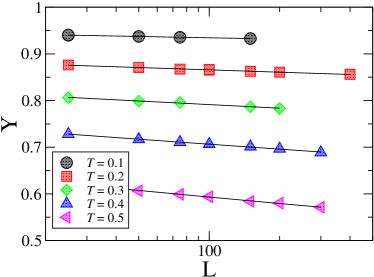
The behaviour is completely different for the 2D LL-model. In figure (19), the dependence of $\Upsilon$ with the system size $L$ is shown for various temperatures below $T^{\star}$. The stiffness does not reach a finite value in the limit $L\rightarrow\infty$. This behaviour is similar to the 2D Heisenberg model MouhannaEPL and to the fully frustrated Heisenberg model Wintel . In figure (19), the slopes of the curves depend on the value of the temperature. It appears to be similar to the results of Winttel et al Wintel . A detailed study of the stiffness for frustrated spin systems can be found in MouhannaPRB .

VI Discussion and Conclusions

Our initial goal was to give definite conclusions about the possible appearance of a critical topological transition, for example of the Berezinskii-Kosterlitz-Thouless type, in the 2D Lebwhol-Lasher model.

Our results exhibit a scenario more complex than expected. It can be summarized as follows:

• The behaviour of the order parameter (the magnetization) with the temperature and the system size, pointed out a quasi-long range order phase for temperatures below the value $T^{\star}=0.513$. One has noticed an excellent agreement of the correlation exponent $\eta$ estimated using conformal transformation, scaling of the order parameter with $L$, including scaling with a magnetic field.

• If we investigate a quantity related to the second moment of the order parameter, that is the susceptibility, a qualitative agreement with a QLRO phase behaviour is observed. However, the value obtained for $\eta$ from this quantity does not compare well with the estimates from the order parameter. Actually, the hyperscaling relation (3) is not satisfied for $T\leq T^{\star}$. This is in clear contradiction with the possibility of a line of critical point below $T^{\star}$. Then, one has to conclude that a BKT transition is not observed for this model.

• Although not studied in the present paper, the behaviour of the Binder cumulant (which depends on the fourth moment of the order parameter), as reported in RAR , fully supports the above conclusion: no universality is observed at any finite temperature. Signs of QLRO just disappear if larger moments of the order parameters are used.

• As the conclusion seems to depend on the order of the moment of the magnetization, it looks natural to use the complete probability distribution function of the order parameter to clarify the situation. Unlike the 2D XY-model, the 2D LL-model does not show any first-scaling-law collapse as it would be expected for a critical system. The absence of self-similarity at any temperature discards any sort of transition in this model, which thus appears more similar to the Heisenberg model than to the XY-model eventually.

• The stiffness modulus mixes a second and a fourth moment of the order parameter. For the 2D LL-model, this quantity does not exhibit an order-parameter behaviour. At low temperatures a logarithmic decay with $L$ is observed, and asymptotic finite values are highly unlikely, resulting in a non rigid phase at low temperatures.

Our conclusion, based only on numerical simulations, is that the 2D LL-model shares similarities with the fully frustrated antiferromagnetic Heisenberg model (see Wintel ; Kawamura ). Then, the overall behaviour could well be a sharp crossover Wintel , instead of a real transition to a critical phase, a new kind of frustration preventing the topological defects of the LL-model to initiate a true phase transition.

References

- (1) Zewdie H., Bull. Chem. Soc. Ethiop., 2000, 14, 69.
- (2) Zhang Z., Mouritsen O.G., Zuckermann M., Phys. Rev. Lett., 1992, 69, 2803.
- (3) Mermin N. D., Wagner H., Phys. Rev. Lett., 1966, 22, 1133.
- (4) Hohenberg P.C., Phys. Rev., 1967, 158, 383.
- (5) Mermin N.D., J. Math. Phys., 1967, 8, 1061.
- (6) Mermin N.D., Phys. Rev., 1968, 176, 250; erratum Phys. Rev. B, 1979, 20, 4762.
- (7) Coleman S., Commun. Math. Phys., 1973, 31, 259.
- (8) Berezinskii V.I., Sov. Phys. JETP, 1971, 34, 610.
- (9) Kosterlitz J.M., Thouless D.J., J. Phys. C, 1973, 6, 1181.
- (10) Polyakov A.M., Phys. Rev. B, 1975, 59, 79.
- (11) Brézin E., Zinn-Justin J., Phys. Rev. B, 1976, 14, 3110.
- (12) Amit D. J., Field Theory, The Renormalization Group and Critical Phenomena. World Scientific, Singapore, 1984.
- (13) Izyumov Yu.A., Skryabin Yu.N., Statistical Mechanics of Magnetically Ordered Systems. Kluwer Academic Publishers, New York, 1988.
- (14) Niedermayer F., Niedermaier M., Weisz P., Phys. Rev. D, 1997, 56, 2555.
- (15) Patrascioiu A., Seiler E., Phys. Rev. Lett., 1995, 74, 1920; J. Stat. Phys., 2002, 106, 811; Phys. Rev. B, 1996, 54, 7177; Phys. Rev. D, 1998, 57,1394.
- (16) Patrascioiu A., Europhys. Lett., 2001, 54, 709.
- (17) Aguado M., Seiler E., Phys. Rev. D, 2004, 70, 107706.
- (18) Fariñas-Sánchez A.I., Ph.D. thesis. Instituto Venezolano de Investigaciones Científicas, Caracas, Venezuela, 2004; Ph.D. thesis. Université Henri Poincaré-Nancy 1, France, 2004.
- (19) Kapikranian O., Berche B., Holovatch Yu., J. Phys. A: Math. Theor., 2007, 40, 3741.
- (20) Lebwohl P.A., Lasher G., Phys. Rev. A, 1973, 6, 426.
- (21) Maier W., Saupe A., Z. Naturforsch., 1959, 14A, 882.
- (22) Kunz H., Zumbach G., Phys. Rev. B, 1992, 46, 662.
- (23) Blote H.W.J., Guo W., Hilhorst H.J., Phys. Rev. Lett., 2002, 88, 047203.
- (24) Caracciolo S., Pelissetto A., Phys. Rev. E, 2002, 66, 016120.
- (25) Fariñas-Sánchez A.I., Paredes R., Berche B., Phys. Lett. A, 2003, 308, 461.
- (26) Paredes R., Fariñas-Sánchez A.I., Berche B., Rev. Mex. Fis., 2006, 52, 181.
- (27) Fariñas-Sánchez A.I. , Paredes R., Berche B., Phys. Rev. E, 2005, 72, 031711.
- (28) Berche B., Paredes R., Cond. Matt. Phys., 2005, 8, 723.
- (29) Binder K., Z. Phys. B, 1981, 43, 119.
- (30) Mondal E., Roy S. K., Phys. Lett. A, 2003, 312, 397.
- (31) Dutta S., Roy S.K., Phys. Rev. E, 2004, 70, 066125.
- (32) Paredes R., Fariñas-Sánchez A.I., Botet R., Phys. Rev. E., 2008, 78, 051706.
- (33) Botet R., Płoszajczak M., Latora V., Phys. Rev. Lett., 1997, 78, 4593.
- (34) Wolff U., Phys. Rev. Lett., 1989, 62, 361.
- (35) Cardy J.L., in Phase Transitions and Critical Phenomena, vol. 11. Edited by C. Domb and J.L. Lebowitz, Academic, London, 1987.
- (36) Berche B., J. Phys. A, 2003, 36, 585.
- (37) Reš I., Straley J., Phys. Rev. B, 2000, 61, 14425.
- (38) Burkhardt T.W., Derrida B., Phys. Rev. B, 1985, 32, 7273.
- (39) Chatelain C., Berche B., Phys. Rev. E, 1998, 58, R6899.
- (40) Berche B., Fariñas-Sánchez A.I., Paredes R., Europhys. Lett., 2002, 60, 539.
- (41) Goldenfeld N., Lectures on Phase Transitions and the Renormalization Group. Addison-Wesley Publishing Company, 1992.
- (42) Paredes V. R., Botet R., Phys. Rev. E., 2006, 74, 060102(R).
- (43) Botet R., Płoszajczak M., Universal Fluctuations. World Scientific Lecture Notes in Physics, vol. 65. World Scientific, Singapore, 2002.
- (44) For the 2D XY-model or 2D LL-model in the magnetic field , we used a Wolff algorithm similar to the one used for the case, with an additional spin which interacts with all the other spins, with as the strength of the interaction.
- (45) Bramwell S.T. et al., Phys. Rev. Lett., 2000, 84, 3744.
- (46) Finite-Size Scaling. Edited by J. Cardy, North-Holland, Amsterdam, 1988.
- (47) Caffarel M., Azaria P., Delamotte B., Mouhanna D., Europhys. Lett., 1994, 26, 493.
- (48) Wintel M., Everts H.U., Apel W., Phys. Rev. B, 1995, 52 13480.
- (49) Caffarel M., Azaria P., Delamotte B., Mouhanna D., Phys. Rev. B, 2001, 64, 014412.
- (50) Kawamura H., Kikuchi M., Phys. Rev. B, 1993, 47, 1134.