Characterization of the BICEP Telescope for High-Precision
Cosmic Microwave Background Polarimetry
Abstract
The Bicep experiment was designed specifically to search for the signature of inflationary gravitational waves in the polarization of the cosmic microwave background (CMB). Using a novel small-aperture refractor and 49 pairs of polarization-sensitive bolometers, Bicep has completed 3 years of successful observations at the South Pole beginning in 2006 February. To constrain the amplitude of the inflationary -mode polarization, which is expected to be at least 7 orders of magnitude fainter than the 3 K CMB intensity, precise control of systematic effects is essential. This paper describes the characterization of potential systematic errors for the Bicep experiment, supplementing a companion paper on the initial cosmological results. Using the analysis pipelines for the experiment, we have simulated the impact of systematic errors on the -mode polarization measurement. Guided by these simulations, we have established benchmarks for the characterization of critical instrumental properties including bolometer relative gains, beam mismatch, polarization orientation, telescope pointing, sidelobes, thermal stability, and timestream noise model. A comparison of the benchmarks with the measured values shows that we have characterized the instrument adequately to ensure that systematic errors do not limit Bicep’s 2-year results, and identifies which future refinements are likely necessary to probe inflationary -mode polarization down to levels below a tensor-to-scalar ratio .
Subject headings:
cosmic background radiation — cosmology: observations — gravitational waves — inflation — instrumentation: polarimeters — telescopes1. Introduction
A strong indication of an inflationary origin of the universe would be a detection of the curl component (“-mode”) in the polarization of the CMB arising from gravitational wave perturbations (Dodelson et al., 2009). This primordial -mode polarization is expected to peak at angular scales of 2∘, and the magnitude of the power spectrum is described by the ratio of the initial tensor-to-scalar perturbation amplitudes, a quantity directly related to the energy scale of inflation. The best published upper limit is at 95% confidence, derived from CMB temperature anisotropy measurements at large angular scales combined with constraints from Type Ia supernovae and baryon acoustic oscillations (Komatsu et al., 2009). Upper limits on the -mode polarization amplitude, , of 0.8 K rms have been placed by at a multipole moment of 65 and by QUaD at 200, respectively (Nolta et al., 2009; Pryke et al., 2009). These limits are still well above the expected levels of confusion from either polarized Galactic foregrounds in the cleanest regions of the sky or from gravitational lensing that converts the much brighter CMB gradient (“-mode”) polarization to -modes at smaller angular scales.
Bicep (Background Imaging of Cosmic Extragalactic Polarization) is an instrument designed to target the expected peak of the gravitational-wave signature at angular scales around 2∘. Using proven bolometric technologies and selecting the cleanest available field for observation, this instrument was designed, given sufficient observation time, to be capable of measuring a polarization signal of 0.08 K rms at 100 corresponding to the BB signal expected for a tensor-to-scalar ratio of . The CMB temperature anisotropy has a much larger amplitude of 50 K rms at these angular scales, and imperfect rejection of it in the polarization measurement could result in a residual false signal. In addition, errors in polarization orientations and pointing could mix the 1 K -mode CMB polarization signal into spurious -modes. This experiment therefore requires careful instrument characterization and calibration to minimize systematic contamination in the polarization measurement.
This paper supplements a companion paper that presents the CMB polarization power spectra from the first 2 years of Bicep data (Chiang et al., 2010). The rest of this section gives an overview of the instrument, the observing strategy, and the collected data. Section 2 describes the simulations that determine the impact of the instrumental parameter characterization on the cosmological results. Section 3 describes each of the instrumental properties and how we calibrate them. Section 4 discusses how we characterize the properties of noise in our data and quantify the noise bias through simulations. We conclude by identifying what we find to be the most important systematic uncertainties for Bicep and discussing the path forward toward improving these uncertainties for future, more sensitive, measurements.
1.1. Instrument design overview
|
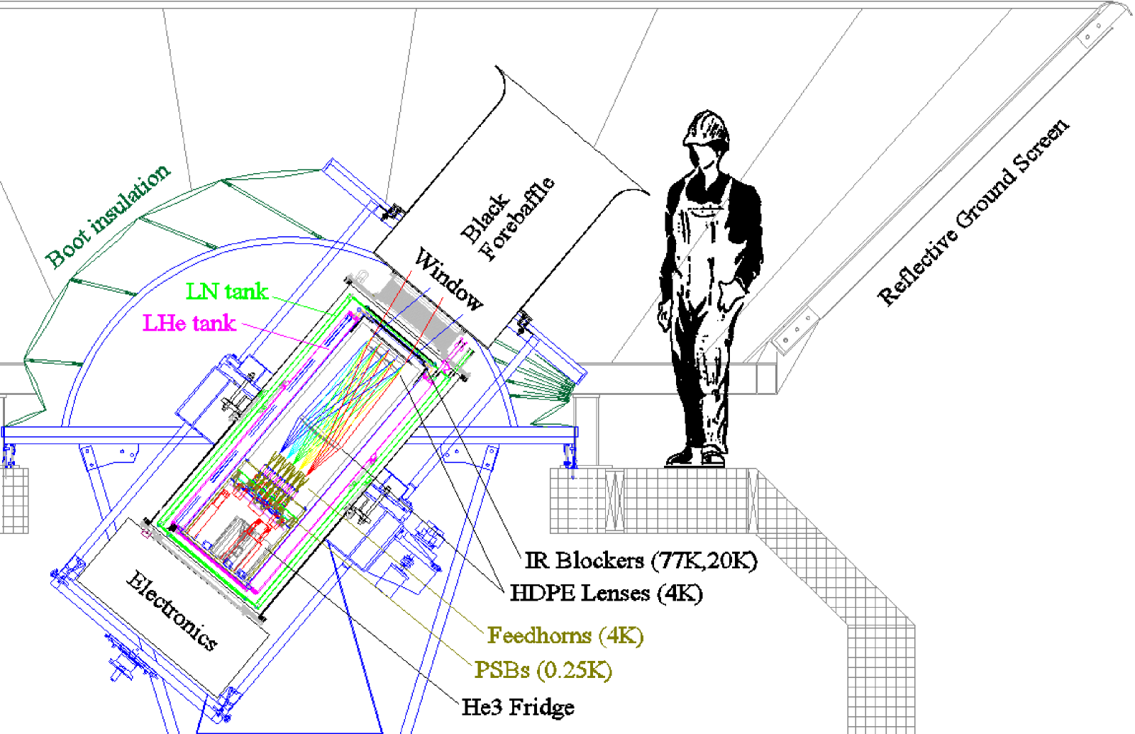
The goal of targeting the sub-K -mode polarization signal that peaks at 2∘ angular scales led to an experiment design optimized especially for sensitivity and control of systematic errors. The design of Bicep and the observation strategy are described in Yoon et al. (2006) and Keating et al. (2003a). Bicep (Figure 1) is a compact on-axis refractor with 49 pairs of polarization-sensitive bolometers (PSBs; Jones et al., 2003) operating in atmospheric transmission windows near the CMB peak at 100 and 150 GHz with and beams, respectively (Table 1). We observe in two frequency bands to differentiate between the spectra of CMB anisotropies and sources of potential Galactic foreground contamination. The Amundsen-Scott South Pole Station, at an elevation of 2800 m, was chosen for its atmospheric transparency, stable weather, and constant availability of an excellent observing field on the sky. Achieving one degree resolution at 2–3 mm wavelengths requires only a 25 cm aperture, which is compatible with a compact forebaffle and simple implementation of calibration measurements.
The bolometers use neutron transmutation doped (NTD) germanium thermistors to measure the optical power incident on a polarization-sensitive absorber mesh. After adjusting for relative responsivities, orthogonal PSBs within a pair are summed or differenced to obtain temperature or polarization measurements. Because the orthogonal PSBs observe the CMB through the same optical path and atmospheric column with nearly identical spectral passbands, systematic contributions to the polarization are minimized.
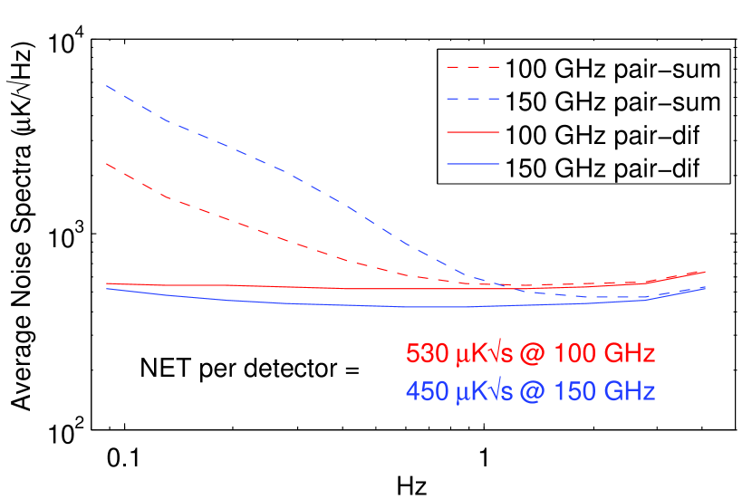
| Band Center | Bandwidth | Beam FWHMa | PSBs | NETb Per Detector |
| 96.0 GHz | 22.3 GHz | 0.93∘ | 50 | 530 K |
| 150.1 GHz | 39.4 GHz | 0.60∘ | 48c | 450 K |
| a Full width at half maximum, average over all the beams. | ||||
| b Noise equivalent temperature; see §4. | ||||
| c After the first year, two of the 150 GHz pairs were converted to 220 GHz. | ||||
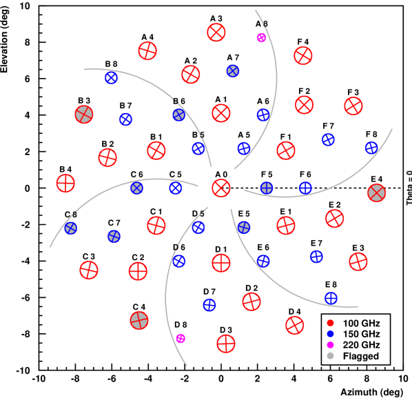
The PSB layout on the focal plane (Figure 2) was chosen so that a 180∘ rotation about the boresight completely exchanges the polarization coverage on the sky. At the end of the first year, in 2006 November, we added prototype 220 GHz feedhorns in place of two of the 150 GHz ones along with the appropriate filters. We also replaced four bolometers because of their slow temporal response, high noise level, or poor polarization efficiency. We have omitted these and other problematic PSB pairs from CMB analysis for each observing year. After this refurbishment, Bicep remained cold and operated without interruption until the completion of the observations in December 2008.
 |
1.2. Observing strategy
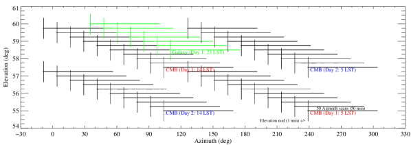
With an instantaneous field of view spanning 18∘, Bicep maps an 800 deg2 field daily by scanning the boresight in azimuth over a 64∘ range at 2.8∘/s with hourly steps in elevation from 55∘ to 60∘. At each elevation step, the telescope completes 50 back-and-forth azimuth scans, or 100 “half-scans,” making up a “scan set.” The scan speed was selected so that our target angular scales ( 30–300) appear at 0.1–1 Hz, above a significant portion of the atmospheric noise, while limiting motion-induced thermal fluctuations at the detectors.
Bicep operates in a 48 sidereal-hour observing cycle (Figure 3), with each cycle at one of the four fixed boresight rotation angles . A rotation about the boresight exchanges the polarization coverages on the sky, providing two independent pairings of angles, each with complete polarization coverage per overlapped sky pixel. The two sets rotated by 180∘ also help to average down systematic effects like differential pointing.
Each 48-hr cycle begins with 6 hours allocated for recycling the refrigerator, filling liquid nitrogen (every 2 days) and liquid helium (every 4 days), and performing optical star pointing calibrations along with a mount tilt measurement. The CMB field is completely mapped once each day in two 9-hr blocks, with the scan order of the upper and lower halves of the elevation range switched such that the azimuth ranges for the two days are offset. Differencing the first and second days of a given 48-hr observing cycle tests for potential azimuth-fixed contamination. Overlapping coverage of the sky from detectors with various polarization orientations is created by scanning in azimuth, stepping in elevation, and rotating the telescope with respect to the boresight every 2 days.
Each scan set at a given elevation is fixed with respect to a given azimuth range instead of tracking the field center over the hour-long period. This scan strategy allows for a straightforward removal of any azimuth- or scan-synchronous contamination. For each scan set and each of the two scan directions, the entire timestream is simply binned in azimuth to form a template signal which is subtracted from each half-scan.
Relative detector responsivities are measured at the beginning and end of each 1-hr fixed-elevation scan set by fitting the detector response to a small change in line-of-sight airmass (“elevation nods”), described in § 3.1.2.
 |
1.3. Collected data and observing efficiency
The Bicep mount was installed at the South Pole in 2005 November, the cryostat was first cooled in December, and the instrument captured first astronomical light a month later. Following calibration measurements and tests of the observing strategy, Bicep began CMB observations in 2006 February. The instrument operated nearly continuously until 2008 December, when it was decommissioned to prepare for its replacement by Bicep2 on the same mount, planned for late 2009.
Excluding any incomplete 9-hr observing blocks, Bicep acquired 180 days of CMB observations during 2006, in which a significant fraction of the observing season was devoted to calibration measurements. The amount of CMB observations increased to 245 days in 2007 and a similar amount in 2008. Although there is no evidence for Sun contamination during the summer, we restrict our CMB analysis to data taken during February–November.
The first 2.5 months of data in 2006 were excluded from the current analysis because a different scan strategy was being investigated at this time. As a coarse weather cut, we have excluded 9-hr blocks if the relative gains derived from elevation nods vary by more than 20% rms, averaged over the channels. This criterion cuts clear outliers in the distribution of atmospheric instability. After these cuts, 117 days in 2006 and 226 days in 2007 remain for our baseline CMB analysis (Table 2).
Furthermore, 3% of PSB pair timestreams are omitted due to cosmic ray hits, glitches, or 3% mismatch in the relative gain measured at the beginning and end of each 1-hr scan set. Accounting for the 75% scan efficiency and the scheduled calibration routines, the net CMB observing efficiency is 60% during the CMB observing blocks and 45% overall during each 2-day cycle.
| Year | PSB Pairs: used (total) | Observing Days: | Integration | |
|---|---|---|---|---|
| 100 GHz | 150 GHz | used (total) | Timea | |
| 2006 | 19 (25) | 14 (24) | 117 (180) days | 4.5 s |
| 2007 | 22 (25) | 15 (22) | 226 (245) days | 8.8 s |
| a Based on 18 hours per day of CMB observation at 60% net observing efficiency. | ||||
2. Calibration goals and systematic error simulation
To process the timestreams into co-added polarization maps with systematic errors tolerable for our target sensitivity, an accurate characterization of the detectors and their beams is essential. Imperfections in the experiment and its characterization can result in false -mode polarization signal. Many of these systematic effects depend in a complex way on the scan strategy, so analytic estimates of the impact of an instrumental uncertainty on the final power spectra serve only as a rough guide. Using the actual analysis pipelines, we have simulated the most significant instrumental uncertainties to establish benchmarks for how precisely each property must be measured. The results are summarized in Table 3. Calibration uncertainties that affect only the power spectrum amplitudes, but do not cause false polarization signals, are summarized in Table 4 and discussed in the last paragraph of this section.
We are most concerned with systematic errors that mix temperature anisotropy and -mode polarization signals into -mode polarization. Instrumental properties that must be characterized are discussed in detail in the next section. The response of a PSB to radiation characterized by Stokes {}, which are functions of frequency and direction , can be modeled as:
| (1) | |||||
where is the polarization orientation angle of the PSB, is the cross-polarization response, is the beam function, is the spectral response, is the effective antenna area, is the responsivity at 0 Hz, is noise, and is the time-domain impulse response associated with the detector’s frequency transfer function. The temporal response function of each bolometer must be measured to deconvolve it from the raw timestream. Then the relative gain within each PSB pair must be determined for differencing. Since we derive relative gains from the atmospheric signal in elevation nods, we must verify that the spectral response of each PSB pair is well matched. In addition, the polarization differencing requires that the two PSBs have well matched beam shapes and pointing. Finally, construction of the polarization map requires the knowledge of the polarization orientations of the PSBs and the telescope pointing.
We established our calibration benchmarks based on Bicep’s design goal to be capable of measuring polarization down to levels corresponding to a tensor-to-scalar ratio without being limited by systematic effects. At , the -mode polarization power spectrum, , would have a peak amplitude of = 0.007 K2 at = 70–110. The benchmarks for the instrumental properties and characterization correspond to the values that result in spurious -mode signal at the level of in the simulations.
The simulation procedure uses the same data processing pipelines as the main CMB power spectrum analysis, and is basically identical to the signal-only simulations used in determining the -space filter function. We verified the simulation results using our two independent pipelines: one using QUaD’s pseudo- estimator on a flat sky, and the other using Spice (Chon et al., 2004) on a curved sky.
We begin with a CDM model generated by CAMB (Lewis et al., 2000), using cosmological parameters derived from 5-year data (Hinshaw et al., 2009) and . From this model, we generate an ensemble of simulated CMB skies using synfast (Górski et al., 2005). We then simulate observations of the Bicep field on these synfast skies using pointing data from the actual scan patterns. We vary instrumental parameters for the PSB pairs with a distribution across the array corresponding to the given uncertainty, but constant in time. We have assumed random distributions, although the differential beams could have a pattern across the focal plane resulting in more or less false signal. For differential pointing, we use the actual measured quantities in the simulations.
| Instrument Property | Benchmarka | Measured | Measurement notes | Reference |
| Relative gain uncertainty: | 0.9% | Upper limit, rms error over the array.b | §3.1 | |
| Differential pointing: c | 1.9% | 1.3% | Average, each repeatedly characterized to 0.4% precision.d | §3.2 |
| Differential beam size: | 3.6% | % | Upper limit, rms over the array. | §3.2 |
| Differential ellipticity: | 1.5% | % | Upper limit, rms over the array. | §3.2 |
| Polarization orientation uncertainty: | 2.3∘ | Upper limit, rms absolute orientation error over the array. | §3.3 | |
| Telescope pointing uncertainty: | 5′ | 0.2′ | Fit residual rms in optical star pointing calibration. | §3.4 |
| Polarized sidelobes (100, 150 GHz) | -9, -4 dBi | -26, -17 dBi | Response at 30∘ from the beam center. | §3.5 |
| Focal plane temperature stability: | 3 nK | 1 nK | Scan-synchronous rms fluctuation on 100 time scale. | §3.6 |
| Optics temperature stability: | 4 K | 0.7 K | Scan-synchronous rms fluctuation on 100 time scale. | §3.6 |
| a Benchmarks correspond to values that result in a false -mode signal of at most . For , all benchmarks would be lower by . | ||||
| b If relative gain errors are detected, we anticipate removing their effects in future analyses using a CMB temperature template map. | ||||
| c = {0.39∘, 0.26∘} at {100, 150} GHz. | ||||
| d This measurement of differential pointing could be used in future analyses to remove the small predicted leakage of CMB temperature into polarization maps. | ||||
To simulate the coupling between non-ideal beams and the sky, we follow the formalism in Bock et al. (2008). A PSB timestream sample is expressed as a convolution of the beam with a second-order Taylor expansion of the sky signal around the pointing center—the first and second derivatives of simulated , , and maps are calculated with synfast. Using this technique, the beam convolution can be simulated quickly while using the exact scan trajectory of each detector, which is essential in quantifying the beam mismatch effects, as these depend on the scan strategy and on the combination of detectors with different characteristics. This formalism also allows simulation of the impact of uncertainties in the knowledge of PSB orientations and cross-polarization response.
The simulated observation is performed at each of the 4 boresight rotation angles and with the appropriate instrument configuration for each observing year. The simulated signal-only timestreams are fed through the pipelines to be filtered and co-added into maps with exactly the same weights as with the real data. A baseline set of spectra are computed without any simulated errors to (1) determine the amount of - leakage due to timestream filtering and any other effects intrinsic to the pipeline, and (2) obtain the transfer functions to be applied to the raw spectra.
The power spectra of maps made with simulated errors are compared with those without any errors, and any differences—in particular, excess -mode polarization power that has leaked from or —are attributed to the systematic errors. The simulations are performed with at least 10 realizations of input CMB maps.
Table 3 summarizes the instrument properties and benchmark levels for their characterization, as well as the results of measurements described in the next section. Each instrumental property has been characterized to a level of precision at least comparable to the benchmark and in most cases much better.
Finally, some calibration uncertainties affect only the scaling of the spectra but do not result in spurious polarization signals (Table 4). These effects can be calculated analytically, and are described in the next section. We set the benchmark for each of these uncertainties such that the contribution to the calibration of power spectrum amplitudes is , a standard easily met by our instrument characterization.
affecting the power spectrum amplitudes only
| Calibration Quantity | Benchmarka | Measured |
|---|---|---|
| Absolute gain | ||
| Cross-polarization response | ||
| Relative polarization orientation | ||
| a Benchmarks correspond to 10% uncertainty in the polarization power spectrum | ||
| amplitude. | ||
3. Instrument characterization
We use the benchmarks found in the previous section to guide our program to characterize the instrumental performance. To reach the required level of precision, we designed and implemented a number of techniques for the calibration measurements. This section describes the measurements for relative gain calibrations, beam characterization, polarization calibration, telescope pointing, far sidelobes, and thermal stability and compares the results with the benchmark values leading to a reference level of uncertainty in power spectrum. The characterization of the instrument noise and its implications for uncertainty in the power spectrum is discussed in §4. All the instrumental quantities have been measured with sufficient accuracy for the sensitivity achieved with the first 2 years of data.
3.1. Relative detector gains
Polarization measurement with Bicep relies on PSB pair differencing. The relative gains within each pair must be accurately determined to prevent unpolarized signal from leaking into the polarization measurement. The relative amplitudes of the CMB temperature and polarization anisotropies place stringent requirements on the relative gain calibration of the differenced detectors. Simulations of relative gain errors suggest that the level of false polarization depends strongly on how gain errors are distributed across the PSB array. With the best estimated distribution of the measured gain uncertainties described in §3.1.2, the simulations indicate that relative gains need to be accurate to 0.9% rms to limit the leakage of CMB temperature anisotropy into -mode power at a level corresponding to .
We correct for relative gain differences in two steps, first by deconvolving the temporal transfer function of each PSB to account for frequency-dependent gains, and then by correcting for the DC gains through elevation nods. Since elevation nods use the atmospheric emission, which has a different emission spectrum than the CMB temperature fluctuations, the spectral response of each PSB in a pair must be precisely matched. We measured the detector transfer functions each year, calibrated the DC gains hourly with elevation nods, and made spectral response measurements once before deployment and once in the field. The following subsections describe the measurements of temporal transfer function, DC responsivities, and spectral response. The transfer functions for each pair were measured to within 0.3% uncertainty and elevation nod relative gains to within 1.1% rms uncertainty over the PSB pairs. While the current upper limit on the possible relative gain errors slightly exceeds the 0.9% benchmark for , this effect is not significant for the 2-year CMB results; furthermore, if a significant signal was detected it could be corrected with a more sophisticated analysis.
3.1.1 Temporal transfer functions
Analysis of the time series from each detector begins by deconvolving the temporal response using the measured frequency-domain optical transfer function of the detector. Since the transfer function is proportional to the gain of the detector as a function of frequency, it directly affects the relative gains of a PSB pair to be differenced. The relative transfer functions must thus be measured with errors below the 0.9% benchmark set for the relative gains.
At the nominal scan speed of /s in azimuth at 60∘ elevations, our target angular scales of 30–300 fall into the frequency band of approximately 0.1–1 Hz. Since the elevation nods described in the following section are sensitive to relative fluctuations at 0.02 Hz, the transfer functions were measured down to 0.01 Hz.
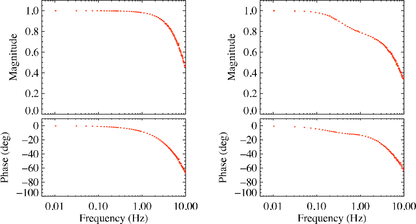
The primary measurement technique involved analyzing the step response to a fast-switched square-wave source (Gunn oscillator or broadband noise source) operating at 0.01 Hz, while under optical loading conditions representative of CMB observations (Figure 4). Possible dependence on background loading and detector non-linearity were explored by repeating the measurement with extra loading from sheets of emissive foam placed in the beam in combination with different signal strengths. The ratio of the Fourier transforms of the time-domain detector response and of the input square wave were averaged for each detector to obtain the transfer function. The measured transfer functions for a representative and anomalous PSBs are shown in Figure 5; they were stable against different combinations of loading and signal levels.
The relative gain uncertainty due to measurement uncertainty is found to be 0.3% over the frequency range of 0.01–1 Hz. The measured transfer functions fit the following model as a function of frequency ,
| (2) |
where are time constants and is the fractional amount of a slow additive component. However, we measured the transfer functions with sufficiently high signal-to-noise ratio so that they could be directly inverse Fourier transformed to define the deconvolution kernels. The median time constants were ms and ms, and is generally 100–200 ms with typically 0.05. From the first observing year, 6 channels at 150 GHz were excluded from CMB analysis due to excessive roll off between 0.01 and 0.1 Hz (large and ). Two of the worst were in a single PSB pair and were replaced at the end of the year.
Between the first two observing years, the transfer function measurements generally agreed to within 0.5% rms across the signal band. Two exceptions were excluded from the first year CMB data where the transfer functions were less well constrained at low frequencies. Details of the measurements and analysis are in Yoon (2007).
3.1.2 Relative responsivities
Relative gains are derived from elevation nods performed at the beginning and end of every 1-hr constant-elevation scan set (Figure 3). The telescope scans in elevation with a rounded triangle wave pattern over a range of , varying the optical loading by 0.1 K due to the changing line-of-sight air mass. The bolometer responses are fit to a simple air mass model of atmospheric loading versus elevation, csc(), to derive the relative gains across the array.
The elevation nod is performed slowly over 50 s to limit thermal disturbances on the focal plane. During the nod, the diagnostic “dark” PSBs not illuminated through the feedhorns exhibit systematic voltage responses (also seen in the focal plane thermistors but not in the resistor channels) that are 0.4% of the typical responses of the illuminated PSBs, indicating thermal contamination at this level. To reduce the effect of the thermally-induced signals, the two elevation nods for each scan set are performed in opposite patterns (up-down-return and down-up-return) and the average response is used. While the two patterns result in a small systematic difference in the individual gains, the PSB pair relative gains are consistent to within the measurement noise of 0.3% rms.
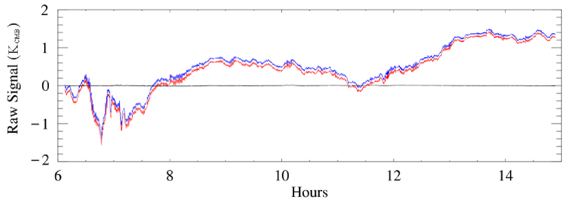
PSB pair differencing is able to remove common-mode atmospheric fluctuations, and the relative gains are very stable (Figure 6). Even over a time scale of months, the relative gains are stable with 1% rms measurement noise and exhibit no systematic variation with the optical loading. Relative gains have also been derived from correlating timestream atmospheric fluctuations within PSB pairs, and although these have greater statistical uncertainties the results are consistent with the elevation nods to within 3%.
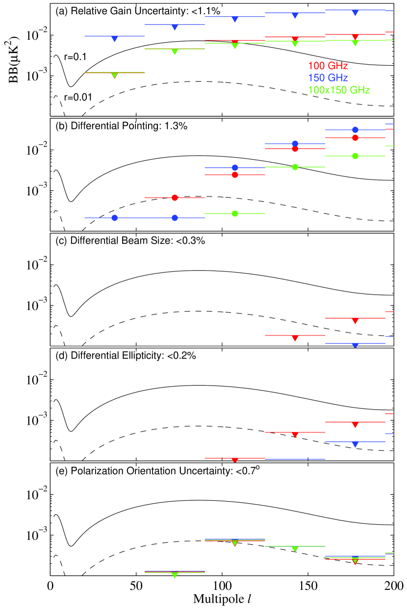
As an additional method to track gain variations, an infrared source supported by a foam paddle is swung into the beam to inject a signal of very stable amplitude, as described in Yoon et al. (2006). It produced a very repeatable (0.2% rms) response between the beginning and end of the 1-hr scan sets and also showed that the individual gains are stable with 1% rms across the full elevation range. However, because of the 3 K optical loading introduced by the swing arm and unknown polarization of the infrared source, the relative gains from the flash calibrator have not been used for pair-differencing.
To quantify the level of leakage of the CMB temperature anisotropy into pair differences, the individual PSB pair-sum and pair-difference maps were cross-correlated. This analysis performed on the yearly maps from the first 2 years showed no statistically significant evidence for relative gain errors in the data and placed an upper limit of 1.1% rms on the angular scales of interest. There is weak evidence that a small subset of PSB pairs, especially at 150 GHz, have excess sum-difference correlations. With the full 3-year data set, we anticipate placing tighter constraints on the gain uncertainties. The power spectra of spurious -mode polarization due to the best-estimate distributions of 1.1% rms relative gain errors are plotted in Figure 10a. Although these upper limits exceed the signal for on some scales, especially for 150 GHz, this systematic effect is still well below the statistical error in the first 2 years of data. If measured, this leakage can be mitigated by projecting out a CMB temperature anisotropy template from the polarization maps.
The measured individual gains are scaled for each 1-hr scan set such that the mean response of the detectors in each frequency band is constant. Finally, the absolute gains for converting the detector voltage into CMB temperature units are derived by cross-correlating maps of CMB temperature anisotropy measured by Bicep and . As described in detail in Chiang et al. (2010), the Bicep map (in volts) and “Bicep-observed” maps (in KCMB) are identically smoothed and filtered, and we compute the absolute gain for each of the frequency bands from cross-correlations in multipole space. Within the multipole range of 56–265, is nearly flat, and the average is used as a single calibration factor for each frequency band. We take the standard deviation of 2% to be a conservative estimate of the absolute gain uncertainty in CMB temperature units. The results are consistent with those from the dielectric sheet calibrator (described in §3.3), which can provide a real time absolute calibration with a 10% uncertainty.
3.1.3 Spectral response
As described above, the relative gain calibration of a PSB pair is based on the relative response of the detectors to the change in atmospheric loading from a small nod in elevation. Because the temperature derivative of the CMB and the atmospheric emission have different spectral shapes, the relative gain chosen to match the response to elevation nods may not be optimal for the rejection of CMB temperature fluctuations.
The spectral response of each channel was measured using two separate polarized Fourier Transform Spectrometers with a maximum resolution of 0.3 GHz, once in the lab and once in the field. Within each frequency band, the spectra were very similar from channel to channel (average spectra shown in Figure 7), and the upper limit on the expected relative gain errors due to spectral mismatch was roughly 1% rms over the array. This current upper limit does not rule out spectral mismatch as a source of possible relative gain errors in the small subset of PSB pairs.
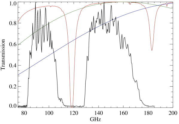
In addition to the main band, we verified that there is no significant response at higher frequencies due to leaks in the low-pass filters. High-pass thick grill filters with cut-off frequencies of 165 and 255 GHz were used in front of the telescope aperture one at a time and the response to a chopped thermal source was measured. 150 GHz channels showed no sign of leaks beyond 255 GHz down to the noise floor at dB, while 100 GHz channels exhibited leaks at dB level at 255 GHz. The magnitude of this small (0.3%) leak was consistent between the PSBs in each pair, so the effect on relative responsivities is expected to be negligible.
3.2. Beam characterization
Mismatch in the beams of a PSB pair can result in a false polarization signal from unpolarized temperature fluctuations. Beam mismatches can also lead to the mixing between -mode and -mode polarization. The difference between two nearly circular beams can be decomposed into three quantities corresponding to monopole, dipole, and quadrupole differentials: differential beam size , differential pointing , and differential ellipticity , where are the Gaussian beam sizes of the first and second PSBs in a pair, is the average beam size, and are the centroid coordinates. We define ellipticity as , where are widths of the major and minor axes, respectively. Beam size and ellipticity differences are sensitive to the second spatial derivative of the temperature field, while pointing offset is also sensitive to the temperature gradient.
For Bicep’s focal plane layout and scan strategy, simulations show that differential beam size, pointing, and ellipticity of 3.6%, 1.9%, and 1.5% rms over the array, respectively, will result in spurious -mode signal at the level. The effect of differential pointing was simulated using the measured magnitude and direction of beam offsets with the expected amount of false power scaling as the square of the magnitude. Differential beam size was simulated by introducing a random distribution of beam size differences in PSB pairs, while keeping the average beam size the same. Similarly, differential ellipticity was simulated by making the beam of every PSB elliptical by a small randomized amount such that the pairs have ellipticity differences of the given rms while keeping the beam sizes the same. The measurements described below indicate that the major axes tend to be more azimuthal with respect to the optical axis than radial, and the major axes of paired PSB beams tend to align within 15∘ rms of each other. Therefore, the major axes in the simulations were varied around the azimuthal direction by 10∘ rms to roughly simulate the observed alignment trend within each pair. Analytic calculations show, and these simulations verify, that the expected false power scales as the square of differential beam size or ellipticity and as the fourth power of the beam size (Shimon et al., 2008).
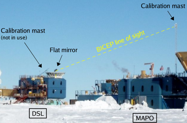
The beams were mapped by raster scanning a bright source at various boresight rotation angles. The far field of the telescope is about 50 m from the aperture, which permitted measurements in a high bay prior to telescope deployment as well as with the instrument installed at the South Pole. In the high bay, a thermal blackbody source was used at a 40 m distance, consisting of a liquid nitrogen temperature load behind chopper blades covered with ambient temperature absorber. At the South Pole, a temporary mast was installed on the rooftop outside of the fixed ground screen, allowing us to position a source at 60∘ elevation 10 m away. For a truly far-field measurement, an additional mast was installed on the roof of the Martin A. Pomerantz Observatory (MAPO), at a distance of 200 m, and a flat mirror was temporarily mounted on top of the telescope to direct the beams down to allow the observation of the distant mast as well as low elevation astronomical sources (Figure 8). The sources used included an ambient temperature chopper against the cold sky, a broadband noise source, the Moon, and Jupiter. The broadband noise source is an amplified thermal source that is ideal for probing low-level effects.
The measured beams are well fit with a Gaussian model, typically resulting in 1% residuals in amplitude. The fitted centroids are repeatable to about 0.02∘, although the accuracy of the absolute locations is currently limited by uncertainties in parallax and pointing corrections while using the flat mirror. The average measured FWHMs are 0.93∘ and 0.60∘ for 100 and 150 GHz, respectively, about 5% smaller than predicted from physical optics simulations. The beam widths are measured to 0.5% precision and vary by 3% across the array. The beams have small ellipticities of 1% at 100 GHz and 1.5% at 150 GHz.
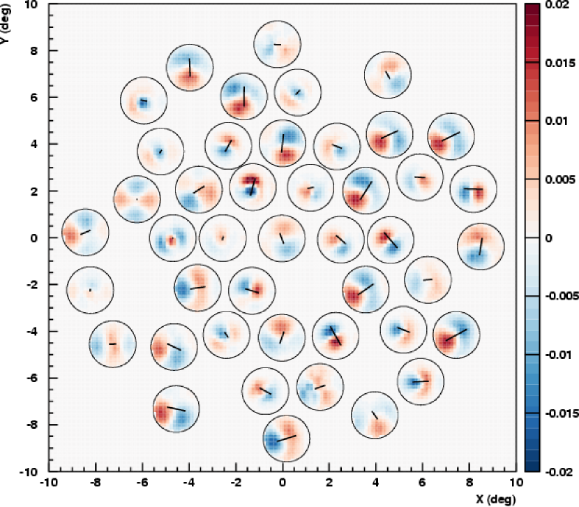
The largest beam mismatch effect is a pointing offset that gives rise to dipole patterns in many of the differenced beams (Figure 9). The median differential pointing offset is 0.004∘ at both 100 and 150 GHz, and is on average 1.3% of the beam size . The offsets were repeatable between observations of both the broadband noise source and the Moon to within the measurement uncertainty of 0.4% of .
Simulated observations with the measured pointing offsets indicate a false with an amplitude comparable to the spectrum (Figure 10b), although well below the noise level of the initial 2-year data analysis. With the magnitude and direction of the pointing offsets measured precisely, the resulting leakage of CMB temperature gradients into polarization can be estimated and accounted for in future analysis. Differential beam size and ellipticity are not measured with significance; the measured upper limits of 0.3% and 0.2% rms, respectively, are negligibly small (Figure 10c,d).
3.3. Polarization orientations and efficiencies
To construct accurate polarization maps from PSB timestreams, we must know the polarization orientation angle and cross-polarization response of each PSB. Accurate orientations must be used in map making to prevent rotation of -mode polarization into false -mode. Cross-polarization response determines the polarization efficiency , which affects the amplitude scaling of the power spectrum. We developed experimental techniques to measure these quantities by injecting polarized radiation into the telescope aperture at many different angles with respect to the detectors. The phase and amplitude of each PSB’s response determine and , respectively. This section discusses the calibration benchmarks for these quantities and describes three measurement techniques and their results. The absolute PSB orientations were measured to within and relative orientation to within , and was measured to within 0.01.
Angles of the PSBs can vary from their design orientations due to the limited mechanical tolerances with which they are mounted. The deviation from perfect orthogonality of a pair simply reduces its efficiency for polarization; however, an error in the overall orientation of the pair can lead to rotation of -modes into -modes. With the expected fractional leakage being sin(2), the 1 K -modes at can rotate into false -modes at the level of 0.08 K if the orientation measurement is off by 2.3∘. This benchmark and the expected scaling were verified by simulations of systematic orientation offset of all the PSBs. The calibration procedure was designed to determine the polarization orientations to within a degree.
Another factor, though less important, is that the PSBs are not perfectly insensitive to polarization components orthogonal to their orientations, effectively reducing the polarization efficiency to . To achieve 10% accuracy in the amplitudes of the polarization power spectra, which are proportional to , our goal was to measure cross-polarization responses to better than 0.026.
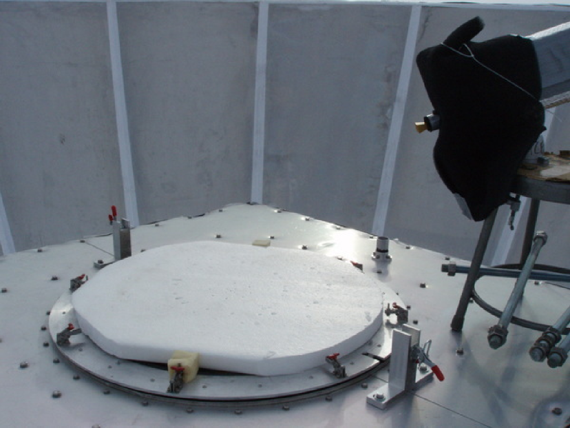
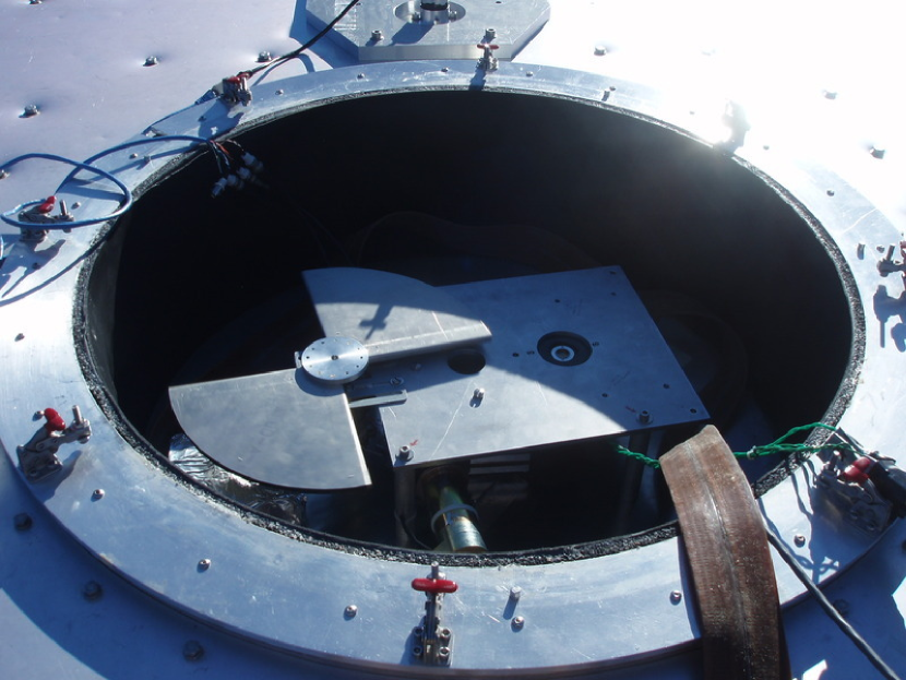
The polarization orientations were measured using a rotatable dielectric sheet (Figure 11), modeled after the one used by POLAR (O’Dell, 2002). A small partially polarized signal of known magnitude is created by using an 18-m polypropylene sheet in front of the telescope aperture oriented at 45∘ to the optical axis. The sheet acts as a beam splitter transmitting most of the sky radiation but reflecting a small polarized fraction of the radiation from an ambient load perpendicular to the beam. The polarized signal is small compared to the unpolarized sky background so that it can provide an absolute responsivity calibration in optical loading conditions appropriate for normal observations. The ambient load is made of a microwave absorber lining inside an aluminum cylinder surrounding the beam splitter. The absorber is covered with a 1/8” thick sheet of closed cell expanded polyethylene foam exactly as in the forebaffle (described in §3.5), the combination of which has 95% emissivity at 100 GHz.
We use this polarization calibrator by putting it in the place of the forebaffle and fixing it to the azimuth mount. With the telescope pointed at zenith, rotating the device with respect to the cryostat modulates the polarization signal for each detector while keeping the beams stationary with respect to the sky. The off-axis beams see complicated, but calculable, deviations from the nominal sinusoidal modulation (Figure 12). This setup produces a partial polarization of amplitude proportional to , the temperature difference between the ambient load and the sky loading. With an 18-m polypropylene film and a typical temperatures of = 220 K and = 10 K, the signal amplitude is 100 mK at 100 GHz and 250 mK at 150 GHz, small enough to ensure that the bolometer response remains linear.
The measurements were performed several times throughout each observing year and produced repeatable results for the individual PSB orientations with 0.1∘ rms. The relative orientation uncertainty of results in negligible absolution calibration error. The PSB pairs were found to be orthogonal to within 0.1∘, and together were within 1∘ of the design orientations shown in Figure 2. PSB orientation measurements performed before and after the focal plane servicing (2006 November) show a possible discrepancy, corresponding to an average of 1.0∘ global rotation. We therefore conservatively assign a 0.7∘ rms uncertainty in the absolute orientation for each year. This absolute orientation angle accuracy is sufficient for measuring (Figure 10e).
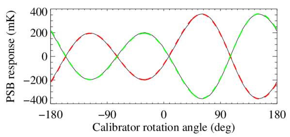
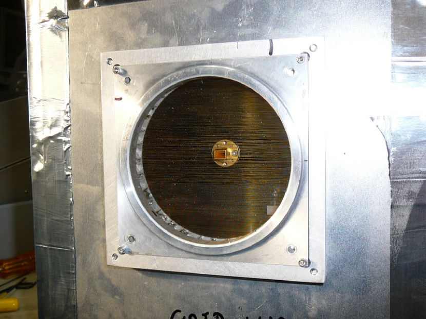
The cross-polarization responses were measured using two methods that also independently confirmed the absolute orientation measurement. One method used a rotatable wire grid in front of the telescope window with a chopper modulating the polarized load through a small aperture between the ambient absorber and the cold sky (Figure 13). Fitting a sinusoid to the individual PSB response as a function of the wire grid angle gives the polarization efficiency and orientation. The measurements for all three years gave cross-polarization response values with a distribution . One 150 GHz bolometer was omitted from analysis for having an and was replaced at the end of the first year.
The other method used a modulated broadband noise source with a rectangular horn behind a wire grid, mounted on the mast 200 m away (Figure 14). This source was raster scanned by each of our beams with 18 different detector orientations with respect to the wire grid, fitting a 2-dimensional Gaussian to each raster. The measured cross-polarization responses were slightly lower with a median of . Based on the scatter against the results from the first method, we assign an uncertainty of , which translates to 4% uncertainty in the polarization power spectrum amplitudes.
3.4. Telescope and detector pointing
Pointing errors greater than 1% of the beam size could contaminate the -mode spectrum at the level (Hu et al., 2003). Since the amount of spurious power scales as the square of the pointing error, the benchmark would correspond to 0.3, or 5′ for Bicep. This benchmark was verified to be conservative by simulating a 5′ rms shift in boresight pointing every 10 elevation steps in one of our simulation pipelines and finding negligible spurious signal compared to the signal. An optical star pointing camera is used to measure the telescope boresight pointing model with uncertainties more than an order of magnitude smaller than required to achieve our benchmark.
An accurate derivation of the sky coordinates from the telescope encoder readings requires a precise knowledge of the state of the mount, including axis tilts, encoder offsets, and flexure. Encoder data for the three mount axes are recorded synchronously with the bolometer timestreams and corrections to the raw pointing data are applied during map making using a pointing model. The pointing model is established using a compact optical star-pointing camera with a 2′′ resolution mounted beside the main window on top of the cryostat and co-aligned with the boresight rotation axis. There are 10 dynamic parameters: AZ axis tilt magnitude and direction, EL axis tilt, the 3 encoder zeros, amount of telescope flexure cos() and sin(), and magnitude and direction of the collimation error of the pointing camera itself. A complete characterization of these parameters requires the observation of at least 20 stars. To establish a pointing model during the Antarctic summer, the pointing camera was designed to be sensitive enough to detect magnitude +3 stars in daylight. For maximum contrast against the blue sky, we used a sensor with enhanced near-infrared sensitivity111Astrovid StellaCam EX with EXview HAD CCD, http://www.astrovid.com/prod_details.php?pid=7 and an infrared filter cutting off below 720 nm. We used a 100-mm diameter lens that was color-corrected and anti-reflection coated for 720–950 nm. Its 901-mm focal length results in a small 0.5∘ field of view to keep the sky background low. Careful adjustments of the CCD camera and the mirrors reduced the optical camera’s collimation error to 2.4′. During our first Antarctic summer season, we successfully captured 26 stars down to magnitude +2.9 in an elevation range of 55∘–90∘.
Optical pointing calibrations were performed every two days during the refrigerator cycles, weather permitting, as well as before and after each mount re-leveling. In each run, the telescope is pointed at 24 stars at boresight rotation angles of , , and , and the azimuth and elevation offsets required to center each star are recorded. The pointing data are fit to an 8-parameter model (it has not been necessary to fit for telescope flexure) with typical residuals of rms. The pointing model has been checked by cross-correlating the CMB temperature anisotropy patterns between the pointing-corrected daily maps and the cumulative map; no systematic offsets or drifts are detected.
In parallel with the optical pointing calibration, the tilt of the telescope mount is monitored every two days using two orthogonal tilt meters mounted on the azimuth stage. We observed seasonal tilt changes of up to 0.5′ per month, possibly due to the building settling on the snow, and typically re-leveled the mount before the tilt exceeded 1′.
Finally, to co-add maps made with different PSB pairs, the actual locations of all the beams relative to the boresight must be determined. This was accomplished by first making a full season co-added map of the CMB using the design locations and then cross-correlating the temperature anisotropy pattern with single detector maps for each of the four boresight rotation angles to adjust the individual beam coordinates. These adjusted coordinates with respect to the boresight were then used to iterate this process until every individual pair map was consistent with the full co-added map. This derivation of the absolute beam locations resulted in an uncertainty of rms, based on the agreement between the first and second years. For Bicep, using the CMB temperature fluctuations proved to be more effective than attempting a similar procedure with Eta Carinae, the brightest compact source accessible.
3.5. Sidelobe rejection
Sidelobes of the telescope beams can pick up emission from the bright Galactic plane and structures on the ground, possibly resulting in contamination of the polarization maps. The ground shields were designed to reject the ground radiation to a level where the contamination is below our target -mode polarization sensitivity. This section describes the ground shield design, the sidelobe measurement, and the possible polarization contamination due to the sidelobes. Bicep’s sidelobes are sufficiently low to enable the measurement of -mode polarization to the level of r=0.01.
Bicep uses two levels of shielding against ground radiation: an absorptive forebaffle fixed to the cryostat and a large stationary reflective shield surrounding the telescope structure (Figure 15), modeled after the POLAR experiment (Keating et al., 2003b). We designed the geometry so that any radiation from the ground must be diffracted at least twice before entering the window in any telescope orientation.
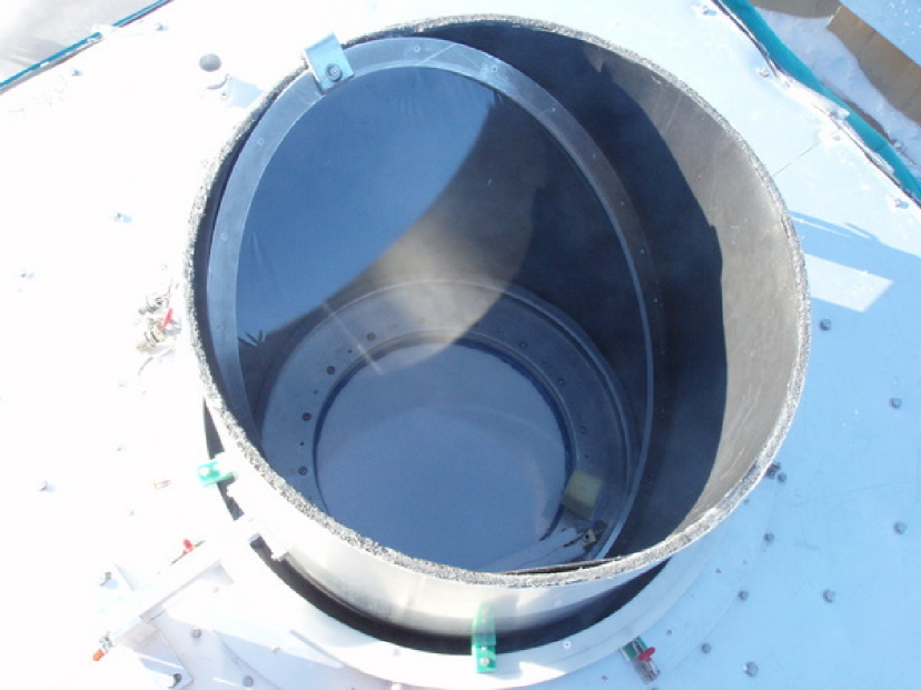
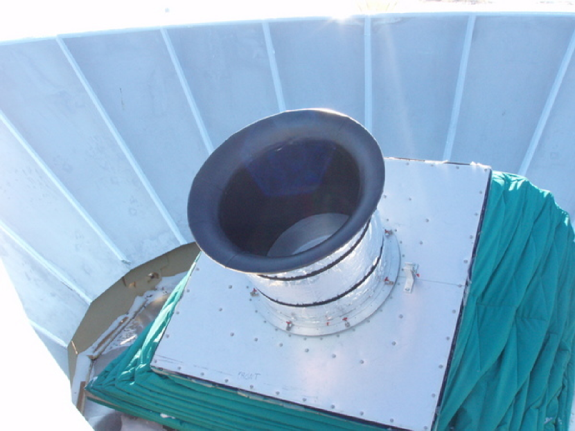
The forebaffle is an aluminum cylinder lined with a microwave absorber to minimize reflected radiation into the telescope. It is wide enough to clear the edge pixel beams, beyond which the Zotefoam222Propozote PPA30, http://zotefoams.com/pages/en/datasheets/PPA30.htm window (Runyan et al., 2003) is expected to scatter 1% of the total power. At Bicep’s lowest nominal CMB observing elevation of 55∘, the forebaffle is long enough to prevent radiation from sources, particularly the Moon, at elevations up to 27∘ from entering the window directly. The forebaffle aperture lip is rounded with a 13 cm radius to reduce diffraction of the diffuse beam sidelobes.
After testing many materials for the microwave absorber, we chose a 10-mm thick open-cell polyurethane foam sheet (Eccosorb HR333http://www.eccosorb.com/america/english/product/40/eccosorb-hr), which had the lowest measured reflectivity of 3% at 100 and 150 GHz when placed over a metal surface (150 GHz results by W. Lu & J. Ruhl 2004, private communication). To prevent snow from accumulating in the porous Eccosorb foam, it is covered with a 1.6-mm thick smooth polyethylene foam (Volara444Volara; Sekisui Voltek, http://www.sekisuivoltek.com/products/volara.php), which is attached with a silicone sealant. The combined Eccosorb HR / Volara stack was measured to reflect 5% of GHz radiation incident at 45∘. The additional loading on the bolometers due to emission from the forebaffle was measured to be 1 KRJ. Since the absorptive baffle is fixed with respect to the detectors, its thermal emission is expected to be stable against the modulated sky signal.
The 2-m tall outer screen prevents the forebaffle lip from seeing the warm ground. The sloped aluminum surface instead reflects any diffuse sidelobes to the relatively homogeneous cold sky. The 8-m top diameter is wide enough so that the diffracted ground radiation will never directly hit the window even when the telescope is at its 50∘ elevation lower limit. The edge of the outer screen is also rounded with a 10 cm radius to reduce diffraction.
The sidelobe response of the telescope, including the forebaffle, was measured using a chopped broadband noise source on the mast m from the telescope aperture. The telescope was stepped in elevation up to 60∘ away from the source in 0.5∘ increments, making one revolution about the boresight and back at each step to measure a radial average of the beam. This measurement was performed with several source attenuations down to below dB to probe the far sidelobes with sufficient signal-to-noise ratio while also measuring the main beam without saturating the detector.
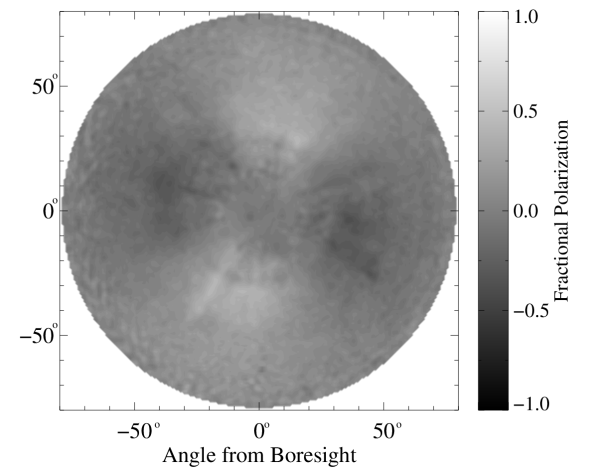
Sidelobe response maps constructed from the gain-adjusted pair differences show that the sidelobes are up to 50% polarized (Figure 16). The individual sidelobe maps can be averaged over boresight rotation angle to obtain a radial profile (Figure 17). Waves polarized parallel to the absorbing forebaffle lip surface are more strongly diffracted than those polarized perpendicular to the lip. This difference appears to be mainly responsible for the polarized response in the sidelobes.

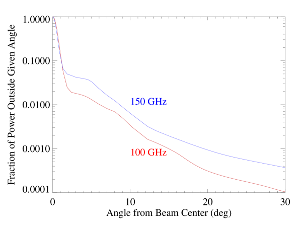
To quantify what fraction of the total power in the beam remains outside of a given angle from the beam center, the net beam profile for horizontal and vertical polarizations was integrated (Figure 18). Less than 0.1% of the power in the beam is left beyond 15∘ and 20∘ of the beam center at 100 and 150 GHz, respectively.
Polarized sidelobes can result in spurious signals by coupling to emission from the Galaxy and the outer ground screen itself. To evaluate the far sidelobe rejection performance, the measured level of polarized response was convolved with a model map of a potential contaminant, and an angular power spectrum was computed in the Bicep field to compare with the spectrum. For the Galactic model, we used the dust emission predicted by Finkbeiner et al. (1999). The resulting -mode contamination was found to be at least 400 times below the level, meaning the measured sidelobes are at least 13 dB below the benchmark. The same exercise was repeated for a conservative model of snow accumulation on the ground screen panels. The contamination was even smaller, with the achieved rejection level at least 23 dB better than the benchmark.
We have also probed potential ground contamination in our data through a jackknife test comparing maps made in different azimuth ranges, and have seen no evidence of ground signal. As mentioned in §1.2, the scan range is fixed with respect to ground during each 1-hr scan set so that subtracting a scan-synchronous template each hour removes any ground-fixed signal.
3.6. Thermal stability
The thermal and optical responsivities of PSBs in each pair are not perfectly matched, so the temperatures of the detector focal plane and the emissive optics must be sufficiently stable to prevent the introduction of scan-synchronous thermal signals. We have measured the thermal responsivity of every bolometer and compared the mismatches with the focal plane temperature stability, which we control with a feedback loop. The thermal stability of both the focal plane and the optics is found to be adequate compared to the benchmark.
The bolometers’ responsivities to the bath temperature are measured by correlating the detector timestreams with the 10 mK drop when the temperature control heater is turned off at the end of each refrigerator cycle. The median thermal responsivity, after converting voltages into CMB temperature units, is 0.8 KCMB/nKFP, and the median mismatch within PSB pairs is 0.08 KCMB/nKFP. Because the pair differential responsivities are distributed randomly in the array, the effects of the mismatch will average out when the maps are co-added. The averaged mismatch over the array, considering both the magnitudes and signs of the thermal response, is 0.025 and 0.001 KCMB/nKFP at 100 and 150 GHz, respectively. To meet the target of 0.08 KCMB at 100, thermal instabilities in the focal plane must then be controlled to better than 3 nK rms.
To mitigate the thermal fluctuation effects, the focal plane temperature is stabilized at 250 mK using a 100 k resistor as a control heater (nominally depositing 0.1 W) in a PID feedback loop with a sensitive NTD germanium thermistor. The PID parameters are set such that no active regulation takes place within the observational signal band of 0.1–1 Hz; only long time-scale drifts are controlled so that the PSB relative gains remain unaffected. The focal plane is equipped with 6 pairs of monitor thermistors spaced evenly around its perimeter. During the first year, the thermal control scheme used a thermistor closest to the thermal strap connected to the refrigerator. To improve the recovery time from major thermal disturbances and other transient events, additional control thermistors were installed near the control heater on the thermal strap at the end of the first year. The rigidity of the thermal straps were improved by using Vespel555http://www2.dupont.com/Vespel/en_US supports to reduce susceptibility to vibrationally induced heating. Along with an increased response speed of the control loop, the temperature stability measured by the focal plane thermistors was improved from the first year to the second.
The temperature stability of the focal plane was found to vary with azimuth scan speed as well as the cryostat orientation about its axis. The stability was investigated under a variety of telescope operating conditions, including scan speeds in a range of /s – /s, and 16 evenly spaced boresight rotation angles. Based on the minimum variance of the scan-synchronous thermistor signals, we selected the 2.8∘/s nominal scan speed and four cryostat orientations about the boresight: . The measured level of thermal fluctuations at the Bicep focal plane was 1 nK rms in the frequency range corresponding to .
Finally, since emission from Bicep’s optics is expected to be largely unpolarized, the main concern with optics temperature drifts is in mis-calibration of PSB pair optical relative gains, which have an upper limit of 1.1% rms, as described in §3.1.2. To limit the pair-difference response to less than 0.08 KCMB, the scan-synchronous optical loading fluctuations must be under 8 KCMB, requiring the optics temperature to be stable to at least 4 KRJ rms (for the 150 GHz band). Scan-synchronous fluctuations averaged over all the individual bolometers for a two month period show 0.7 KRJ rms variation in the frequency range 0.1–1 Hz.
4. Noise properties and modeling
Precise characterization of noise in the Bicep data is crucial for accurately extracting the underlying CMB polarization angular power spectrum. The detector timestreams are dominated by noise which must be modeled and simulated to subtract the noise bias from the resulting power spectra. Precise subtraction is critical because any misestimation results in a systematic error in the power spectrum amplitude. Simulating the effect of a noise misestimate on the final spectrum from the 2-year Bicep data, we find that a overall error in the noise power estimate would result in a bias of . This translates to a benchmark of 1.5% accuracy in CMB temperature units for the pair difference noise simulation. Also, the simulation of noise, along with that of signal, determines the error bars of the CMB power spectra and the constraints on the -mode polarization amplitude. To remove noise bias from the raw power spectra, we simulate signal-free, noise-only timestreams and process them with the same pipeline as the actual data to compute the noise power spectra. This section describes characterization of the noise properties, simulation of noise-only timestreams, and the resulting estimates of the noise bias in the final angular power spectrum. The noise level is consistent with expectations and no significant cross-correlations in noise are observed among pair differences, and the simulated noise has been checked for consistency with the actual noise level in the data.
4.1. Properties of noise: spectra and covariance
To simulate noise-only timestreams with the same statistical properties as the actual data, the noise properties must first be modeled. Because Bicep’s raw timestreams are dominated by noise, we model the noise by simply computing the auto and cross spectral power distributions for detector sums and differences. The signal-to-noise ratio in the timestreams is 0.2% for the PSB pair differences and 1–10% for the pair sums in the 0.1–1 Hz frequency range corresponding to 30–300. The significant CMB signal in the pair-sum timestreams is expected to introduce some error, but we permit this in the present analysis because the uncertainty in noise bias is expected to be much smaller than the cosmic variance in the temperature power spectrum. The present noise model accounts for correlations among all the detectors in the focal plane, but does not attempt to include correlations between half-scans or between orthogonal Fourier modes within each half-scan.
PSB pair sums and differences are modeled and simulated after the removal of a third-order polynomial from the 20 s of each half-scan that are used in the CMB map making. For each pair sum or difference consisting of 200 points at a 10 Hz sampling rate, we take the Fourier transform and multiply by its complex conjugate for an auto power spectrum in frequency space. We multiply the Fourier transforms of different pair sums or differences during each half-scan, , to obtain complex cross spectra in units of V2/Hz, where = 0.05 Hz is the frequency resolution.
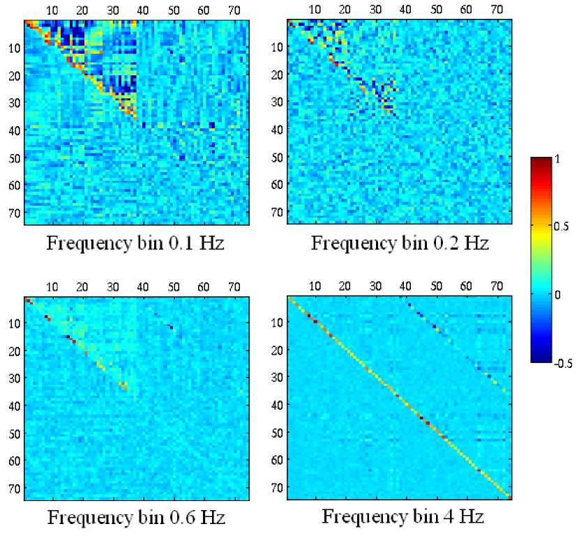
For each 1-hr constant-elevation scan set, we average the complex spectra of 100 half-scans. By comparing the average spectra over the first and the second halves (50 half-scans each) of the scan set, we checked that the noise properties are approximately stationary during a 1-hr period compared to the uncertainties in the averaged spectra. Similarly, average spectra for right-going and left-going scans were compared during a scan set to verify that there is no significant difference. To compute the noise model, we then bin the spectra into 12 logarithmically spaced frequency bands spanning 0.05–5 Hz. The average auto spectra over all PSB pairs in each frequency band are plotted in Figure 19, with the detector voltages converted to CMB temperature differences. The NETs are consistent with expectations, and are comparable to the best achieved in other ground-based experiments (Runyan et al., 2003; Hinderks et al., 2009). Before differencing, the timestreams show significant atmospheric noise below 1 Hz. This is effectively rejected by pair differencing, although there is a hint of excess low frequency noise, especially at 150 GHz. All auto and cross spectra for pair sums and pair differences are combined to form a complex noise covariance matrix at each of the 12 frequency bands, some of which are shown in Figure 20.
For the purpose of generating the noise model, the pair sum and difference timestreams are gap-filled for cosmic ray hits and electronic glitches. This procedure is not performed in making the CMB maps; any detector half-scan with a glitch is simply excluded. Because the noise covariance matrices are constructed by averaging auto and cross spectra over multiple half-scans, excluding a half-scan for a single detector pair sometimes causes the matrices to become non-positive-definite, which prevents the Cholesky decomposition necessary for the timestream simulation process described in the following section. Excluding a half-scan for all detectors if any of them contains a glitch results in data loss of up to 70% for the noise model calculation. We therefore fill gaps when possible, and reject a half-scan for all detectors if more than four PSB pairs display a simultaneous glitch.
4.2. Simulation of noise-only timestreams
For each 1-hr scan set, the measured noise covariance matrix is used in the following steps to generate simulated noise timestreams that reflect the modeled noise correlations.
(1) For each of the 12 frequency bands of the noise model spectra, we take the complex covariance matrix for sums and differences of all the good PSB pairs [7474] and compute its complex Cholesky decomposition factor [lower triangular 7474] such that .
(2) For each 20-s (200-sample) half-scan and each pair sum or difference, we generate the positive-frequency part of a complex spectrum template [74100] using normally-distributed random numbers whose magnitude has an expectation value of unity.
(3) For each of the 100 positive frequency bins of this vector of unit-spectrum templates, we multiply the Cholesky factor from the appropriate frequency band of the noise model: = . The resulting spectra have the same covariance as the data:
| (3) | |||||
(4) To ensure that these approximate the spectra of real timestreams, the negative frequency part is set to equal the complex conjugate of the positive frequency part, so that the real part is even and the imaginary part is odd.
(5) We take the inverse Fourier transform of to generate 200 samples of simulated noise time series for each of the 74 timestreams (sum and difference for the 37 PSB pairs).
To evaluate the accuracy of the noise model and simulation, the simulated timestreams were fed back into the noise modeling pipeline and the resulting power spectral distributions and covariance matrix were compared to those of the real data. The complex covariance was reproduced and the spectral amplitudes agreed to within ¡1% rms with no significant systematic differences.
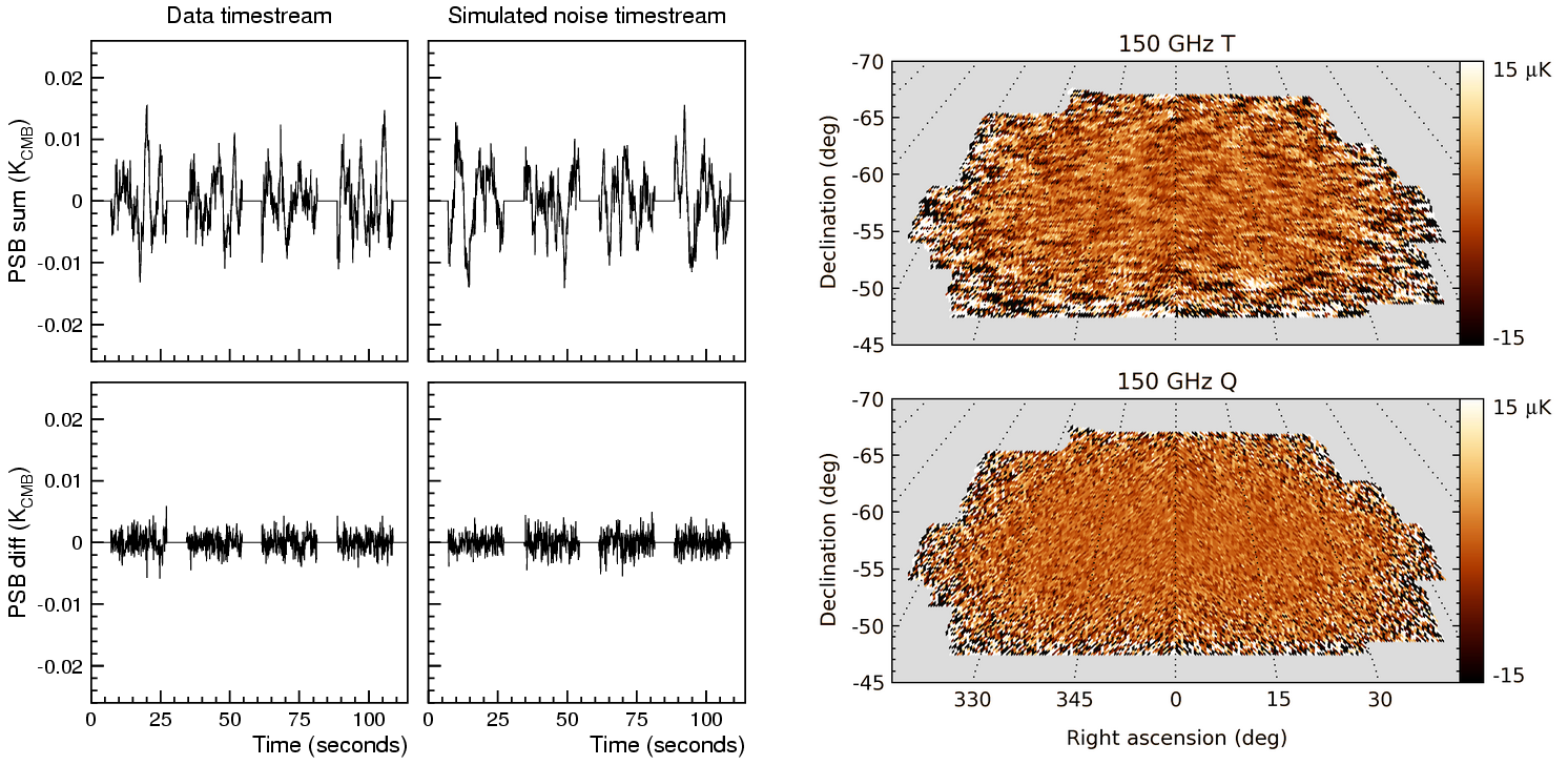
The above procedure is used to generate 500 realizations of simulated noise timestreams for the entire data set. As with the real data, scan-synchronous templates are calculated and subtracted over each set of azimuth scans, and the noise timestreams are then co-added into maps. Example noise timestreams and maps are illustrated in Figure 21.
4.3. Noise bias in power spectra
The noise bias is estimated by averaging the power spectra from an ensemble of many simulated noise-only maps (Figure 22). The noise bias in is 3 orders of magnitude smaller than the signal, and the spectrum is sample-variance limited. For the , , and cross spectra, the noise from each map is mostly uncorrelated, so the resulting are distributed around zero. However, the noise contributes a significant portion of the raw signal and is expected to dominate the power spectrum. The error bar in the final spectrum is based on the scatter in the results from an ensemble of signal+noise simulations, and for is dominated by noise.
The accuracy of the noise model can be tested by comparing the spectra of the simulated noise with those of “jackknife” maps, in which two maps made with complete halves of the data are differenced so that they are free of CMB signal and therefore nominally represent the noise level in the data. Jackknife divisions included those based on the left/right scan direction (shown in Figure 22), azimuth range, boresight rotation angle pairs, alternating observing weeks, 2006/2007 observing years, and focal plane detector split (more details in Chiang et al., 2010). We tested for evidence of noise bias amplitude misestimation using these 6 types of jackknife spectra for and at 100 and 150 GHz (a total of 24 spectra) by comparing the sum of bandpower deviations over 300–500 to those from 100 realizations of noise simulations. The set of jackknife spectra from the actual data are found to be consistent with the simulated distributions, even in this high range where the effect of noise misestimation is expected to be the largest due to the bias being a rapidly increasing function of . Repeating this test with an intentionally introduced scaling of the noise in the simulations, we find a clearly detectable departure of the sum of the actual data jackknife bandpower deviations from those of the simulated distributions. This allows us to place an upper limit on possible misestimation of the noise bias at this level, at least for a uniformly scaled error across the range.
As described above, a misestimation of noise power would correspond to a maximum shift in our estimate of 0.1 for the noise levels of the current 2-year data set. The actual 2-year constraint on , as reported in the Chiang et al. (2010) companion paper, is . The jackknife-derived upper limit on possible misestimation of the noise bias scales with the noise level. Therefore, as the noise in future data releases decreases, we can expect this internal jackknife test to continue to allow us to place upper limits on noise misestimation (or to detect it if present) at a level corresponding to roughly 1/3 of the total statistical uncertainty on , assuming a noise-limited spectrum, and less than this if a signal is detected. The final results of power spectrum estimation with noise bias removal and error bars based on simulations of signal and noise for the Bicep 2-year data are presented in the CMB results paper.
5. Conclusion
Bicep is an experiment built with a primary goal of targeting the signature of inflationary gravitational waves in the -mode polarization of the CMB at angular scales near the expected peak around 2∘. Its novel design emphasizes simplicity and systematic control, employing a carefully baffled compact cryogenic refractor and relying on a simple observing strategy of azimuth-scan modulation with periodic boresight rotation. Using Bicep’s actual data analysis pipelines, we have identified those aspects of the experiment’s instrumental and noise properties which require careful control and characterization. We have established benchmarks for these quantities corresponding to the expected -mode polarization signal for a tensor-to-scalar ratio of , a value several times smaller than the level of statistical uncertainty of the Bicep 2-year result, , or at 95% confidence (Chiang et al., 2010).
The instrumental characterization reported in this paper shows that all studied sources of potential systematic errors except for the pair relative gains, differential pointing, and possibly the noise estimation contribute to the uncertainty in the measurement at a level of . The effects which were found to be controlled to this level include differential beam size, differential ellipticity, polarization orientation uncertainty, telescope pointing, sidelobes, and thermal stability. In addition, effects which impact the overall calibration of the polarization spectra, including the absolute gain, cross-polarization response, and relative polarization orientation, have been characterized well enough to ensure that calibration uncertainty is a small fraction of our error budget.
Of the remaining three effects, the noise is estimated with sufficient accuracy to limit the uncertainty contribution to , a number that will improve as more data are added. The differential pointing of the PSB pairs is sufficiently small to meet our benchmark without correction, but will need to be taken into account to achieve lower limits on . The current uncertainty in the method we use to verify our calibration of relative detector gains in the PSB pairs leads to an upper limit in possible error on which slightly exceeds our benchmark. The uncertainty will improve as more data are included in the analysis, and a different approach may be needed if any significant relative gain errors are measured. By employing a more sophisticated analysis which allows for imperfectly-corrected differential gains of the PSB pairs and which includes the measured differential pointing, we expect to be able to control all studied sources of potential systematic errors to levels far below .
This practical experience with Bicep provides a guide for future experiments in search for the signature of inflationary gravitational waves in CMB polarization.
References
- Bock et al. (2008) Bock, J., et al. 2008, arXiv:0805.4207 [astro-ph]
- Chiang et al. (2010) Chiang, H. C., et al. 2010, Astrophys. J. , 711, 1123, arXiv:0906.1181
- Chon et al. (2004) Chon, G., Challinor, A., Prunet, S., Hivon, E., & Szapudi, I. 2004, Mon. Not. Roy. Astron. Soc. , 350, 914
- Dodelson et al. (2009) Dodelson, S., et al. 2009, arXiv:0902.3796
- Finkbeiner et al. (1999) Finkbeiner, D. P., Davis, M., & Schlegel, D. J. 1999, Astrophys. J. , 524, 867
- Górski et al. (2005) Górski, K. M., Hivon, E., Banday, A. J., Wandelt, B. D., Hansen, F. K., Reinecke, M., & Bartelmann, M. 2005, Astrophys. J. , 622, 759
- Hinderks et al. (2009) Hinderks, J. R., et al. 2009, Astrophys. J. , 692, 1221
- Hinshaw et al. (2009) Hinshaw, G., et al. 2009, Astrophys. J. Suppl. , 180, 225
- Hu et al. (2003) Hu, W., Hedman, M. M., & Zaldarriaga, M. 2003, Phys. Rev. D , 67, 043004
- Jones et al. (2003) Jones, W. C., Bhatia, R., Bock, J. J., & Lange, A. E. 2003, Proc. SPIE, 4855, 227
- Keating et al. (2003a) Keating, B. G., Ade, P. A. R., Bock, J. J., Hivon, E., Holzapfel, W. L., Lange, A. E., Nguyen, H., & Yoon, K. W. 2003a, Proc. SPIE, 4843, 284
- Keating et al. (2003b) Keating, B. G., O’Dell, C. W., Gundersen, J. O., Piccirillo, L., Stebor, N. C., & Timbie, P. T. 2003b, Astrophys. J. Suppl. , 144, 1
- Komatsu et al. (2009) Komatsu, E., et al. 2009, Astrophys. J. Suppl. , 180, 330
- Lewis et al. (2000) Lewis, A., Challinor, A., & Lasenby, A. 2000, Astrophys. J. , 538, 473
- Nolta et al. (2009) Nolta, M. R., et al. 2009, Astrophys. J. Suppl. , 180, 296
- O’Dell (2002) O’Dell, C. 2002, PhD thesis, arXiv:astro-ph/0201224
- Pryke et al. (2009) Pryke, C., et al. 2009, Astrophys. J. , 692, 1247
- Runyan et al. (2003) Runyan, M. C., et al. 2003, Astrophys. J. Suppl. , 149, 265
- Shimon et al. (2008) Shimon, M., Keating, B., Ponthieu, N., & Hivon, E. 2008, Phys. Rev. D , 77, 083003
- Yoon et al. (2006) Yoon, K. W., et al. 2006, Proc. SPIE, 6275, 62751K
- Yoon (2007) Yoon, K. W. 2007, PhD thesis, California Institute of Technology