Steady state existence of passive vector fields under the Kraichnan model

Abstract

The steady state existence problem for Kraichnan advected passive vector models is considered for isotropic and anisotropic initial values in arbitrary dimension. The models include the magnetohydrodynamic (MHD) equations, linear pressure model (LPM) and linearized Navier-Stokes (LNS) equations. In addition to reproducing the previously known results for the MHD model, we obtain the values of the Kraichnan model roughness parameter $\xi$ for which the LNS steady state exists.

I Introduction

This is a companion paper to a previous work by the present author arponen2 , wherein the phenomenon of anisotropic anomalous scaling was studied in the context of passive vector fields. The work was in part incomplete, as the main assumption was the existence of a steady state solution for the pair correlation function. We aim here to find exactly the preconditions under which this assumption is valid. Much of the technical material is from the above paper, to which we often refer for details. We study the stability of an equal time pair correlation function of a field $\mathbf{u}(t,x)$ determined by the equation

$$\dot{u}_{i}-\nu\Delta u_{i}+\mathbf{v}\cdot\nabla u_{i}-a\mathbf{u}\cdot\nabla v_{i}+\nabla_{i}P=0,$$ (1)

where the vector field $\mathbf{v}(t,x)$ is determined by the Kraichnan model kraichnan and all vector quantities are divergence free.

The model was introduced in paolo as the most general linear passive vector model respecting galilean invariance. The parameter $a=-1,0$ or $1$ corresponds respectively to the linearized Navier-Stokes equations paolo (abbreviated henceforth as LNS), the so called linear pressure modelpaolo ; arad3 ; adz ; benzi ; jurc1 ; nikolai (LPM) and the magnetohydrodynamic (MHD) equations paolo ; arad ; antonovlanottemazzino ; vergassola ; arponen ; jurc2 ; lanotte2 ; vincenzi ; kazantsev ; nikolai2 . In the context of the magnetohydrodynamic case, the inexistence of the steady state is known as the ”dynamo effect”, where the dynamo refers to exponential growth in time of the pair correlation function (see e.g. arponen ; vincenzi ; kazantsev and references therein). This problem is by far the easiest of the three due to the vanishing of the nonlocal pressure effects. In arad3 it was shown that for the linearized pressure model (corresponding to $a=0$) the steady state always exists by showing that the semi-group involved with the time evolution is always positive. The analysis for the linearized Navier-Stokes case with $a=-1$ is considerably more difficult than the above two cases since unlike in the MHD case, the nonlocal effects are present and contribute strongly to the dynamics, and because unlike in the LPM case, the semigroup is not always positive.

The present goal is therefore to find the values of $\xi$ for which the LNS steady state exists, where $\xi$ is the roughness exponent of the Kraichnan velocity field $v\sim r^{\xi}$. The method by which this is accomplished involves applying a Mellin transform on the eigenvalue equation for the two point correlation function, and by solving a resulting recursion relation.

II The model

We sketch here the derivation of the equation in Mellin transformed form and refer to the previous paper arponen2 for further details. All vector quantities in eq. (1) being divergence free results in an expression for the pressure,

$$P=(1-a)\left(-\Delta\right)^{-1}\partial_{i}v_{j}\partial_{j}u_{i}.$$ (2)

One may then rewrite the equation compactly as

$$\dot{u}_{i}-\nu\Delta u_{i}+\mathcal{D}_{ijk}\left(u_{j}v_{k}\right)=0,$$ (3)

with an integro-differential operator

$$\mathcal{D}_{ijk}=\delta_{ij}\partial_{k}-a\delta_{ik}\partial_{j}+(a-1)\partial_{i}\partial_{j}\partial_{k}\Delta^{-1},$$ (4)

where $\Delta^{-1}$ is the inverse laplacian. The equal time pair correlation is defined as

$$G_{ij}(t,\bm{r})=\langle u_{i}(t,\bm{x}+\bm{r})u_{j}(t,\bm{x})\rangle,$$ (5)

where the angular brackets denote an ensemble average with respect to the velocity field, which in turn is defined by the Kraichnan model as

$$\big{\langle}v_{i}(t,\bm{r})v_{j}(0,0)\big{\rangle} =\delta(t)D_{ij}(\bm{r})$$ (6)

$$=\delta(t)D_{1}\!\int\!\!{\mathchar 22\relax\mkern-12.0mud}^{d}\bm{q}\frac{e^{i\bm{q}\cdot\bm{r}}}{\left(\bm{q}^{2}+m_{v}^{2}\right)^{d/2+\xi/2}}P_{ij}(\bm{q})$$

where we have defined the incompressibility tensor $P_{ij}(\bm{q})=\delta_{ij}-\widehat{\bm{q}}_{i}\widehat{\bm{q}}_{j}$, ${\mathchar 22\relax\mkern-12.0mud}^{d}\bm{q}:=\frac{d^{d}q}{(2\pi)^{d}}$ and $\xi\in[0,2]$ is a parameter describing the spatial roughness of the flow.

We note a subtle difference from arponen in that we define the constant

$$D_{1}=\frac{4\xi\Gamma\left(\frac{2+d+\xi}{2}\right)}{\Gamma\left(1-\xi/2\right)}D_{0}.$$ (7)

The reason for this is that the velocity correlation and structure functions would otherwise diverge at $\xi=0$ and $\xi=2$ as the mass cutoff is removed. This aspect of the Kraichnan model has been clearly discussed in paolo.antti . The equation for the pair correlation function is then

$$\partial_{t}G_{ij}-2\nu\Delta G_{ij}-\mathcal{D}_{i\mu\nu}\mathcal{D}_{i\rho\sigma}\left(D_{\nu\sigma}G_{\mu\rho}\right)=0.$$ (8)

The Fourier transform of the correlation function will then be decomposed in terms of hyperspherical tensor basis according to the prescription in arad2 as

$$\widehat{G}_{ij}(t,\bm{p}):=\sum\limits_{a,l}B_{ij}^{a,l}(\hat{\bm{p}})\widehat{G}_{a,l}(t,p),$$ (9)

where the tensor basis components are

$$\ \left\{\begin{array}[]{ll}B_{ij}^{1,l}(\hat{\bm{p}})&=|\bm{p}|^{-l}\delta_{ij}\Phi^{l}(\bm{p})\\ B_{ij}^{2,l}(\hat{\bm{p}})&=|\bm{p}|^{2-l}\partial_{i}\partial_{j}\Phi^{l}(\bm{p})\\ B_{ij}^{3,l}(\hat{\bm{p}})&=|\bm{p}|^{-l}(p_{i}\partial_{j}+p_{j}\partial_{i})\Phi^{l}(\bm{p})\\ B_{ij}^{4,l}(\hat{\bm{p}})&=|\bm{p}|^{-l-2}p_{i}p_{j}\Phi^{l}(\bm{p})\end{array}\right.$$ (14)

and where $\Phi^{l}(\bm{p})$ is defined as $\Phi^{l}(\bm{p}):=|\bm{p}|^{l}Y^{l}(\hat{\bm{p}})$, where $Y^{l}$ is the hyperspherical harmonic function (with the multi-index $m=0$). It satisfies the properties

$$\Delta\Phi^{l}(\bm{p}) =0$$

$$\bm{p}\cdot\nabla\Phi^{l}(\bm{p}) =l\Phi^{l}(\bm{p}).$$ (15)

Note that we are concerned only with even parity and axial anisotropy. We now introduce the Mellin transform which will be used to transform the equation into a recurrence/differential equation. The method was (probably) first used in Barnes in the context of the hypergeometric function. The textbook by Hille Hille also has a useful section on the Mellin transform applied to differential equations. Appendix A of the present work also contains helpful material, and also offers some insight into some limitations of the method. We define the Mellin transform of a Fourier transform of $G$ (the anisotropy index $l$ will usually be omitted) as

$$\bar{g}_{a}(t,z)=\int\limits_{0}^{\infty}\frac{dw}{w}w^{d+z}\widehat{G}_{a}(t,w)$$ (16)

and the inversion formula

$$G_{a}(t,\bm{r})=\int_{0-}{\mathchar 22\relax\mkern-12.0mud}z|\bm{r}|^{z}\mathcal{A}_{z}\bar{g}_{a}(t,z)$$ (17)

with the definition $\mathcal{A}_{z}=\frac{\Omega_{d}}{(2\pi)^{d}}\frac{\Gamma\left(d/2\right)\Gamma\left(-z/2\right)}{2^{z+1}\Gamma\left(\frac{d+z}{2}\right)}$, which originates from the inversion of the fourier integral (with volume of the unit sphere $\Omega_{d}$), and the subscript $0-$ was used to denote a contour from $-\imath\infty$ to $+\imath\infty$ passing $z=0$ from the left (see appendix A for details). We also often denote $\bar{f}(z)\doteq\mathcal{A}_{z}\bar{g}(z)$, which is just the ordinary Mellin transform.

Applying the Fourier transform, dividing by $p^{2}$, applying the Mellin transform and finally setting the cutoff parameter $m_{v}$ to zero in eq. (1) (see arponen2 for details), we obtain the complex recurrence/differential equation

$$\partial_{t}\bar{g}_{a}(t,z-2)+2\nu\bar{g}_{a}(t,z)-\widetilde{\lambda}\bar{g}_{a}(t,z-\xi)-\mathrm{T}^{ab}_{d+\xi,d+z-\xi}\bar{g}_{b}(t,z-\xi)=0,$$ (18)

with the definitions

$$\widetilde{\lambda}=(a-1)\left(d+1+a(1-\xi)\right)\frac{d\pi\xi\Gamma(d/2)c_{d}}{16\sin(\pi\xi/2)\Gamma\left(\frac{d-\xi}{2}+2\right)\Gamma\left(\frac{d+\xi}{2}+1\right)}$$ (19)

and

$$\mathrm{T}^{ab}_{2\alpha,2\beta}=\frac{4\xi\Gamma\left(\frac{d+\xi}{2}\right)}{\Gamma\left(1-\xi/2\right)}\frac{\Gamma(d/2+l-\alpha)\Gamma(d/2-\beta)\Gamma(\alpha+\beta-d/2)}{\Gamma(\alpha)\Gamma(\beta)\Gamma(d+l-\alpha-\beta)}\tau^{ab}(z),$$ (20)

where the matrix coefficients $\tau^{ab}(z)$ are listed in the appendix of arponen2 . We have also effectively set $D_{0}=1$ by redefining time and viscosity. Requiring the correlation function (9) to be divergence free, i.e. zero when contracted with $p_{i}$, results in only two of the four coefficients $\bar{g}_{a}$ being independent. The resulting equation may then be written in the following form,

$$\partial_{t}\mathbf{\bar{h}}(t,z+\xi-2)+2\nu\mathbf{\bar{h}}(t,z+\xi)-\left(\widetilde{\lambda}\mathbf{1}+\mathbf{A}+\mathbf{B}\cdot\mathbf{X}\right)\mathbf{\bar{h}}(t,z)=0.$$ (21)

Here we have performed a translation $z\to z+\xi$, defined the vector quantity $\mathbf{\bar{h}}=\left(\bar{g}_{1},\bar{g}_{2}\right)^{\mathrm{T}}$ and the matrices by

$$\mathbf{T}_{d+\xi,d+z}=\begin{pmatrix}\mathbf{A}&\mathbf{B}\\ \mathbf{C}&\mathbf{D}\end{pmatrix}\ \ \ ,\ \ \ \mathbf{X}=\begin{pmatrix}0&-(l-1)\\ -1&l(l-1)\end{pmatrix}.$$ (22)

II.1 Isotropic sector

We will be mostly concerned with the isotropic case since much of the actual computations can be neatly performed all the way. For $l=0$, only the tensors $B^{1}$ and $B^{4}$ are nonzero, and correspondingly in the tensor decomposition we only have the coefficients $\bar{g}_{1}(z)$ and $\bar{g}_{4}(z)=-\bar{g}_{1}(z)$ (due to the divergence free condition). The equation (21) then becomes a scalar equation for $\bar{g}_{1}(z)$ alone, hence we only need the $(1,1)$ component of the matrix $\left(\widetilde{\lambda}\mathbf{1}+\mathbf{A}+\mathbf{B}\cdot\mathbf{X}\right)$, which reads explicitly

$$\left(\widetilde{\lambda}\mathbf{1}+\mathbf{A}+\mathbf{B}\cdot\mathbf{X}\right)_{11}=\frac{2(a-1)(a\xi-1-a-d)\Gamma\left(1+\xi/2\right)\Gamma\left(1+d/2\right)}{\Gamma\left(\frac{4+d-\xi}{2}\right)}$$

$$-p_{a}(z)\frac{\Gamma\left(-z/2\right)\Gamma\left(\frac{d+z+\xi}{2}\right)}{2\Gamma\left(\frac{2+d+z}{2}\right)\Gamma\left(\frac{4-z-\xi}{2}\right)}\doteq\Lambda^{a}_{\xi}(z),$$ (23)

where

$$p_{a}(z)=-(a-1)^{2}(d+1)\xi(2-\xi)$$

$$+(z+\xi-2)\left((d-1)z^{2}+\left(d(d-1)+2a\xi\right)z+\right.$$

$$\left.\xi\left(-d-1+2a(d+1)-a^{2}(1+2d-d^{2}+\xi-d\xi)\right)\right)$$ (24)

The equation in the isotropic sector is then

$$\partial_{t}\bar{g}_{1}(t,z+\xi-2)+2\nu\bar{g}_{1}(t,z+\xi)-\Lambda^{a}_{\xi}(z)\bar{g}_{1}(t,z)=0.$$ (25)

III The method

We now consider the eigenvalue problem with $\bar{g}_{1}(t,z)\propto e^{-Et}g(z)$, resulting in the equation

$$E\bar{g}(z+\xi-2)-2\nu\bar{g}(z+\xi)+\Lambda^{a}_{\xi}(z)\bar{g}(z)=0.$$ (26)

This is analogous to the Schrödinger method in vergassola ; vincenzi ; kazantsev . The steady state exists if one can show that the spectrum is nonnegative. However, for example in the magnetohydrodynamic case as in the above mentioned papers and in arponen , it was shown that there exists a critical value of the parameter $\xi$ above which one has negative energies resulting in an exponential growth in time. This phenomenon is interpreted as the dynamo effect of magnetic fields. Previous studies on the dynamo problem have resorted to some approximative or numerical schemes to find the growth rate $|E|$ as a function of $\xi$. Here we will settle for simply finding the values of $\xi$ for which the energies are nonnegative, thus implying a steady state. This is done by studying the zero energy equation, i.e. setting $E=0$. This has the advantage of providing us with an exact solution, up to a numerical solution of a transcendental equation.

The argument used in the present work is closely analogous to the classic ”node theorem” (see e.g. reedsimon and also appendix A), which can be roughly stated as follows. Suppose that for some large enough value of $E$ the corresponding solution $f_{E}(r)$ is oscillating between positive and negative values ar large $r$ and satisfies the boundary condition $f_{E}(L)=0$, for some large $L$ (tending to infinity). If the spectrum is bounded from below, we know that by decreasing $E$ the zeros of $f_{L}(r)$ will move to the right and satisfy the boundary condition for a discrete set of $E$. The value of $E$ for which the smallest zero reaches $L$ is then the ground state energy. Since we are interested in whether or not the ground state is positive or negative, we can instead study the zero energy equation and ask for which values of $\xi$ the solution crosses over from nonoscillating to oscillating. We know that the $\xi=0$ equation corresponds to diffusion, i.e. a nonoscillating zero energy ground state. As we increase $\xi$, we may discover that the solution becomes oscillating at large scales, which would imply a negative energy ground state and therefore instability. The large scale behavior of the solutions is determined by the negative poles of the Mellin transform, so the problem is then reduced to finding these poles and determining if and when they become complex valued.

IV Isotropic sector of LNS

The stability problem in the linearized Navier-Stokes case is closely related to the laminar flow stability problem as described in §26 of landau . The equation is derived from the Navier-Stokes equation by decomposing the velocity field into $\mathbf{v}(\bm{r})+\mathbf{u}(t,\bm{r})$, where $\mathbf{v}$ is a stationary solution and $\mathbf{u}$ is a small perturbation, resulting in the equation

$$\dot{u}_{i}-\nu\Delta u_{i}+\mathbf{v}\cdot\nabla u_{i}+\mathbf{u}\cdot\nabla v_{i}+\nabla_{i}P=0.$$ (27)

The question is then whether or not the laminar flow is stable under such perturbations. Here instead the field $\mathbf{v}$ is supposed to model a statistical steady state solution of the full Navier-Stokes turbulence, as prescribed by the Kraichnan model. We are therefore studying whether or not the Kraichnan model is an adequate steady state description of turbulence in terms of stability. For $a=-1$ we now have

$$\Lambda^{-}_{\xi}(z)=\frac{4(d+\xi)\Gamma\left(1+\xi/2\right)\Gamma\left(1+d/2\right)}{\Gamma\left(\frac{4+d-\xi}{2}\right)}-p_{-1}(z)\frac{\Gamma\left(-z/2\right)\Gamma\left(\frac{z+d+\xi}{2}\right)}{2\Gamma\left(\frac{z+d+2}{2}\right)\Gamma\left(\frac{4-\xi-z}{2}\right)},$$ (28)

where

$$p_{-1}(z) =(z+\xi)\left(-2z+2\xi+d^{2}(z+\xi-2)\right.$$ (29)

$$\left.-(z+\xi)^{2}+d(2+(z-3)z-(3-\xi)\xi)\right)+4z^{2}.$$

The problem is obviously a more difficult one than in the MHD case due to the transcendental nature of the function $\Lambda_{\xi}^{-}$. We can however expand it as an infinite product of zeros and poles according to the Weierstrass factorization theorem (see e.g. conway ). The function $\Lambda_{\xi}^{-}$ may then be rewritten as

$$\Lambda_{\xi}^{-}(z)=e^{s(z)}\prod\limits_{k=1}^{\infty}\frac{\left(z-a_{k}^{+}\right)\left(z-a_{k}^{-}\right)}{\left(z-b_{k}^{+}\right)\left(z-b_{k}^{-}\right)}e^{\delta/k},$$ (30)

where the $+$ and $-$ signs refer to zeros or poles that have respectively positive (or zero) or negative real parts, see Fig. (2). We also have the poles $b_{k}^{+}=2k$, $b_{k}^{-}=-d-\xi-2k$ and $s(z)$ is some unknown entire function on the complex plane and $\delta$ is a $z$ -independent Weierstrass factor that enforces convergence of the infinite product. It can be derived by showing that asymptotically as $z\to\pm\infty$, the poles and zeros of eq. (28) behave respectively as $\pm 2k+\text{const.}$ where the constant term depends on $\xi$ and $d$. It may certainly be possible to derive bounds for $s(z)$ by asymptotic analysis of eq. (28), but since it can not contribute to the pole or zero structure of the solution, we refrain from doing so. We can also neglect the explicit form of the constant $\delta$ for the same reason. The zero energy equation from (26), rewritten here as

$$\bar{g}(z) =\frac{2\nu}{\Lambda_{\xi}^{-}(z)}\bar{g}(z+\xi),$$ (31)

can then be solved by the same methods as in appendix A with the strip of analyticity requirement $-\xi<\mathcal{R}e(z)<0$, resulting in

$$\bar{g}(z) =\sigma_{\xi}(z)\Psi(z)(2\nu)^{-z/\xi}$$ (32)

$$\times\prod\limits_{k>0}e^{z\delta/\xi k}\frac{\Gamma\left(\frac{z-a_{k}^{-}}{\xi}\right)\Gamma\left(\frac{2k+\xi-2-z}{\xi}\right)}{\Gamma\left(\frac{a_{k}^{+}+\xi-z}{\xi}\right)\Gamma\left(\frac{2k+z+d+\xi-2}{\xi}\right)}$$

where $\Psi(z)$ satisfies the equation $\Psi(z)=e^{-s(z)}\Psi(z+\xi)$, whose solution is again an exponential of an entire function. The following subtlety concerning the above formula should be observed: we deliberately chose to use the form $\sim 1/\Gamma(1-x)$ instead of $\Gamma(x)$, where the two are related by the Euler reflection formula $\Gamma(-z/2)\Gamma(1+z/2)=-\pi/\sin(\pi z/2)$. The reason is that only in this form the strip of analyticity remains pole free, as per the consistency requirement. For example using $\Gamma\left(\frac{z-a_{k}^{+}}{\xi}\right)$ in the above result would introduce poles at $z=a_{k}^{+}-\xi n$ for positive integers $n$, that would eventually permeate the strip of analyticity. However, in some cases as we increase $\xi$, the poles will enter the strip of analyticity and render the solution incompatible with the strip of analyticity requirement. We will also demand that the solution converges to zero at imaginary infinities in order to justify the shift of integration contour (see appendix A). It seems quite difficult to deduce the asymptotic behavior from the above formula, but we can study it by an asymptotic expansion of the exact form of eq. (28). The function $\Lambda_{\xi}^{-}(z)$ behaves asymptotically as $\sim z^{\xi}$ at imaginary infinities, so the asymptotic version of the difference equation (31) reads

$$\bar{g}(z)=z^{-\xi}\bar{g}(z+\xi)$$ (33)

up to some irrelevant constant term. The asymptotic solution is then $\bar{g}(z)=\sigma_{\xi}(z)\Gamma(z)^{\xi}$. Multiplication by $\Gamma(-z/2)/\Gamma\left((z+d)/2\right)$ in defining $\bar{f}$ introduces a pole at $z=0$, which takes care of the boundary condition. Then we have asymptotically $\bar{f}(z)\sim\sigma_{\xi}(z)e^{-\frac{\pi}{\xi}y}y^{(\xi-1)(x-1/2)}$, where $z=x+\imath y$. Fourier expansion of $\sigma_{\xi}$ would then contain terms such as $\sin\left(\frac{2\pi}{\xi}nz\right)$, which would spoil integrability for $0<\xi<2$, unless $n=0$. Therefore $\sigma_{\xi}(z)$ has to be a constant.

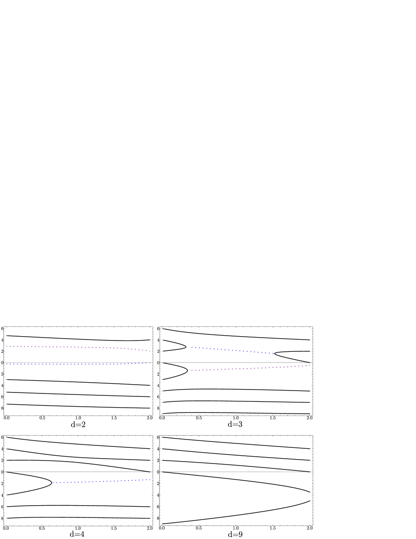
Figure 1: A plot of the $a=-1$ poles of the solution $\bar{g}(z)$ in the isotropic sector versus $\xi$ in various dimensions. The dashed curves denote the real parts of complex valued poles. There is an infinity of poles, but all the others not displayed here are real. Also, all the poles in dimensions $d\geq 9$ are real in $0\leq\xi\leq 2$.

We see now that the poles of $\bar{f}(z)$ occur for non-negative integers $n$ at $z=\xi-2+2k+\xi n$, $z=2(k-1)$ (with $k>0$) and at $z=a_{k}^{-}-\xi n$, where only the latter affects the large scale behavior. We draw the important conclusion that the poles $a_{k}^{+}$ have no effect on the steady state existence problem. By looking at Fig. (1) we can see how the first few large scale poles $a_{k}^{-}$ behave in various dimensions. In two dimensions the leading pole $a_{1}^{-}$ enters the strip at around $\xi\approx 0.28$ and is complex for all $\xi$, which implies that there is no steady state at all in the isotropic sector, at least for $\xi<0.28$ . In three dimensions the poles $a_{1}^{-}$ and $a_{2}^{-}$ become complex at around $\xi_{c}\approx 0.345$ and enter the strip of analyticity at around $\xi\approx 1.08$. Similar behavior occurs with different $\xi_{c}$ in higher dimensions, until at $d=9$ the poles stay real for all $0\leq\xi\leq 2$. We have plotted the value of $\xi_{c}$ in Fig. (2) in dimensions $2\ldots 9$ together with the magnetohydrodynamic case. The fact that in some cases for large enough $\xi$ the strip of analyticity condition is violated could possibly mean that the steady state exists also for some large values of $\xi$. We will however be content with studying the cases for which such a violation does not take place.

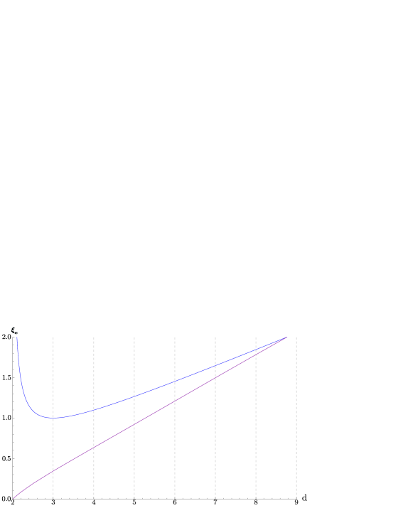
Figure 2: A plot of the critical value $\xi_{c}$, above which the flow becomes unstable, versus the space dimension $d$. The upper curve refers to the magnetohydrodynamic case with $a=1$ and the lower to the linearized Navier-Stokes case with $a=-1$.

One important lesson of the present section is that the ”complexification” hypothesis of arponen2 ; arponen is indeed an indication of instability of the flow, in the sense that the imaginary parts of the scaling exponents correspond to oscillations of the correlation function and are therefore responsible for the instability. The second lesson is that one only needs to be concerned with the negative zeros $a_{k}^{-}$ of $\Lambda_{\xi}^{a}(z)$ when considering the stability problem, since they become the poles in the solution $\bar{f}(z)$. The positive zeros $a_{k}^{+}$ appear only as zeros in $\bar{f}(z)$.

V Anisotropic sectors of LNS

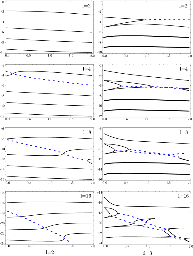
Figure 3: A figure showing the leading large scale poles $a_{k}^{-}$ in various anisotropic sectors in two and three dimensions. The dashed lines denote the real parts of complex valued poles. The thick curves denote two poles very close to each other. All the poles beyond what are shown here are real for $0<\xi<2$.

The anisotropic sectors can be studied with the same methods as above. We will however refrain from performing the actual computations and simply extend what we have learned from the isotropic sector to the anisotropic case, namely that one simply needs to study the complexification of the negative poles of the solution $\bar{f}_{a}(z)$ (we now have a matrix equation). The role of $\Lambda_{\xi}$ will now be taken by the determinant of the matrix in eq. (21), instead of just the $(1,1)$ component. Since we already know that the flow is stable in the anisotropic sectors for $a=1$ and $a=0$ (see e.g. arad2 ; arad3 ), we concentrate only on the $a=-1$ case in various dimensions. The anisotropic linearized Navier-Stokes exponents differ from the magnetohydrodynamic ones in that even if the leading exponent is real, the next to leading exponent may be complex valued, resulting in oscillating behavior at intermediate scales. These exponents however have no effect on the existence problem. This is because the boundary condition at $R$ tending to infinity can only be satisfied by the leading oscillating exponent. We also need to make sure that the periodic function $\sigma_{\xi}(z)$ is again required to be a constant due to integrability, so that it will not cancel with any of the poles. This results from the fact that all matrix coefficients beside the (1,1) coefficient in eq. (23) behave asymptotically as $\sim z^{\xi}$ irrespectively of $l$ , and therefore so does the determinant. Hence the same conclusions will be drawn as in the isotropic case, i.e. that $\sigma_{\xi}$ is indeed a constant.

We have plotted some leading negative exponents in various anisotropic sectors in two and three dimensions in fig. (3). In two dimensions the leading anisotropic exponent is real, except (strangely enough) for $\xi\lesssim 0.15$. The anisotropic sectors are therefore quite stable in comparison to the completely unstable isotropic sector. In three dimensions the $l=2$ anisotropic leading exponent becomes complex at $\xi_{c}^{(2)}\approx 0.937$ and all the higher sectors have purely real leading exponents. The anisotropic sectors are therefore much more stable in comparison to the isotropic sector critical value $\xi_{c}^{(0)}\approx 0.345$, somewhat similarly to the magnetohydrodynamic case. We also note that none of the poles lie inside the strip of analyticity, so the results should hold for all $\xi$. In dimensions $d\geq 4$ the anisotropic exponents are always real.

VI Conclusion

The stability analysis of the passive vector models previously considered in a companion paper arponen2 was successfully completed. The critical value $\xi_{c}$ below which the steady state exists was found in all dimensions, although the possibility of a steady state for an even larger region could not be excluded in the isotropic sector. The reason for flow instability was shown to be caused by the complexification of the largest negative pole of the solution, corresponding to large scale behavior of the correlation function. It was observed that in two dimensions the linearized Navier-Stokes problem is not stable for any $\xi>0$ in the isotropic sector, but relatively stable in the anisotropic sectors. In three dimensions the isotropic sector was observed to be stable for $\xi\lesssim 0.345$, the $l=2$ anisotropic sector for $\xi\lesssim 0.937$ and higher anisotropic sectors for all $\xi$. In dimensions from four to eight, the isotropic sector is stable below the critical values plotted in Fig. (2) and the anisotropic sectors are stable for all $\xi$. In dimensions $d\geq 9$, all sectors are stable for all $\xi$.

Appendix A Mellin transform and examples

The Mellin transform has been used to solve differential equations previously in e.g. Hille ; Barnes . The purpose of the present appendix is to clarify some aspects of the Mellin transform method and to point out some of its limitations.

A.1 Solving differential equations by Mellin transform

Define the Mellin transform of a function $f(r)$ with $r\geq 0$ as

$$\bar{f}(z)\doteq\int\limits_{0}^{\infty}\frac{dw}{w}w^{-z}f(w).$$ (34)

We will be concerned with finite diffusivity/viscosity $\nu$ in our equations, which amounts to $f(0)\doteq 1$ (neglecting normalization), and power law or faster decay at infinity with some so far unknown exponent $-\zeta$. The complex parameter $z$ in the above formula is therefore restricted to $-\mathcal{R}e(\zeta)<\mathcal{R}e(z)<0$ . The inverse transform is then

$$f(r)\doteq\int\limits_{c-\imath\infty}^{c+\imath\infty}\!\!{\mathchar 22\relax\mkern-12.0mud}z\bar{f}(z)r^{z}$$ (35)

where $-\mathcal{R}e(\zeta)<c<0$. Because of the constant boundary condition at zero, $\bar{f}(z)$ must have a pole at $z=0$. We will therefore take $c=0$ such that the contour will pass $z=0$ from the left, and denote this by $0-$ under the integration sign. We can now use the Mellin transform to define a differential/integral operator of order $\sigma$ as

$$(\widehat{D}_{\sigma}f)(r)\doteq\int_{0-}\!\!{\mathchar 22\relax\mkern-12.0mud}z\Delta_{\sigma}(z)\bar{f}(z)r^{z-\sigma}.$$ (36)

For example the derivative $\partial_{r}$ would correspond to $\sigma=1$ and $\Delta_{1}(z)=z$. Consider now the equation

$$(\widehat{D}_{\sigma}f)(r)+\lambda f(r)=0$$ (37)

with the above mentioned boundary conditions. Expressing this with the help of the Mellin transforms yields

$$\int_{0-}\!\!{\mathchar 22\relax\mkern-12.0mud}z\Delta_{\sigma}(z)\bar{f}(z)r^{z-\sigma}+\lambda\int_{0-}\!\!{\mathchar 22\relax\mkern-12.0mud}z\bar{f}(z)r^{z}$$

$$=\int_{0-}\!\!{\mathchar 22\relax\mkern-12.0mud}z\Delta_{\sigma}(z)\bar{f}(z)r^{z-\sigma}+\lambda\int_{\sigma-}\!\!{\mathchar 22\relax\mkern-12.0mud}z\bar{f}(z-\sigma)r^{z-\sigma}$$

$$=\int_{0-}\!\!{\mathchar 22\relax\mkern-12.0mud}z\left\{\Delta_{\sigma}(z)\bar{f}(z)+\lambda\bar{f}(z-\sigma)\right\}r^{z-\sigma}+\sum_{i}r^{z_{i}}\mathcal{R}(\bar{f}(z_{i}))\equiv 0,$$ (38)

where in the second term on the second line we have simply changed the integration variable $z\to z-\sigma$ and shifted the contour from $\sigma\to 0$ on the third line (assuming sufficiently fast decay at imaginary infinities), and also denoted in the last sum the possible contribution of poles inside the strip $-\sigma<z<0$. We can solve the problem by solving the recursion equation

$$\Delta_{\sigma}(z)\bar{f}(z)+\lambda\bar{f}(z-\sigma)=0$$ (39)

but only if we can find a solution for which the strip of analyticity is pole free, i.e. that the sum of residues above vanishes, which also implies $\mathcal{R}e(\zeta)>\sigma$. It turns out that in the present context there are situations where such solutions cannot be found, at least not without improving the present procedure. We will however be able to find a sufficiently large class of solutions for which this problem does not appear.

A.2 Isotropic $a$ -model equation for $\xi=2$

For $\xi=2$ the problem becomes simple enough to be solved exactly even for nonzero energies. From eq. (23) we have now

$$\Lambda^{a}_{2}(z)=(d-1)z^{2}+\left(4a+d(d-1)\right)z+2a\left(d+a(d^{2}-2)\right)$$ (40)

and the equation (26) can now be written as

$$\left(z-z_{+}\right)\left(z-z_{-}\right)\bar{g}(z)=2\nu\bar{g}(z+2),$$ (41)

where we have defined the roots

$$z_{\pm}=\frac{-4a-d(d-1)\pm\sqrt{D_{E}}}{2(d-1)}$$ (42)

with the discriminant

$$D_{E}=-4(d-1)E+d^{2}+d(d-2)\left(d^{2}-8(d+1)a^{2}\right).$$ (43)

Employing the definition $\bar{f}(z)\doteq\mathcal{A}_{z}\bar{g}(z)\propto\frac{\Gamma\left(-z/2\right)}{2^{z}\Gamma\left(\frac{z+d}{2}\right)}\bar{g}(z)$ and a translation $z\to z-2$, we obtain the equation

$$\frac{z(z+d-)}{(z-z_{+}-2)(z-z_{-}-2)}\bar{f}(z)+\frac{1}{2\nu}\bar{f}(z-2)=0,$$ (44)

which should be compared to eq. (39). A general solution to eq. (44) can be written as

$$\bar{f}(z)=(2\nu)^{-z/2}\frac{\sigma_{2}(z)}{\sin\left(\pi z/2\right)}\frac{\Gamma\left(\frac{z-z_{+}}{2}\right)\Gamma\left(\frac{z-z_{-}}{2}\right)}{\Gamma\left(\frac{z+2}{2}\right)\Gamma\left(\frac{z+d}{2}\right)}$$ (45)

where $\sigma_{2}(z+2)=\sigma_{2}(z)$ is a so far arbitrary periodic function (with the subscript denoting the period). The solution (modulo the $\sigma_{2}$ -term) has poles at $z=2n$ and $z=z_{\pm}-2n$ for nonnegative integer $n$. The width of the strip of analyticity therefore has to be $-2<\mathcal{R}e(z)<0$, from which we conclude that $\sigma_{2}(z)$ must be an entire, periodic function and that the poles $\mathcal{R}e(z_{\pm})<-2$. At imaginary infinities the above solution behaves asymptotically as

$$\bar{f}(z)\sim(2\nu)^{-z/2}\sigma_{2}(z)e^{-\frac{\pi}{2}|z|}z^{a-1}.$$ (46)

Since $\sigma_{2}(z)$ is entire, we can expand it in Fourier series as $\sigma_{2}(z)=\sum\limits_{k\geq 0}a_{k}\sin\left(k\pi z\right)$. Anything else than $k=0$ would however spoil the above asymptotic behavior, so we conclude that $\sigma_{2}(z)=\text{const}$. Inverting the Mellin transform then yields

$$G(r)=C_{1}\int_{0-}\!\!{\mathchar 22\relax\mkern-12.0mud}z\frac{\Gamma\left(\frac{z-z_{+}}{2}\right)\Gamma\left(\frac{z-z_{-}}{2}\right)}{\Gamma\left(\frac{z+2}{2}\right)\Gamma\left(\frac{z+d}{2}\right)}\frac{\left(r^{2}/2\nu\right)^{z/2}}{\sin\left(\pi z/2\right)},$$ (47)

which is what one would obtain e.g. in the MHD problem with $a=1$ by a direct coordinate space solution arponen . The MHD problem for $\xi\neq 2$ can also be easily solved, although we will not reproduce that calculation here. The ground state energy is then the value of $E$ for which the discriminant $D_{E}$ vanishes (crossover between oscillating and power law decay), i.e.

$$E_{0}=\frac{d\left(d^{3}-10d^{2}+9d+16\right)}{4(d-1)},$$ (48)

which is negative for $3\leq d\leq 8$ implying a dynamo effect for $\xi=2$. It is now tempting to use the above solution also for other values of $a$. However, for example for $a=-1$ and $d=3$ we have

$$z_{\pm}=-\frac{1}{2}\pm\frac{1}{2}\sqrt{-2E-15}$$ (49)

which means that for energies $E\geq-15/2$, the poles $z_{\pm}$ are always inside the strip of analyticity. We must therefore conclude that in cases such as this, the method is not sufficient to determine the existence of a steady state.

References

- (1) H. Arponen. Anomalous scaling and anisotropy in models of passively advected vector fields. Phys. Rev. E, 79(5):056303, May 2009.
- (2) Robert H. Kraichnan. Anomalous scaling of a randomly advected passive scalar. Phys. Rev. Lett., 72(7):1016–1019, Feb 1994.
- (3) L. Ts. Adzhemyan, N. V. Antonov, A. Mazzino, P. Muratore-Ginanneschi, and A. V. Runov. Pressure and intermittency in passive vector turbulence. EPL (Europhysics Letters), 55(6):801–806, 2001.
- (4) Itai Arad and Itamar Procaccia. Spectrum of anisotropic exponents in hydrodynamic systems with pressure. Phys. Rev. E, 63(5):056302, Apr 2001.
- (5) L. Ts. Adzhemyan, N. V. Antonov, and A. V. Runov. Anomalous scaling, nonlocality, and anisotropy in a model of the passively advected vector field. Phys. Rev. E, 64(4):046310, Sep 2001.
- (6) R. Benzi, L. Biferale, and F. Toschi. Universality in passively advected hydrodynamic fields: the case of a passive vector with pressure. The European Physical Journal B, 24:125, 2001.
- (7) N. V. Antonov, Michal Hnatich, Juha Honkonen, and Marian Jurčišin. Turbulence with pressure: Anomalous scaling of a passive vector field. Phys. Rev. E, 68(4):046306, Oct 2003.
- (8) L. Ts. Adzhemyan, N. V. Antonov, and A. V. Runov. Anomalous scaling, nonlocality, and anisotropy in a model of the passively advected vector field. Phys. Rev. E, 64(4):046310, Sep 2001.
- (9) H. Arponen and P. Horvai. Dynamo effect in the kraichnan magnetohydrodynamic turbulence. J. Stat. Phys., 129(2):205–239, Oct 2007.
- (10) A. P. Kazantsev. Enhancement of a magnetic field by a conducting fluid flow. Sov. Phys. JETP, 26:1031, 1968.
- (11) D. Vincenzi. The Kraichnan-Kazantsev dynamo. J. Stat. Phys., 106(5–6):1073–1091, March 2002.
- (12) M. Vergassola. Anomalous scaling for passively advected magnetic fields. Phys. Rev. E, 53(4):R3021–R3024, Apr 1996.
- (13) I. Arad, L. Biferale, and I. Procaccia. Nonperturbative spectrum of anomalous scaling exponents in the anisotropic sectors of passively advected magnetic fields. Phys. Rev. E, 61(3):2654–2662, Mar 2000.
- (14) N. V. Antonov, A. Lanotte, and A. Mazzino. Persistence of small-scale anisotropies and anomalous scaling in a model of magnetohydrodynamics turbulence. Phys. Rev. E, 61(6):6586–6605, Jun 2000.
- (15) M. Hnatich, J. Honkonen, M. Jurcisin, A. Mazzino, and S. Sprinc. Anomalous scaling of passively advected magnetic field in the presence of strong anisotropy. Physical Review E (Statistical, Nonlinear, and Soft Matter Physics), 71(6):066312, 2005.
- (16) A. Lanotte and A. Mazzino. Anisotropic nonperturbative zero modes for passively advected magnetic fields. Phys. Rev. E, 60(4):R3483–R3486, Oct 1999.
- (17) N. V. Antonov, A. Lanotte, and A. Mazzino. Persistence of small-scale anisotropies and anomalous scaling in a model of magnetohydrodynamics turbulence. Phys. Rev. E, 61(6):6586–6605, Jun 2000.
- (18) Itai Arad, Victor S. L’vov, and Itamar Procaccia. Correlation functions in isotropic and anisotropic turbulence: The role of the symmetry group. Phys. Rev. E, 59(6):6753–6765, Jun 1999.
- (19) E. W. Barnes. A New Development of the Theory of the Hypergeometric Functions. Proc. London Math. Soc., s2-6(1):141–177, 1908.
- (20) E. Hille. Ordinary differential equations in the complex domain. John Wiley & Sons Inc., 1976.
- (21) M. Reed and B. Simon. Methods of modern mathematical physics IV: Analysis of operators. Academic press, 1978.
- (22) L. D. Landau. Fluid Mechanics, 2nd. edition, Volume 6. Elsevier, 1987.
- (23) J.B. Conway. Functions of one complex variable I. Springer, 1978.
- (24) http://mathstat.helsinki.fi/mathphys/paolo_files/zero-modes.php
- (25) P. Muratore-Ginanneschi and A. Kupiainen. Scaling, Renormalization and Statistical Conservation Laws in the Kraichnan Model of Turbulent Advection. J. Stat. Phys., 126(3):669–724, Feb 2007.