The Clowes-Campusano Large Quasar Group Survey: I. GALEX selected sample of LBGs at z$\sim$1.

Abstract

The nature of galaxy structures on large scales is a key observational prediction for current models of galaxy formation. The SDSS and 2dF galaxy surveys have revealed a number of structures on 40-150 h^-1 Mpc scales at low redshifts, and some even larger ones. To constrain galaxy number densities, luminosities, and stellar populations in large structures at higher redshift, we have investigated two sheet-like structures of galaxies at $z$=0.8 and 1.3 spanning 150 h^-1 comoving Mpc embedded in large quasar groups extending over at least 200 h^-1 Mpc. We present first results of an analysis of these sheet–like structures using two contiguous 1 deg GALEX fields (FUV and NUV) cross-correlated with optical data from the Sloan Digital Sky Survey (SDSS). We derive a sample of 462 Lyman Break Galaxy (LBG) candidates coincident with the sheets. Using the GALEX and SDSS data, we show that the overall average spectral energy distribution of a LBG galaxy at $z\sim$1 is flat (in f_λ) in the rest frame wavelength range from 1500Å  to 4000Å, implying evolved populations of stars in the LBGs. From the luminosity functions we get indications for overdensities in the two LQGs compared to their foreground regions. Similar conclusions come from the calculation of the 2-point correlation function, showing a 2$\sigma$ overdensity for the LBGs in the $z\sim 0.8$ LQG on scales of 1.6 to 4.8 Mpc, indicating similar correlation scales for our LBG sample as their $z\sim 3$ counterparts.

1 Introduction

The relation between galaxy populations, environment, and the quasar/AGN phase of galaxy evolution is crucial for a complete picture of galaxy and structure formation. Galaxy redshift surveys have revealed the cosmic web, a cellular distribution (e.g. Doroshkevich & Dubrovich, 2001) on scales of 40-150 h^-1 Mpc or more. In particular, large structures were found in the SDSS and 2dF redshift survey (Adelman-McCarthy et al., 2006; Croom et al., 2004), tracing galaxy populations and star formation in the cosmic web. The $\Lambda$CDM model predicts weakly non-linear structures of these dimensions at low redshift, but simulations (e.g. Evrard et al., 2002) indicate that “Great Wall”-like sheets become rare at $z\sim$1. Clearly the detection of very large filaments and the presence of a large number of high redshift clusters are an interesting test of current cosmologies. Distinct blue and red galaxy sequences at $0<z<0.7$ indicate significant environmental effects on the red fraction at fixed luminosity (e.g. Balogh et al., 2004; Cassata et al., 2007). Environmental effects are especially key in triggering/quenching star formation through mergers, harassment, and gas stripping (Postman et al., 2005), though on cluster outskirts, some star formation also goes on (Duc et al., 2002; Coia et al., 2005). There is clear evidence that galaxies in filaments falling into clusters of galaxies undergo bursts of star formation prior to reaching the cluster, both at low redshifts (Porter et al., 2008) and at $z\sim 1$ (Koyama et al., 2008) even though the specific star formation rates may be lower for those galaxies in the red sequence (e.g., Nakata et al., 2002). Understanding these mechanisms is essential to assess the role of environment in galaxy evolution.

Extremely dense regions should show the most extreme environmental effects. The epoch $z\sim 1$ is a key point, where the galaxy luminosity function (LF) still can be readily probed to faint levels and environmental effects appear to affect galaxy evolution strongly. Recent work (Gerke et al., 2007; Noeske et al., 2007) indicates that $z\sim 1-1.5$ is where the galaxy color-density relation establishes itself: at lower $z$ red galaxies prefer dense environments, while at earlier times star-forming and passive galaxies inhabit similar environments, with possible evidence for an inversion (Cooper et al., 2007, 2008; Elbaz et al., 2007). However, Quadri et al. (2007) find that the color-density relation (in the sense of redder galaxies being located in denser environments) extends to redshifts $z>2$. Hence studies of galaxies in overdense environments at this epoch promise to yield crucial insights into this critical part of galaxy formation theory.

Quasars may signal gas-rich merger environments (Hopkins et al., 2008), and large quasar groups (LQGs) are potentially unique structure markers on scales up to hundreds of Mpc. LQGs could therefore provide a very efficient means to study both quasars and galaxies in a wide variety of environments, from low to high densities. Analogous to star formation quenching (e.g., Coia et al., 2005), quasars form preferentially in cluster outskirts at $z\sim 0.4$, and delineate the underlying large-scale structure (e.g., Söchting et al., 2002, 2004). Although LQGs are too large to be virialized at their redshifts, they are still highly biased tracers of what may be the largest scale density perturbations. The average LQG space density is 7 Gpc^-3 at $0.3<z<1.9$ (Pilipenko, 2007), or $\sim 3-4\times$ below supercluster number densities at $z<0.1$ ($\sim 25$ Gpc^-3, Swinbank et al., 2007). They form two classes, $\sim 70$% with 6-8 members, average sizes of 90 h^-1 Mpc, and overdensities of $\sim 10$, and $\sim 30$% with 15-19 member, average scales of 200 h^-1 Mpc and overdensities of 4. Six such mega-structures were found by Pilipenko (2007) in the 2dF quasar survey (750 deg²), implying 500-1000 “jumbo” LQGs in the sky.

One aspect to understanding the formation of Large Scale Structure (LSS) is the star formation within them and its connection to the environment. Lyman Break Galaxies (LBGs; Steidel et al., 1996) are one representative class of galaxies for ongoing star formation, forming stars on relative high levels (Madau et al., 1998). The Lyman break at 912 Å  (rest frame) is a spectral signature which makes it relatively easy to detect large numbers of LBGs at high redshifts (z$>$2) by color selection, using the drop-out technique (Steidel et al., 1995). Therefore LBGs were one of the first confirmed population of high redshift galaxies (Steidel et al., 1995). They were found to be more metal rich than expected, with metallicities Z$>$0.1Z_⊙ (Teplitz et al., 2000; Pettini et al., 2001). Their stellar populations are similar to those found in local star-burst galaxies with stellar masses of several 10${}^{9}\,M_{\odot}$ up to 10${}^{10}\,M_{\odot}$ for L^∗ luminous LBGs (Papovich et al., 2001). Therefore, they show only 0.1 times the mass of present day L^∗ galaxies. LBGs at z$>$2 are expected to be the precursors for the present day massive galaxies evolving via mergers into massive elliptical galaxies at $z$=0 (Nagamine, 2002). However, the $z\sim 1$ LBGs are likely to be the progenitors of rather less massive ellipticals, $0.1-1L^{*}$, since there is only little growth in the elliptical galaxy population after $z\sim 1$. Although the bulk of the ongoing star formation at 2$\leq$z$\leq$4 can be observed in the optical wavelength range, dust plays a substantial role in high redshift galaxy evolution. In contrast to early assumptions as by Madau et al. (1998), studies of the dust attenuation of Vijh et al. (2003) showed that LBGs are affected by extinction up to $\sim$5 mag (rest frame 1600 Å), requiring significant corrections to star formation rates (SFRs) from LBGs.

Other types of galaxies such as luminous and ultra luminous infrared galaxies (LIRGS and ULIRGS) require identification in the mid-IR. In those wavebands the observing capabilities (e.g., Spitzer) mostly do not allow coverage of large areas with high spatial resolution down to low sensitivities. LBGs are easier to survey and therefore offer an efficient statistical measure of star formation in the early Universe, as long as results are interpreted with attention to extinction from dust.

LBGs reflect value as mass tracers by virtue of their correlation properties. At $z$ ${}^{>}_{\sim}$ 2 LBGs show strong clustering with power law slopes of the angular correlation function of $\beta\,\sim$ 0.5-0.8 on scales of 30^′′ to 100^′′ (Porciani & Giavalisco, 2002; Foucaud et al., 2003; Hildebrandt et al., 2007), with brighter LBGs clustering more strongly. Their correlation lengths are $\sim$4-6 h^-1 Mpc. A similar correlation length range was observed between AGN and LBGs at $z\sim 3$ (Adelberger & Steidel, 2005), for AGN black hole masses of $5.8<\log(M_{BH}/M_{\odot})<10.5$.

Although we have very good knowledge about LBGs at $z$ ${}^{>}_{\sim}$ 2, we are only now observing $z\sim$1 LBGs in large numbers. First results for LBGs at this critical epoch of galaxy evolution were published by Burgarella et al. (2006, 2007) using CDF-South data. They defined their sample of z$\sim$1 LBGs using GALEX observations combined with multi-wavelength coverage from X-ray to mid-IR. The majority of their LBG sample consists of disk-dominated galaxies with a small number ($\sim 20$%) of interacting/merging members and almost no spheroidals. They found that UV-luminous LBGs are less affected by dust than UV-faint ones. Burgarella et al. (2007) also showed from comparison to model spectral energy distributions (SEDs) that the averaged spectra of LBGs indicate luminosity-weighted (SEDs which are dominated by the brightest stars in the galaxy) ages between 250 and 500 Myr. LBGs at $z\sim 1$ therefore are an important contributor to the UV luminosity density and represent the majority of star formation, as disk and irregular galaxies identified in the LBG sample of Burgarella et al. (2006, 2007) should represent the majority of the star formation at $z\sim 1$ based on UV to mid-IR SEDs from GEMS (Wolf et al., 2005; Bell et al., 2005).

In contrast to Burgarella et al., we report first results from a study of star forming galaxies at $z\sim$1 in regions with high quasar overdensities, as opposed to the presumed typical CDF-S. The high quasar space density enables us to make a comparison to the higher redshift LBG-AGN correlation of Adelberger & Steidel (2005). We describe our data and selection method in § 2 followed by a description of our photo-z determinations in § 3. Results from the analysis of the stacked SEDs of subsamples of our LBGs in different redshift intervals are presented in § 4+5, followed by summaries and conclusions in § 6. Our sample increases the number of published LBG galaxies at $z\sim$1 by about a factor of two. Throughout the paper we use a cosmology with $H_{0}\,=\,71$ km s^-1 Mpc^-1, $\Omega_{M}\,=\,0.3$ and $\Omega_{\Lambda}\,=\,0.7$. All distances quoted are comoving distances, unless otherwise stated.

2 Observations

2.1 Target Field

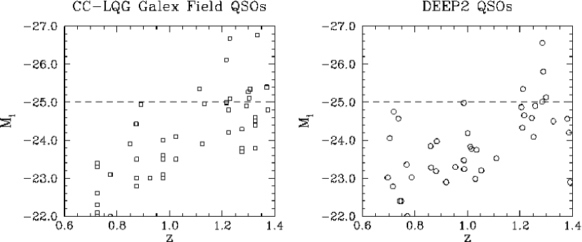
Figure 1: The distribution of QSO and AGN M_I magnitudes versus $z$ for our two GALEX fields (left, 2.2 deg²) and the four DEEP2 fields (right, 3 deg²; Coil et al. 2007). The QSO redshifts for the GALEX fields are from Clowes & Campusano (1991, 1994) and Newman (1999). Note that this plot does not include the objects from the photometric selected catalog of Richards et al. (2007), which includes another $\sim$40 QSO and AGN candidates to g$\sim$22.0 in the GALEX fields.

We observed part of the Clowes-Campusano LQG (CCLQG), which is the largest known LQG and has the most members. It contains at least 18 bright quasars at 1.2$<z<$1.5 and a spatial overdensity of 3 for B${}_{J}\,\leq\,20.0$ mag (Clowes & Campusano, 1991, 1994; Graham et al., 1995; Clowes et al., 1999; Schneider et al., 2007). The CCLQG covers $\sim$2.5 deg x 5 deg ($\sim$120x240 h^-2 Mpc² ) and is 590 h^-1 Mpc deep. It was discovered in a $\sim$ 25.3 deg² objective-prism survey using UK Schmidt plate data (plate UJ5846P or ESO/SERC field 927, Clowes & Campusano, 1991) and represents one of the largest known structures at $z>$1. It is 3$\times$ denser in bright (M${}_{I}<-25$) quasars compared to the DEEP2 fields (Fig. 1). Previous studies of the CCLQG showed an associated factor 3 overdensity of Mgii absorbers at 1.2$<z<$1.5 (Williger et al., 2002), which are linked to luminous galaxies (e.g. Steidel et al., 1997; Guillemin & Bergeron, 1997). There is also a foreground $z\sim 0.8$ LQG containing $\geq 14$ quasars and spanning $3.5^{\circ}\times 3^{\circ}$ on the sky. Studies of the galaxy populations in the LQGs showed $\sim$30% overdensities of red galaxies (I-K$>$3.4) at $z$=0.8 and z=1.2 (Haines et al., 2001, 2004). The galaxy colors are consistent with an evolved population, and form sheets which span a $\sim$40${}^{\prime}\times$34^′ subfield which we imaged deeply in VI using the CTIO Blanco 4m telescope (Haines et al., 2001, 2004). Smaller 5${}^{\prime}\times$5^′ SOFI subfields of near-IR imaging reveal three clusters at $z$ $\sim$ 0.8 and a pair of merging clusters at $z$ = 1.2 associated with a CCLQG member quasar (Haines et al., 2004).

2.2 Data

For this study we have imaged two slightly overlapping 1.2 degree fields within the CCLQG in the Far-UV (FUV; $\lambda_{eff}=1538.6$Å) and Near-UV (NUV; $\lambda_{eff}=2315.7$Å) filter bands, using the UV satellite GALEX (GALaxy Evolution eXplorer). The observations were part of the Guest Investigator program, cycle 1 proposal 35. The data used in this work consist of two $\sim$ 20000 s exposures in the FUV and two $\sim$ 35000 s exposures in the NUV filter band (Tab. 1). The pipeline reduction was done by the GALEX team, including the photometric calibration. We are able to detect point sources with SExtractor v.2.5.0 (Bertin & Arnouts, 1996) to m_NUV,FUV $\sim$25.5 mag. For further analysis we used the MAG_ISO parameter as measured by SExtractor, which gives total magnitude for the measured objects. For details see the SExtractor manual. A detailed description of the completeness analysis of the data can be found in § 2.4. Optical complementary data are from the Sloan Digital Sky Survey DR5 (June, 2006; Adelman-McCarthy et al., 2007), which is sensitive to limiting magnitudes of u$=22.0$, g$=22.2$, r$=22.2$, i$=21.3$, $z$$=20.5$. With the SDSS data, we have 7 band photometric information available for most of our UV-selected sample (see § 2.3). From the SDSS we obtained model magnitudes in the five filter bands, flux values, and spectroscopic and photometric redshift information. Since confusion of sources represents a significant effect in the GALEX data, we chose from the SDSS list the nearest primary object (as defined by the SDSS) within 4$.\!\!^{\prime\prime}$5 to match our UV detections.

2.3 Sample Selection

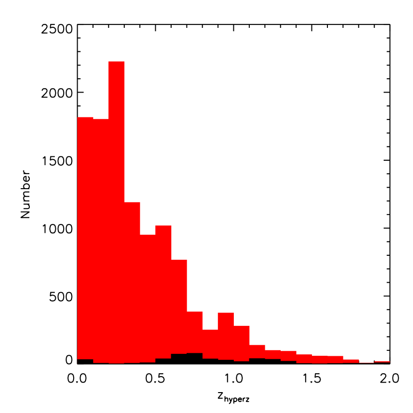
Figure 6: Photometric redshift distribution for all galaxies (left, red) and the LBG candidates (left and right black). We used a bin size for the redshift of $\delta$z=0.1. The red bars (left panel) represent the distribution in redshift for all galaxies for which we also have SDSS counterparts, while the black filled bars (left+right panel) display the photometric redshift distribution for the LBG candidates.

The analysis described in the following parts of the paper are based on a sample selected in the two UV filter bands of the GALEX data. The source catalog has been created using SExtractor v.2.5.0. The complete catalog consists of 15688 sources applying a detection threshold of 3.0 $\sigma$ and an analysis threshold of 1.5 $\sigma$, using the default convolution filter of SExtractor. Additionally, we also used weight maps as well as flag images to exclude bad regions at the edge of the GALEX images and saturated sources within our SExtractor search. The weight maps and flag images were constructed using weight watcher version 1.7 (Marmo & Bertin, 2008). A cross-correlation with the SDSS DR5 resulted in 14316 sources (matching radius: 4$.\!\!^{\prime\prime}$5). To clean our sample from false detections (e.g. bright star contaminations, reflections) we only selected objects which have a SExtractor extraction FLAGS $\leq\,2$ in the NUV filter, which resulted in a subsample of 13760 objects (final UV selected sample). For the star-galaxy discrimination in the sample we use the PhotoType values of the SDSS DR5, which works on the 95% level for object with r$\leq 22.2$ mag (Adelman-McCarthy et al., 2007). We selected all objects which were marked as GALAXY in the SDSS data, yielding 10982 galaxies. However, since the PSF of the GALEX data is relatively poor ($\sim$ 4$.\!\!^{\prime\prime}$5 for the FUV and $\sim$ 6″for the NUV filter), it is difficult to distinguish between real point sources (e.g. stars or quasars) and higher redshift extended sources which are point-like in the GALEX beam. Therefore, to reduce the contamination of our LBG sample with faint stars, we followed our more conservative approach. To account for smaller point like objects we also selected all objects which are marked as STAR and are located outside the mean stellar locus (MSL) as defined by Covey et al. (2007). For this selection we used the analytic fit for the MSL of Covey et al. (2007) in the g-i vs. r-i color-color space (see Fig. 2) and included all objects in our sample which have an offset to the MSL larger than the maximum offset indicated by the blue dashed lines. With these additional selection criteria, we ended up with a final sample of 11635 galaxy candidates with a photometric redshift distribution as shown in Figure 6 (red bars).

To identify $z\sim 0.5-1$ LBGs, we applied a FUV dropout technique, using the selection criteria of Burgarella et al. (2006) and including only objects classified as GALAXY by the SDSS DR5 or outside the MSL and with m${}_{NUV}<23.5$ mag and m${}_{FUV}-$m${}_{NUV}>2$ mag. This resulted in a final sample of 1263 LBG galaxy candidates (618 deg^-2), which is only about half the detection rate of Burgarella et al., who found 1180 LBG candidates per deg² in the CDF-S. Without these additional selection parameters our selection would have resulted in a sample of 2566 LBG candidates or 1256 deg^-2, which is comparable to the results of Burgarella et al.. However, unlike Burgarella et al., we only have 7 band GALEX+SDSS photometry as opposed to their much wider UV to mid-IR wavelength coverage and higher resolution imagery. Therefore, to reduce the contamination of our LBG sample with faint stars, we followed our more conservative approach.

2.4 Completeness and Confusion

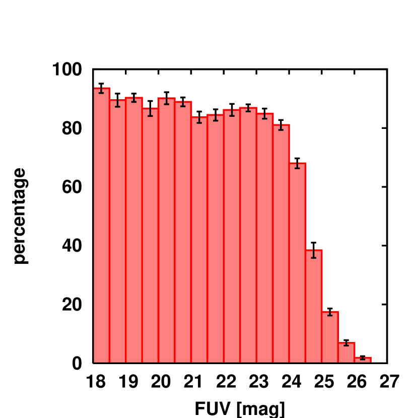
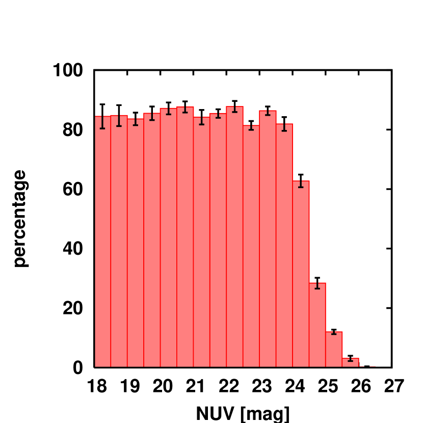
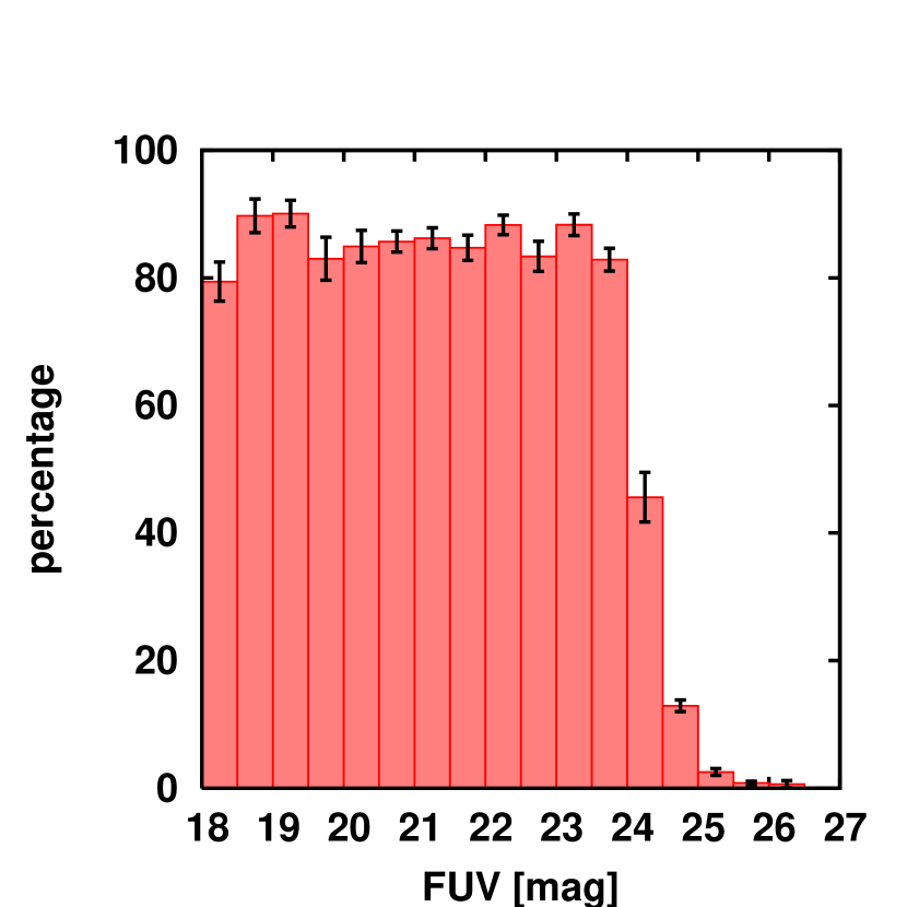
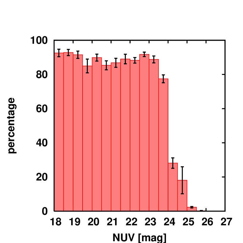
Figure 3: Results of the completeness simulations for the northern (upper row) and southern field (lower row) in the FUV (left column) and NUV (right column) filters. The marginally low values for the detection efficiency at AB$<$24.0 can be explained by confusion due to the large GALEX PSF.

We used a Monte Carlo-like approach to check the completeness of galaxy counts in the FUV and NUV filter bands. The process relies on a well-known artificial sample of galaxies. To keep the basic image information (e.g. noise pattern, pixel size, PSF) of the original data, we simulated the artificial galaxy sample as follows. We first removed all sources detected by SExtractor from the images, to get a source-free image with the real observed background. This was done using the SExtractor check-image (CHECKIMAGE_TYPE = -OBJECTS). In the cleaned images we then placed a list of simulated galaxies constructed by running the IRAF task gallist. We created a list of 2000 synthesized galaxies randomly placed in a $\sim$0.7 deg² field. To simulate the artificial galaxy sample, we chose a luminosity distribution based on a power law with an exponent of 0.1. The simulated galaxy list consists of objects with total magnitudes between 14 and 25.5 mag and redshifts out to $z$ = 1.3. To create the galaxies in the source-free GALEX images, we applied the IRAF task mkobjects. This procedure resulted in a well-defined data set with a known galaxy sample which we could use for further analysis. We then photometrically analyzed the artificial galaxies and derived their total magnitudes using the galaxy fitting routine galfit (Peng et al., 2002) on the simulated data. In the final step, we searched the images for galaxies with SExtractor by applying the same extraction parameters as for our science data (see § 2.3), and compared the resulting list with the input list to compute detection efficiencies. We repeated this procedure ten times and calculated the mean and standard deviation for the detection efficiencies (see Fig. 3). For all four cases (FUV, NUV data for the northern and southern fields) our detection efficiency is around 80-90% for objects with total magnitudes down to 24 AB. The detection efficiency decreases to $\sim$60% at 24.5 ABmag for the northern FUV and NUV images and 45-30 % for the southern images. For objects with total magnitudes fainter 24.5, the detection efficiency drops below 40% for the northern and below 20% for the southern field. The marginally low efficiencies (only 80-90%) for the bins brighter than 24 AB can be explained by blending effects due to confusion resulting from the large pixel size of GALEX (1$.\!\!^{\prime\prime}$5) and the large PSF in the FUV ($\sim$5″) and NUV filters ($\sim$ 6$.\!\!^{\prime\prime}$7).

We therefore checked the GALEX detections for multiple counterparts using higher resolution optical images obtained at the CFHT with Megacam. The images reach limiting magnitudes of r=27 and z=25, with a mean image quality of $\sim$1 arcsec in both filters (for more details see Haberzettl et al., 2009). Confusion can effect the photometry either by increasing the flux of detected objects directly or by changing the background estimates in the surrounding of the detected objects if the backround is estimated locally. Since we derive a global estimate of the background within SExtractor by using a mesh size of 64 pixels (significantly larger than the PSF), this effect should be small and can be neglected. More important is the change in photometry from additional objects within one FWHM. We therefore matched all sources in the NUV-, r-, and z-band using a radius of 3^′′ diameter, which covers a slightly larger area than the 5$\farcs$4 FWHM of the GALEX NUV data. Our analysis show that 19% of the complete sample has 2 or more counterparts to r$\sim$27. Restricting our study to counterparts with r$\leq 24.5$, the multiple counterpart fraction decreases to 16%. For the LBG candidates with NUV$\leq 23.5$, we found 2 or more counterparts for 22% of the sample (r$\leq$24). Although these values for confusion are slightly higher then previously reported (e.g. 13% Bianchi et al., 2007), we do not correct our sample using deconvolution methods, since our results are based on averages over samples of galaxies. The effects of confusion will be minor, compared to the scatter in our SEDs (details in §4-5). To this point, we did not restrict optical counterpart colors. If we restrict optical counterparts to r-z$\leq$0.5 (or f${}_{z}\geq$1.5 f_r) which means the objects are likely to be either relatively old ($\gtrsim$5 Gyr) or dust reddened and in both cases have significantly reduced UV-fluxes, the fraction with $\geq$2 counterparts reduces to 16% for the complete sample (NUV$\leq$23.5) and 10 % for the LBG subsample.

Additional information about confusion results from the number of sources per beam (beams per source). We followed the approch by Hogg (2001) as used by Burgarella et al. (2007). Restricting the galaxy sample to NUV $\leq$ 23.5 results in (s/b)${}^{3\sigma}_{conf}$ = 0.0038 sources per beam (265 beams per source). This is much shallower than the 3$\sigma$ confusion limit of (s/b)${}^{3\sigma}_{conf}$ = 0.063 or 16 beams per source reported by Burgarella et al. (2007) indicating that confusion will not effect our results significantly.

$$(s/b)^{3\sigma}_{conf}~{}=~{}\frac{N_{sources}}{\Omega_{GALEX}/\Omega_{beam}}$$ (1)

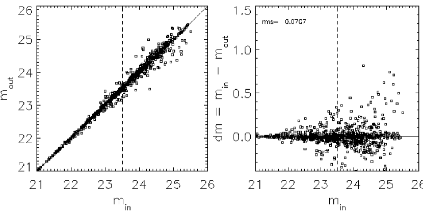
Figure 5: Effect of confusion on photometric results of NUV GALEX data. Comparison of magnitudes before (m_in) and after placing additional artificial galaxies in the field (m_out). For galaxies with m${}_{in}\leq$23.5 (reflecting the selection criteria used for the LBG candidate sample) the change in magnitude is relatively small with a rms for the offset dm_rms = 0.0707.

To test the effect of confusion on our photometry, we simulated GALEX NUV images using SkyMaker 3.1.0 and STUFF 1.17 developed by Bertin & Fouqué (2007). The galaxy distribution was created using STUFF 1.17 default parameters for a 1024$\times$1024 image and represent the galaxy sample of interest for which we wish to measure the photometry. The instrument specific parameters (e.g. pixel size, mirror size) were set to GALEX specifications. The galaxy distribution includes objects with 18$\leq$MAG_LIMITS$\leq$26.5. We then created a simulated image with SkyMaker for a $\sim$33 ksec exposure using the GALEX NUV PSF. The comparison in number density and brightness distribution between the real and the simulated GALEX NUV data shows good agreement (Fig. 4). We added a uniformly distributed sample of 100,000 artificial background galaxies to the data, simulated using IRAF tasks gallist and mkobjects. The sample was made using a power law distribution $dN\sim m^{-\beta}$ with $\beta=0.6$, restricted to 18 $\leq m\leq$ 28.5 including background galaxies down to the 1% flux level of out NUV magnitude limit. Comparison of SExtractor catalogs with and without the synthetic galaxies shows no significant effects on the photometric results for objects with $m\leq 23.5$ (see Fig. 5). The rms for the change in m_iso is dm_rms = 0.0707 mag, including objects which have $\rm dm<0$ resulting from changes in the deblending during the SExtractor search and/or overall higher background level due to the high number of background galaxies. The rms of change in m_iso accounting only for objects with $\rm dm\geq 0$ is dm_rms = 0.0784. This is small compared to the NUV scatter in the averaged SEDs, which can be as high as 1.5 mag. We conclude that our catalogs are 80 - 90,% complete down to m_NUV = 24 AB. For LBG candidates we are 40 - 60 % complete to AB_NUV = 24.5.

3 Photometric redshifts

We used seven band photometry from the two GALEX (FUV+NUV) and the five SDSS DR5 (u,g,r,i,z) filter bands for photometric redshifts of our final UV selected sample, applying the algorithm from hyperz v1.1 (Bolzonella et al., 2000). The variance of Lyman-$\alpha$ opacity in the intergalactic medium (Massarotti et al., 2001) produces a negligible effect at these redshifts. The redshift determination is done by cross-correlating a set of template spectra to the colors of the sample galaxies. In the current version of hyperz we used a set of four template spectra from Bruzual & Charlot (2003), consisting of an elliptical, Sc, Sd galaxy, and star-burst. The resulting redshift distributions for the total galaxy and LBG candidate samples are shown in Fig. 6.

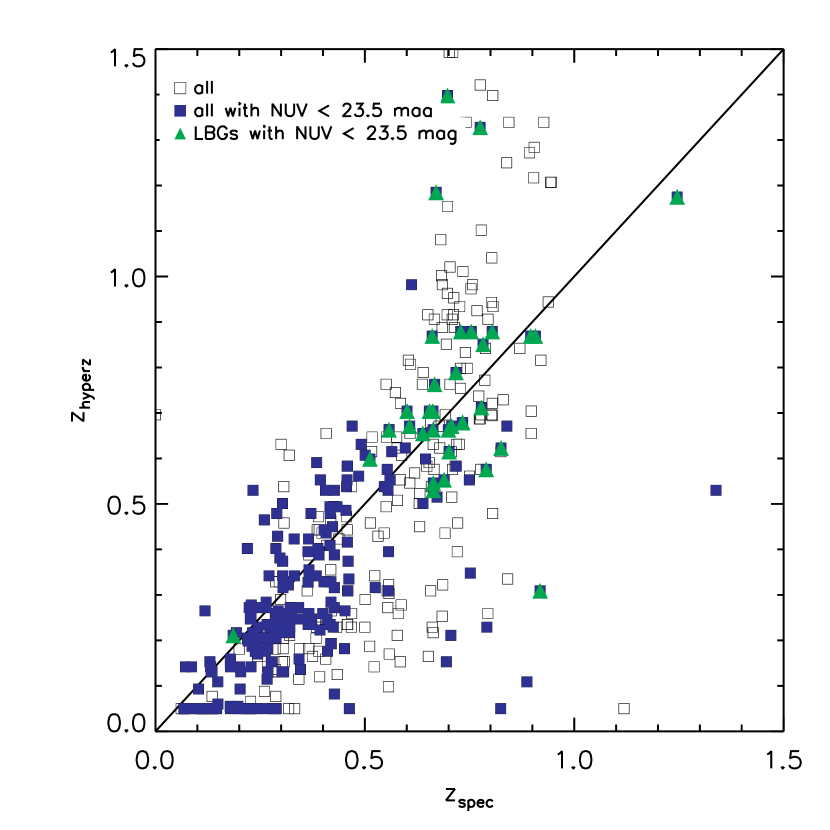
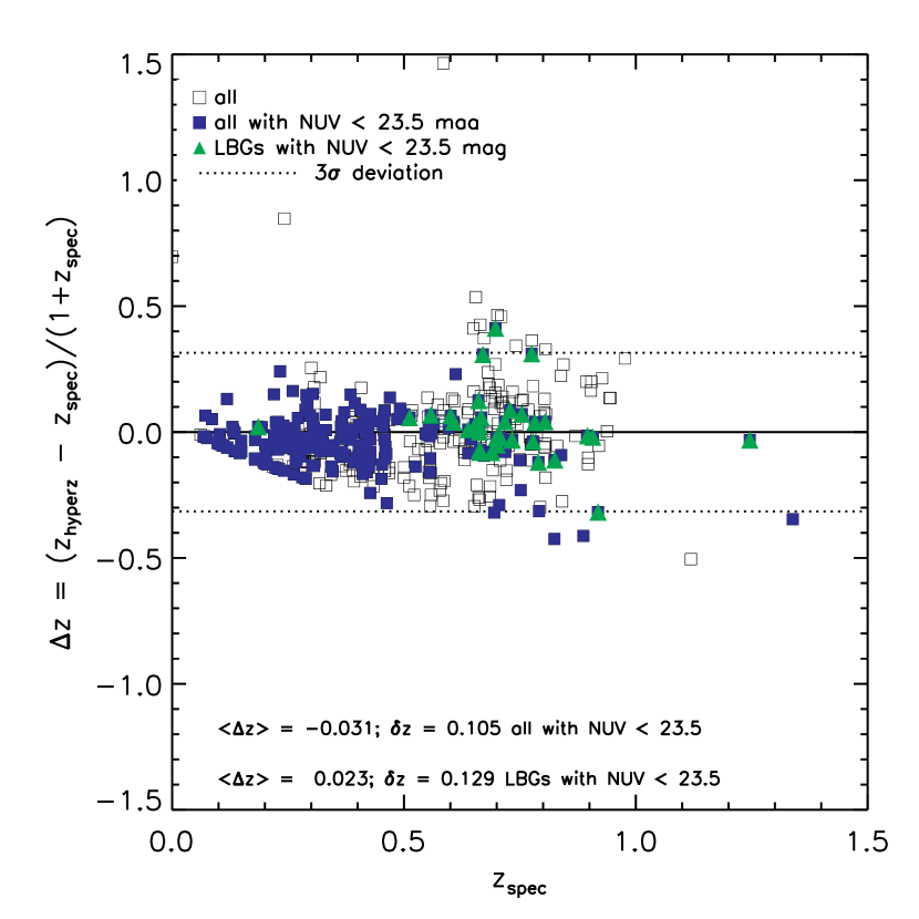
Figure 8: The left panel shows the comparison of our photometric redshifts $z_{hyperz}$ obtained using 7 band photometry (FUV,NUV,u,g,r,i,z) to spectroscopic redshifts which we obtained for a subsample of 448 galaxies. Blue triangles are galaxies with m${}_{NUV}\,\leq\,$23.5 mag. Green triangles represent the LBG candidates with m${}_{NUV}\,\leq\,$23.5 mag. The right panel shows the residuals $\Delta$z using the same color schemes. From the right panel we see that the number of catastrophic outliers is relatively small (all 2.6% and LBG candidates 5.9%) for galaxies with m${}_{NUV}\,\leq\,$23.5.

To get information about the accuracies of our photometric redshifts estimation, we compared the resulting photo-z’s of the final galaxy catalog with a subsample of 448 galaxies for which we have spectroscopic redshifts (see Figs. 7 and 8). The spectra were observed using the IMACS mult-object spectrograph at the 6.5 m Baade Magellan telescope (Harris et al., 2009). The spectroscopic subsample covers 0.06$<$z$<$1.34 with a mean redshift of $\left<z\right>$ = 0.48$\pm$0.23. The photometric redshift accuracy decreases significantly for objects with m${}_{NUV}>$23.5 mag (Fig. 7), and the standard deviation $\sigma_{\Delta z}$ increases from 0.105 (0.129 for LBG candidates) to 0.203 (0.195 for LBG candidates). We therefore restricted our analyses to objects brighter than m_NUV = 23.5 (blue and green triangles in Figs. 7 and 8). This leaves a more conservatively selected sample of the 462 LBG candidates. For our spectroscopic subsample we derived mean offsets of $\left<\Delta z\right>=-0.031$ for the whole bright sample (blue + green triangles) and $\left<\Delta z\right>=0.023$ for the LBG candidate sample (green triangles). We therefore see no significant systematic offsets. The fraction of catastrophic outliers ($\Delta z\,>\,3\sigma$, Fig. 8) for bright objects (m${}_{NUV}\leq$23.5) is about 2.6% (5.9% for LBG candidates).

Using our GALEX plus 7 band SDSS photometry, we are able to obtain unbiased photometric redshifts with well defined uncertainties for objects with NUV$\leq$23.5 for both the complete galaxy as well as the LBG sample. Hence our LBG selection should be reasonably robust, given the depth in redshift of our four galaxy samples (see § 4 and 5) which is 2-3 $\sigma$ for the derived uncertainties of our photometric redshifts. We therefore assume no significant impact from the relatively large photo-z scatter on our results.

A listing of our LBG sample is in Table 2, available in the electronic edition of this paper. We also provide information on the LBGs on our team website.

4 SED fitting

To constrain the evolution of galaxies in the dense quasar environment of the two LQGs, we compared averaged SEDs built out of the photometric measurements of our sample galaxies to model SEDs derived from the synthesis evolution model PEGASE (Fioc & Rocca-Volmerange, 1997). We used a library of several thousand PEGASE spectra from an extended parameter study to probe the star formation histories (SFHs) of a sample of Low Surface Brightness (LSB) galaxies (Haberzettl et al., 2009).

We made stacked SEDs of our LBG candidate samples (§ 5) from the GALEX+SDSS 7-band photometry. The stacked SEDs were constructed for four different redshift bins over $0.5\leq z<0.7$ (foreground sample FG1), $0.7\leq z<0.9$ (LQG0.8), $0.9\leq z<1.2$ (foreground sample FG2) and $1.2\leq z<1.5$ (CCLQG). To reduce the influence of extreme objects (e.g. redshift outliers, mis-identified stars) we applied upper flux limits for the averaged SEDs in all filter bands, excluding iteratively all objects which have fluxes more than 3$\sigma$ from the mean flux. Additionally, we only used objects which have non-negative fluxes in all filter bands. The errors for the mean fluxes in the single filter-bands are represented by their standard deviations. By fitting the model SEDs to averaged low resolution spectra of our LBG sample, we were then able to obtain SFHs and luminosity-weighted ages (results described in § 5). The model SED library contains spectra calculated for different star formation laws (SFLaws), star formation rates (SFRs) and extinction geometries. The model SEDs were constructed accounting for consistent chemical evolution. This is a more realistic approach than the use of simple stellar populations (SSPs) with fixed metallicities, giving us the advantage that the metallicity is not a free parameter. Therefore, we preferred PEGASE over other models as for example the widely used Bruzual & Charlot models (Bruzual & Charlot, 2003). We chose four different SFLaws including star-burst scenarios, constant, exponentially decreasing, and power law SFRs. The best matching SEDs were derived by performing a $\chi^{2}$-fit between model and measured SEDs. To judge the quality of our SED fit results we compare the reduced $\chi^{2}$-values against the ages of the fitted SEDs (Figs. 11a, 11b, 11c, 11d), which is the parameter of main interest to us. From these plots we estimate the 1$\sigma$ uncertainties by comparing $\chi^{2}$ for every SED to $\chi^{2}_{min}+1$.

Since we are analyzing samples of LBG candidates, we set the measured fluxes in the GALEX FUV band to zero for those redshift bins where the FUV-band would be below 912 Å  in the rest frame. We normalized the flux of both modeled and measured SEDs with respect to the rest frame flux in z-band, and redshift-corrected the measured SEDs according to the mean redshift of the group to which each of the averaged LBG spectra belongs. We next describe the stacked SEDs and results.

5 Lyman Break Galaxy candidate sample

Our NUV$<$23.5 criterion gives a conservative sample of 462 LBGs, for which our 7-band UV-optical photometric redshift distribution is shown in the two histograms in Fig. 6. The red filled bars represent the photometric redshift distribution for the whole galaxy sample, while the LBG candidate sample is represented by the black filled bars. From the right panel we see that most (405) of the LBG candidates have photometric redshifts $z\geq$0.5. The mean photometric redshift of the LBG candidate sample is $\left<z_{LBG}\right>=0.86\pm 0.45$, compared to the mean of the final galaxy sample of $\left<z_{galaxies}\right>=0.41\pm 0.35$. Only 60 LBG candidates lie between 1.2$\leq$z$<$1.5 and are associated with the CCLQG. We mainly probe the foreground LQG (LQG0.8) at 0.7$\leq$z$\leq$0.9 (117 LBG candidates). The FUV dropout technique effectively identified $z\geq$0.5 galaxies: 88 % are at $z\geq$0.5.

For further analysis, we have divided the LBG candidate sample into four redshift bins (Table 3): 0.5-0.7 (FG1 sample), 0.7-0.9 (LQG0.8 sample), 0.9-1.2 (FG2 sample), and 1.2-1.5 (CCLQG). For each redshift bin, we selected two subsamples for intrinsically bright and faint LBG candidates according to their absolute brightness in the GALEX NUV filter band (rest frame FUV). For the selection we used the values of M${}^{*}_{NUV}$ from Arnouts et al. (2005, M${}^{*}_{NUV}$ = -19.6, -19.8, -20.0, and -20.2 from low to high redshift) consistent with the four redshift bins, and K-corrected the measured NUV magnitudes using the kcorrect software v4_1_4 of Blanton et al. (2003, see also Fig. 9). The bright and faint subsamples consist of 3 to 69 candidates. For the FG2 and CCLQG sample, we were not able to detect any faint (M${}^{*}_{NUV}\geq$-19.8 mag or -19.6 mag) LBG candidates.

Finally, we divided our LBG candidate sample into red and blue subsamples using the MSL in the g$-$i vs. r$-$i color-color diagram. For all redshift bins, this selection resulted in a larger red than blue subsample and is a first indication that our LBG samples are dominated by either dusty or more evolved galaxies.

5.1 Star Formation History

We used the SED fits of § 4 (Figs. 10a,b) to constrain the LBG candidate star formation histories. Although $\chi^{2}$-fits did not result in unique solutions (see Figs. 11a,b) the best fitting SEDs give luminosity-weighted ages between 3.5 - 6 Gyr for the dust-free models and 1.0 - 4.0 Gyr for models including dust. Results for the SED fitting are summarized in Tables 4-7 and explained in more detail below.

The best fitting SFH for the FG1 sample, consisting of 64 LBG candidates with -20.38$\leq$M_NUV$\leq$-18.85, is described by an exponentially decreasing SFR (decay time $\tau=0.5$ Gyr) after 6 Gyr for the dust-free and a star-burst after 2.5 Gyr for dust-containing models using an edge-on disk geometry. Subdividing FG1 into a bright (M${}_{NUV}<$ -19.6) and faint (M${}_{NUV}\geq$ -19.6) subsample resulted in the same SFHs for the dust-free model. For the models including dust the bright subsample is best represented by a 4.0 Gyr old exponentially decreasing SFR (decay time $\tau=1.0$ Gyr) assuming a face-on disk geometry for the dust distribution. The faint subsample is best described by a star-burst scenario after 2.5 Gyr using an edge-on disk geometry. The dust-free and dusty models for the complete sample and the dust-free models for the bright and faint subsamples are both relatively well constrained, allowing for only one solution within the $\chi^{2}+1$ limit. The ages derived from the dusty models for the bright subsample range between 2.5 and 6 Gyr for a star-burst and exponentially decreasing SFRs with different dust geometries. The faint subsample is fitted with 2.5 Gyr old star-bursts with spherical, face-on and edge-on dust geometries.

The fits for the FG2 sample ($0.9\leq{\it z}<1.2$) resulted in SFHs with slightly younger luminosity-weighted ages. The total sample included in the fits consists of 35 LBG candidates with -22.28 $\leq$ M_NUV $\leq$ -20.38 and could be best fitted by a constant SFR after 6.0 Gyr for the dust-free (only fit acceptable) and a burst scenario after 1.0 Gyr for the dusty model. The dust is assumed to be distributed with a face-on disk geometry. For this redshift slice we were not able to detect a faint subsample. The acceptable SEDs including dust result in star-bursts with ages ranging between 1 to 1.4 Gyr using the five different dust geometries in the library (spherical, inclination averaged, face-on, 45^∘ inclined, and edge-on).

The foreground large quasar group (LQG0.8 sample) consists of 73 LBG candidates with absolute magnitudes -20.97$\leq$M${}_{NUV}\leq$-19.67. The SFH is best described by an exponentially decreasing SFR (decay time $\tau=0.5$ Gyr) after 3.5 Gyr for the dust-free and a star-burst after 1.4 Gyr for the dusty models (edge-on disk). For the bright (M${}_{NUV}<$ -19.8) and faint (M${}_{NUV}\geq$ -19.8) subsamples the SFHs were best fitted by exponentially decreasing SFRs (decay time $\tau=0.5$ Gyr) after 3.5 Gyr (bright) and constant SFR after 6 Gyr (faint) assuming dust-free models. The models including dust extinction were best fitted by a star-burst after 1.4 Gyr (bright) and an exponentially decreasing SFR (faint, decay time $\tau=0.5$ Gyr) after 3.5 Gyr respectively. The dust distributions are assumed to represent edge-on (bright) and 45^∘ inclined disk (faint) geometries. The dust-free models for the complete, bright, and faint subsamples are well constrained, allowing for one fit within the $1\sigma$ limit. For the models including dust, the acceptable fits result in ages between 1.2 and 3 Gyr for the complete and 1.2 and 6 Gyr for the faint susbample using a star-burst for the complete and an exponentially decreasing SFR for the faint subsample including all dust geometries. The bright subsample is well represented by exponentially decreasing SFR after 3.5 Gyr using an inclination averaged or 45^∘ disk dust geometry.

The CCLQG LBG sample only consists of 25 LBG candidates with absolute magnitudes M${}_{NUV}\geq$ -21.34. Therefore, we could only derive SFHs for the M$>$M^∗ LBG candidates. For dust-free models, the SFH is best described by a constant SFR after 6 Gyr (only acceptable solution), while for the models including extinction the best fit is from a star-burst after 3 Gyr (spherical dust geometry). The dusty models also allow for solutions ranging from 1.6 to 4 Gyr for the age, using star-bursts with all five possible dust geometries.

The SFHs for all subsamples resulted in significantly older best fitting ages compared to the results of Burgarella et al. (2007). The ages derived here correspond to formation redshifts between 1.5 and 5, which is consistent with the peak of the luminosity density in the Universe (e.g., Nagamine et al., 2000; Sawicki & Thompson, 2006). Although we have no direct measurement of the dust content for our LBG candidates, the dusty models fit best the LBG candidate samples in the two LQGs (LQG0.8 and CCLQG) indicating that dust plays a non-negligible role.

The relatively large red to blue subsample sizes and the old ages for the LBG candidate samples indicate that the populations are dominated by evolved redder galaxies in comparison to the LBG sample of Burgarella et al. (2007). The best fitting model SEDs give mean luminosity-weighted ages between 1.2 and 6 Gyr (see Fig. 10c and 10d), with similar results for blue and red subsamples. Dusty model estimates range over 1.0–5 Gyr. The acceptable range of SED fits for the models including dust allows for ages as young as 0.9 Gyr (Figs. 11c,d).

5.2 Luminosity Function

We estimated the luminosity functions (LFs) for our LBG candidate samples in the four different redshift bins using 1/V_max (Schmidt, 1968) We used k-corrected NUV magnitudes to estimate rest frame FUV fluxes, covered by the GALEX NUV filter-band at our redshift intervals.

For the 1/V_max method, we followed the approach used by many other studies (e.g. Eales, 1993; Lilly et al., 1995; Ellis et al., 1996; Arnouts et al., 2005; Willmer et al., 2006)

$$\Phi(M,z)=\sum_{i=1}^{N}\frac{\omega_{i}}{V_{max,i}\Delta m}$$ (2)

where $\omega_{i}$ represents the weighting factor accounting for incompleteness. The maximum volume a galaxy can be observed and still satisfy the sample selection criteria is described by (Hogg, 1999)

$$V_{max}=\left(\frac{c}{H_{0}}\right)^{3}d\Omega\left(\int_{z_{l}}^{z_{u}}{\frac{dz}{\sqrt{\Omega_{m}(1+z)^{3}+\Omega_{\Lambda}}}}\right)^{3}$$ (3)

For the integration limits we used the fixed limits $z_{l}$,$z_{u}$ of our four different redshift intervals. We calculated the errors for the LF using

$$\sigma_{\Phi}(M,z)=\sqrt{\sum_{i=1}^{n}\left({\frac{\omega_{i}}{V_{max,i}\Delta m}}\right)^{2}}$$ (4)

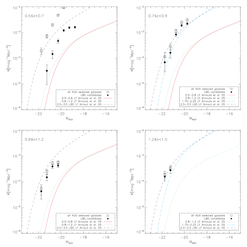
Figure 12: Luminosity Functions (LFs) for the LBG candidate samples (filled diamonds) and the all NUV selected galaxies (open squares) in the four different redshift bins. The LFs were derived using the 1/V_max-method. For comparison we plotted LFs for different redshift intervals and selection criteria of Arnouts et al. (2005).

The results are compared to parameterizations of the Schechter function as derived by Arnouts et al. (2005, see Fig. 12). For the FG1,FG2 and LQG0.8 samples we were able to cover the LF down to roughly M^∗. For the CCLQG at 1.2$\leq z<$1.5 we were only able to derive the LF for LBG candidates down to roughly 3M^∗, including only two bright magnitude bins.

The Schechter parameterization derived by Arnouts et al. (2005) for all types of NUV-selected galaxies in Fig. 12 is exceeded by the data, which implies that in all four redshift bins the LBGs are over-abundant for their redshift. In the two LQGs at $z\sim$0.8 and $z\sim$1.3 the volume densities of the LBGs are consistent with Arnouts et al. parameterization of the LFs at 1.75$<z<$2.25 or LBGs at 2.5$<z<$3.5. In comparison to the two foreground samples (FG1 and FG2) we also find an increase in the abundances of LBGs for the two LQGs. Although the uncertainties in photometric redshifts are large and there is some blending with the less dense foreground regions, there is a clear indication for higher densities of star forming galaxies in the two LQGs from the LFs. We have a sample of 112 LBG candidates for the foreground LQG and 117 for the CCLQG. Since the volume decreases by 43% from $0.7\leq z<0.9$ to $1.2\leq z<1.5$, we estimate an overdensity of 46$\pm$7% or 2.6$\sigma$ for the CCLQG compared to LQG0.8. The overall higher volume densities for LBGs in all four redshift bins may at least partly be due to our LBG selection criteria which includes galaxies which are relatively evolved.

5.3 LBG concentrations and LBG-quasar correlations

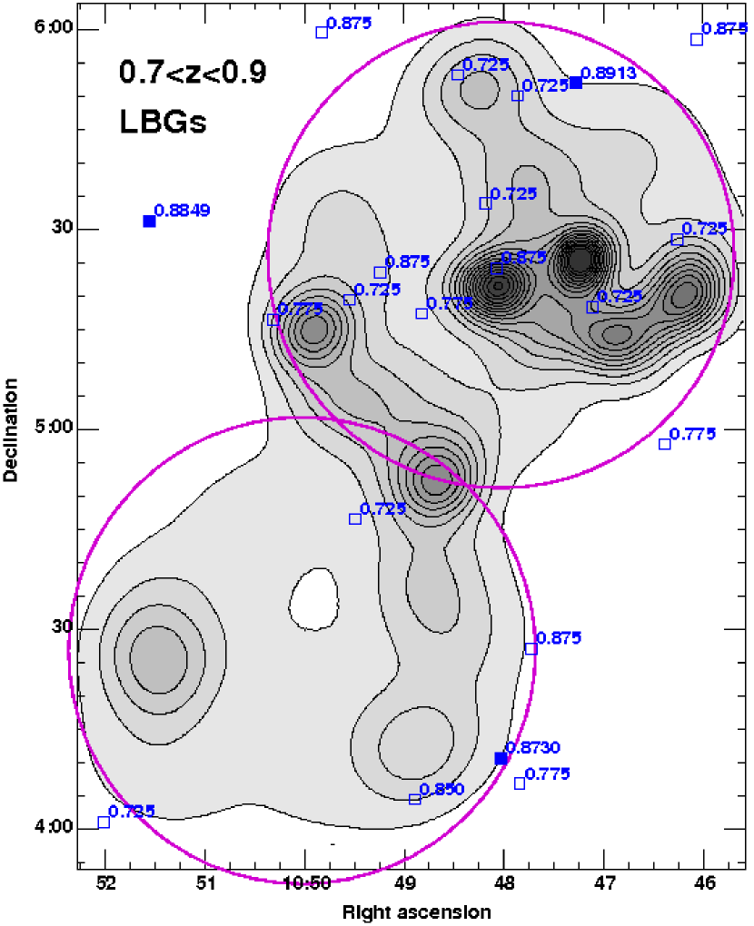
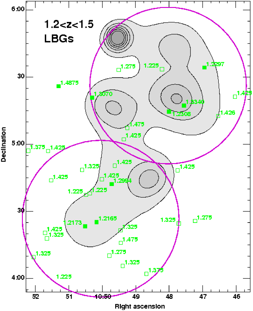
Figure 13: Density plot for the LBGs in the two LQGs at $z\sim$0.8 (left with blue/dark quasar labels) and $z\sim$1.3 (right with green/light quasar labels). Filled squares represent spectroscopic and open photometric quasar samples. The two GALEX pointings are indicated by the large circles. The lowest density contour represents a density of 20 LBGs deg^-2 with a separation of 20 LBGs deg^-2 between contours. Both LQGs show concentrations and structures of LBGs (center of the northern and southeast in the southern GALEX field).

In Figure  13 we show the density maps of LBGs photometrically-selected to be at $0.7<z<0.9$ (left panel) and $1.2<z<1.5$ (right panel). The LBG density maps were computed using a variant of the adaptive kernel method (Silverman, 1986) in which each LBG in the redshift slice is represented by a Gaussian kernel centered on the LBG. Following Haines et al. (2007), we define the width of the Gaussian kernel to be equal to the distance to the third nearest neighbor LBG within the same redshift slice, and then calculate the local density at each point as the sum of the Gaussian kernels. The isodensity contours in each plot are linearly spaced at intervals of 20 LBGs deg^-2, the first contour corresponding to an LBG density of 20 deg^-2.

A number of distinct structures appear in the $z\sim 0.8$ LQG. For the CCLQG at $z\sim$1.3 we were only able to detect the brightest LBG candidates with L_NUV$\geq$1.5$\times$10¹²L_⊙. Several studies have indicated that at $z<0.5-1$, quasars avoid both the highest density galaxy regions and the field, instead preferentially populating cluster outskirts (e.g. Söchting et al., 2002, 2004; Kocevski et al., 2008a). Such behavior is also suggested in Fig. 13.

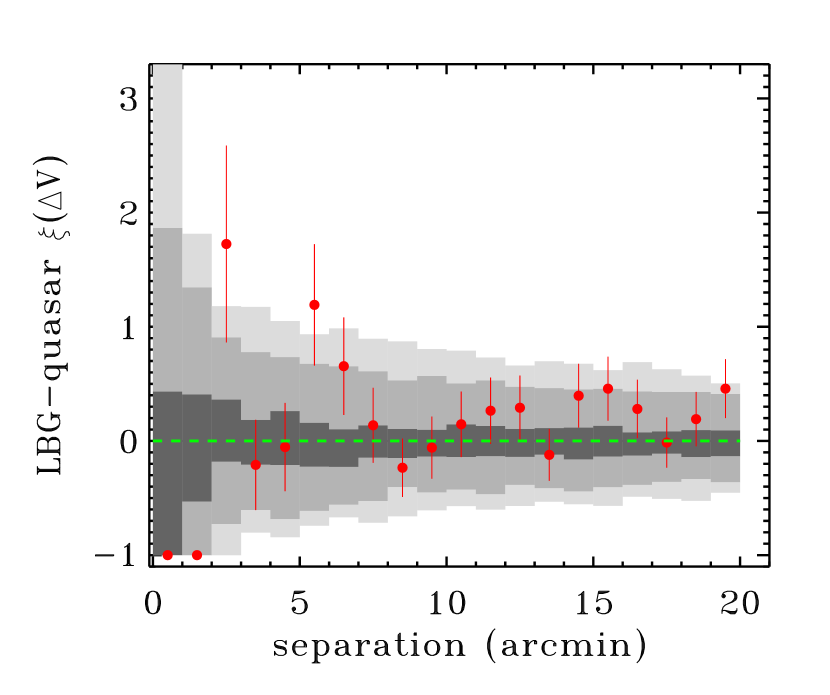
Figure 14: Two point correlation function for LBGs (117) and quasars (17) at $0.7<z<0.9$, within the two GALEX fields. This redshift slice provides the largest combination of LBG-quasar pairs. Shaded regions denote 68, 95, 99% confidence limits from 10,000 Monte Carlo simulations of sets of 17 random quasar RA and DEC placements in the observed area. Error bars show example $1\sigma$ Poissonian errors. At $z=0.8$, 1 arcmin corresponds to 0.45 local-frame or 0.81 co-moving Mpc. There are no LBG-quasar pairs within 2 arcmin of each other. The signal at 2-3 arcmin arises from 10 pairs. None of the 10,000 simulations had more than 9 in that bin, and we estimate the significance at $3.3\sigma$. The signal at 5-6 arcmin arises from 17 pairs. None of the 10,000 simulations had more than 15 in that bin, and we estimate the significance at $3.1\sigma$. However, the $\sim 1.8\sigma$ overdensity at 6-7 arcmin separation, and the lack of an overdensity at 3-4 arcmin, implies that the overdensity at separation 5-7 arcmin is more robust.

We can test for quasar-LBG correlations in redshift slices using our photometric redshift estimates, for comparison with higher redshift AGN-LBG correlations from Adelberger & Steidel (2005). The largest number of pairs would arise for $0.7<z<0.9$, which contains 17 quasars and 117 LBGs. We calculated the nearest neighbor distribution in angular distance in arcminute bins (1 arcmin is 0.8 co-moving Mpc), and compared it with 10000 randomly placed sets of 17 quasars within the GALEX fields. Results indicate mild ($\sim 2\sigma$) overdensities at 2–6 arcmin or $\sim 1.6-4.8$ co-moving Mpc (Fig. 14). This is consistent with the LBG-AGN correlation length of Adelberger & Steidel, and a factor of at least 3 smaller than the overdensities around quasars measured by the proximity effect at $2.1<z<3.3$ (D’Odorico et al., 2008). Although it could be expected that $z\sim 1$ LBGs would be less massive than their $z\sim 3$ counterparts due to downsizing, our sample appears to be dominated by massive galaxies and could well be similar to the Adelberger & Steidel sample. If quasars have similar regions of enhanced density around them at $z\sim 0.8$ as at $2.1<z<3.3$, then $z\sim 0.8$ LBGs would fall in regions of heightened density, but not so high as quasars.

6 Summary and Conclusions

We present first results from the Clowes-Campusano LQG Survey, a 2 deg² multi-wavelength approach to study one of the largest structures with high quasar density in the high redshift Universe (z$\sim$1), the Clowes-Campusano Large Quasar Group. The observations also covered a second LQG in front of the CCLQG at z$\sim$0.8. Our data set includes GALEX FUV+NUV images covering a 2 deg² field and optical photometry of the NUV selected sample from the SDSS DR5. With GALEX data, we reached a detection efficiency ranging between 80 – 90 %. The detection efficiency declines at m${}_{FUV,NUV}\,=\,24$ due to confusion and incompleteness. Using the FUV-dropout technique, selection criteria adopted from Burgarella et al. (2006) and object classification from SDSS DR5, we were able to select a sample of 1263 star forming LBG candidates down to m${}_{NUV}=24.5$. Since photometric redshift uncertainties increase significantly for galaxies with m${}_{NUV}\geq$23.5, we restricted further analysis to a subsample of 462 LBG candidates with m${}_{NUV}\leq$23.5. We derived 7-band photometric redshifts with accuracies $\sigma_{\Delta z}$ = 0.105 for all galaxies with $m_{NUV}<23.5$ and $\sigma_{\Delta z_{LBG}}$ = 0.129 for the corresponding LBG candidates. The mean photometric redshift of the LBG candidate sample is $\left<z\right>=0.86\pm 0.45$, and the majority of LBGs are at $z<1$, so we mainly probe the foreground LQG. We derived star formation histories for bright and faint LBG candidate subsamples, and found relatively old best fitting luminosity-weighted ages of 1.0-6 Gyr for models with and without dust. Compared to the results of Burgarella et al. (2007), who estimated ages in the range of 250-500 Myr, our best fitting ages are significantly older. This indicates that our sample is dominated by more evolved, redder (and likely more massive) LBG candidates. Dividing the LBG candidates into blue and red subsamples using the mean stellar locus led to a similar conclusion. The best fitting SEDs for the blue and red subsamples yielded consistent ages ranging between 1.0 and 6 Gyr. Due to the high uncertainties of the SFHs resulting from the use of broad band photometry and the large scatter of the averaged SEDs, it is important not to over-interpret the results for the luminosity-weighted ages. Our sample of LBG candidates includes only the most luminous galaxies which formed stars over a long period, resulting in a significant population of old red stars to counterbalance the young stars which produce the Lyman break. The faint LBGs in the LQG0.8 subsample show marginally larger luminosity-weighted ages T_L. A possible explanation is lower SFRs in the fainter subsample, which is supported by evidence for a larger red and more evolved population of LBGs in LQG0.8 compared to FG1 and FG2, which are not coincident with LQGs.

Possible effects of different environment densities can be more clearly observed in the luminosity function for the four redshift slices. The LFs for LBG candidates in the two LQGs show an increased volume density of star forming galaxies compared to results of less dense regions in the CDF-S (Arnouts et al., 2005). The LBG LF in the foreground LQG (LQG0.8) is consistent with their parameterization of the Schechter function corresponding to 1.75$<z<$2.25. Although we only have two luminosity bins for the CCLQG, it also shows evidence for an overdensity (more consistent with a population at 2.5$<z<$3.5). Both redshift slices containing LQGs have larger relative overdensities than the two redshift slices which do not contain quasar overdensities. We derived a sample of 112 LBG candidates for the foreground sample at 0.5$\leq z<$0.7 (FG1) and 117 LBG candidates for the foreground LQG (LQG0.8) and although the volume decreases by 43% between those redshift intervals, the number of LBGs stays about the same. This indicates an overdensity in star forming galaxies of 46$\pm$7 % or 2.6 $\sigma$ compared to the less dense foreground region FG1. This leads to the conclusion that the high densities in both galaxies (e.g. Williger et al., 2002; Haines et al., 2004) and QSOs is coincident with an overdensity of star forming galaxies due to LBGs and QSOs; both types of objects trace an underlying overdensity of galaxies.

The LBGs in the LQG0.8 redshift slice appear to show substructure in the host large quasar group, as shown in the density plots in Fig. 13. When compared to quasar locations in the same redshift range, the LBGs and quasars show a marginal overdensity on angular scales corresponding to 1.6–4.8  Mpc, such that quasars prefer the outskirts of dense regions rather than the cores. This result, if confirmed, would be consistent with trends seen at $z<0.4$ (Söchting et al., 2002, 2004), and also qualitatively noted in a $z\sim 0.9$ supercluster (Kocevski et al., 2008a, b). It also is consistent with the view that gas-rich mergers cause quasar activity, with such mergers preferentially occurring in regions with excess small-scale galaxy overdensities but not in such dense regions that gas stripping has largely taken place (Hopkins et al., 2008, and references therein).

The two large quasar groups in the area surveyed here can provide uniquely efficient sites for studying a wide variety of environments and for quasar-galaxy relations. Future studies will require IR imagery to determine stellar masses of galaxies and to refine photometric redshifts to $z\sim 1.5$, more spectra to confirm the location and nature of clusters in the field and their relation to the rich quasar environment, deeper UV observations to probe the LBG luminosity function within the $1.2<z<1.5$ Clowes-Campusano LQG. X-ray observations would be able to confirm virialized regions within the LQGs.

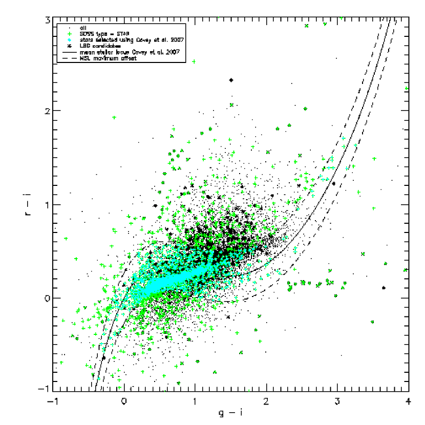
Figure 2: Color-color diagram showing the location of the mean stellar locus (MSL, red solid line) as defined by Covey et al. (2007). The blue dashed lines show the maximum offset to the analytical solution. Point sources within the maximum offset to the MSL are considered stars (cyan dots, making the streak below the MSL). Point sources outside the maximum offset to the MSL are selected as galaxy candidates (green dots). The red stars indicate the location of our LBG candidate sample.

Figure 4: Comparison of the distribution in magnitudes for real (dashed) and simulated (solid) NUV GALEX data. The distributions are consistent with each other. Poisson errors in the real data are omitted for clarity. See text for simulation details.

Figure 7: Total NUV magnitude in relation to the photometric redshift accuracy $\Delta z$. The dashed lines represent the 3$\sigma$ deviation from the $\Delta z$ = 0 line. For galaxies fainter than 23.5 mag, the photometric redshift accuracy decreases significantly.

Figure 9: Distribution of absolute NUV magnitudes (rest frame FUV) used to select the bright and faint LBG subsample. The selection limits are indicated by the values for the M${}^{*}_{NUV}$ of Arnouts et al. (2005, M${}^{*}_{NUV}$ = -19.6, -19.8, -20.0, and -20.2 from low to high redshift) at the individual redshifts.

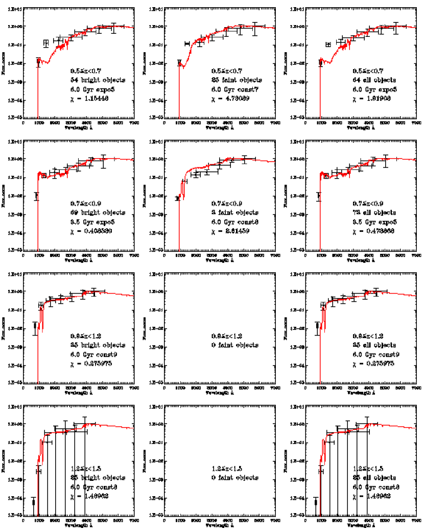
Figure 10a: Averaged spectral energy distribution of the LBG candidates (black) found in the GALEX data. The LBG candidates are fitted with PEGASE models without dust. The samples are divided into bright (left column) and faint (middle column) subsample. The right column shows the results for the combined sample. We also divided the LBG sample into 4 redshift bins from $z\geq$ 0.5 (top) to $z<$ 1.5 (bottom). The green/light lines represent the best fitting model SEDs.

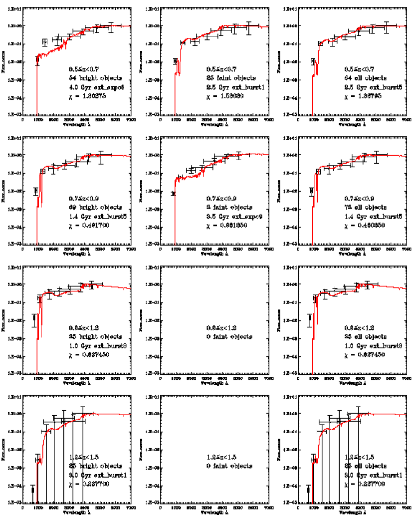
Figure 10b: The same as Fig. 10a, except the inclusion of dust in the PEGASE models. Samples are again divided into bright (left column) and faint (middle column) subsamples. The right column shows the results for the combined samples. From top to bottom we have again plotted the results for the different redshift bins.

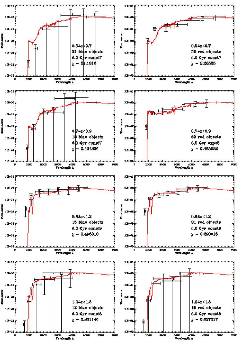
Figure 10c: The diagram shows the result for the SED fitting for blue (left column) and red (right column) subsamples selected using the MSL as defined by Covey et al. (2007, see Fig. 2). The green lines represent the best fitting dust-free model SEDs. We again divided the sample into four subsamples according to the redshift bins from low (top) to high (bottom) redshift.

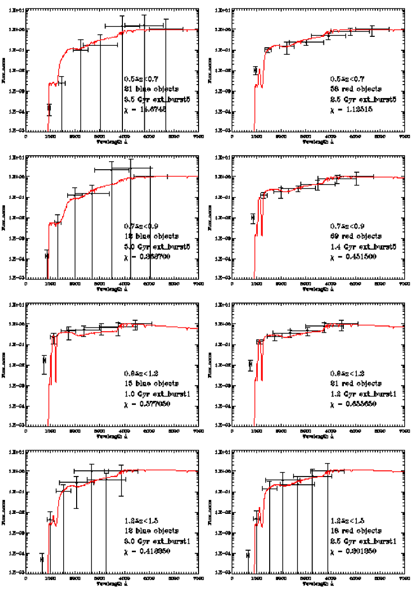
Figure 10d: The same as Fig. 10c, except the inclusion of dust in the PEGASE models.

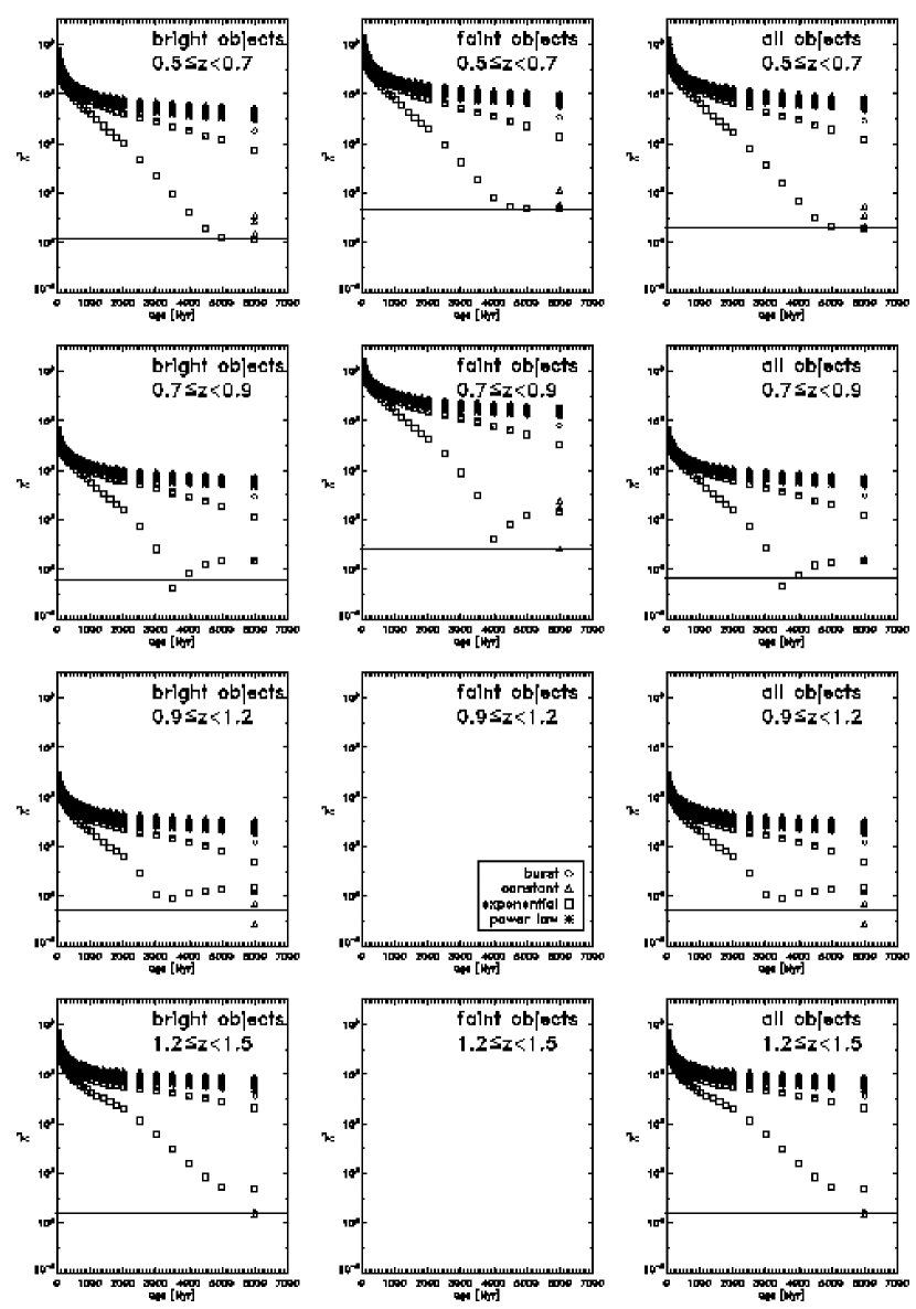
Figure 11a: Results of the model fitting (see Fig. 10a) indicated by the reduced $\chi^{2}$ vs. age in Myr for bright and faint subsamples as well as the complete galaxy sample according to their redshift intervals. The different symbols indicate fit results for different star formation models used (burst: diamonds; constant: triangles; exponential: squares; power law: asterisks). The horizontal lines represent the 1$\sigma$ limits in $\chi^{2}$ for the SED fits.

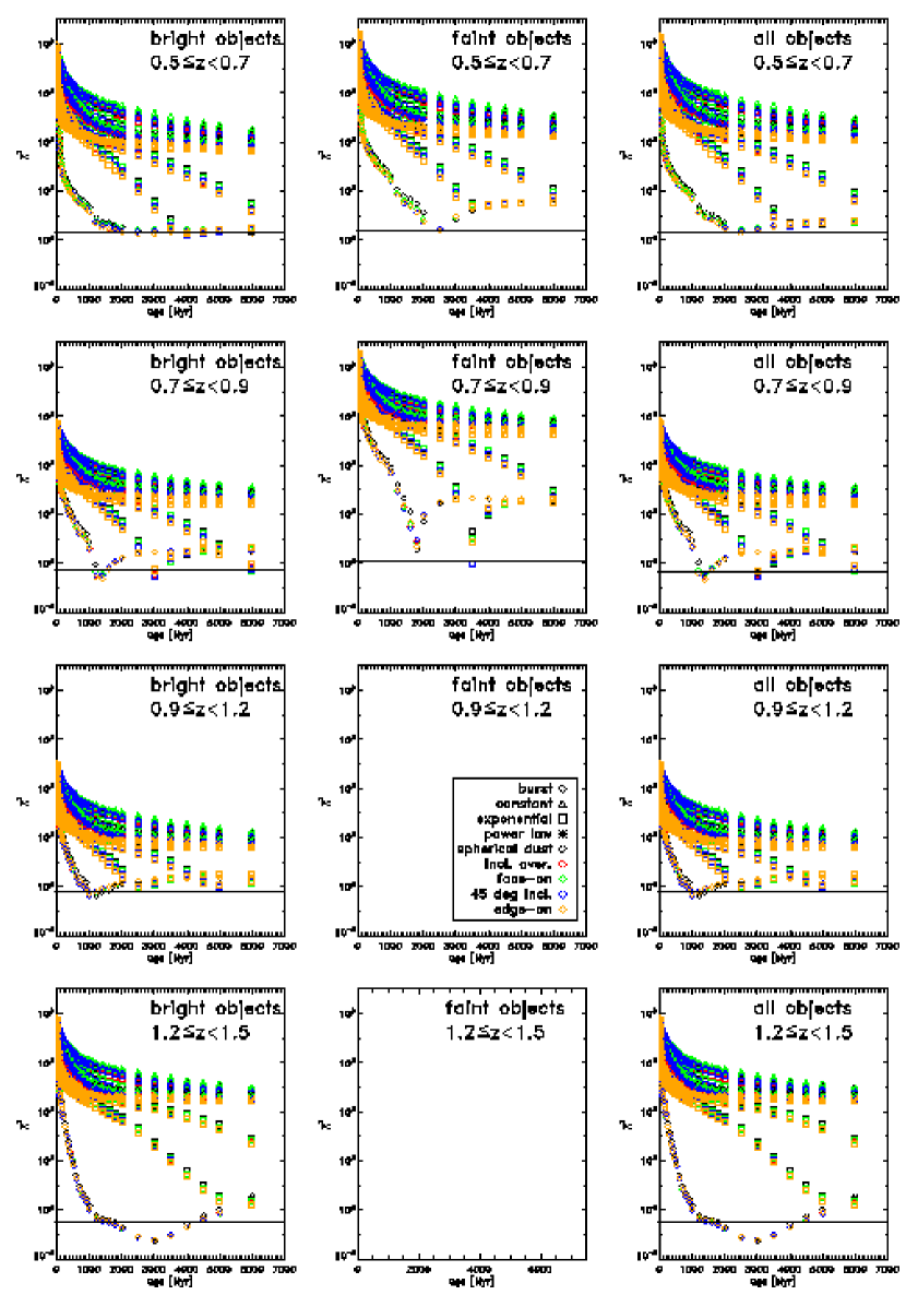
Figure 11b: The same as Fig. 11a, except the inclusion of dust in the PEGASE models. Again different symbols represent different star formation models (burst: diamonds; constant: triangles; exponential: squares; power law: asterisks), while the different colors indicate the use of different dust geometries (spherical: black; disk geometry: inclination averaged – red; face-on – green; 45^∘ – blue; edge-on – orange). The solid lines again represent the $1\sigma$ limits for SED fits (see Fig. 10b).

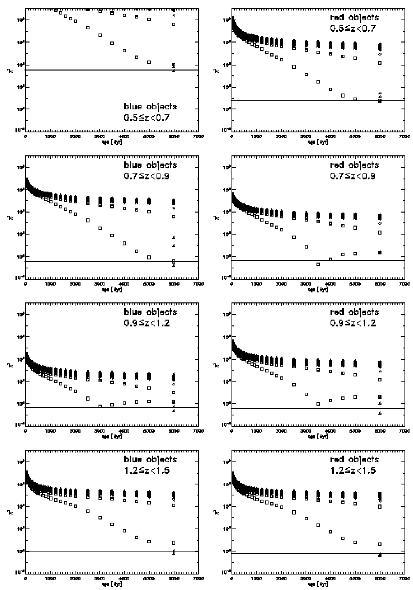
Figure 11c: Results for the SED model fits of the blue and red subsamples (see Fig. 10c). The use of symbols is the same as in Fig. 11a.

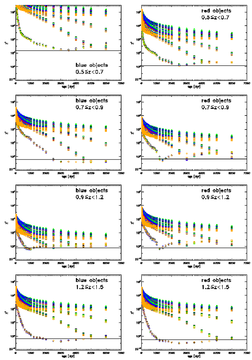
Figure 11d: The same as Fig. 11c, except for the inclusion of dust in the PEGASE models (see Fig. 10d). The notation of symbols and colors is identical to Fig. 11b.

Table 1: Observation summary

	FUV		NUV
Field ID	Texp	mlim	Texp	mlim	Note
	[sec]	[mag]	[sec]	[mag]
(1)	(2)	(3)	(4)	(5)	(6)
21240-GI1_035001_J104802p052610	22902	24	38624	24.0	northern GALEX field
21241-GI1_035002_J105002p042644	20817	24	33021	24.0	southern GALEX field

Note. — The total magnitudes in columns (3) and (5) are the 80 % completeness limits.

Table 2: Examples for LBG candidates

Id	RA(J2000)	DEC(J2000)	FUV	$\Delta$FUV	NUV	$\Delta$NUV	u	$\Delta$u	g	$\Delta$g	r	$\Delta$r	i	$\Delta$i	z	$\Delta$z	$z$	$\Delta$$z$
(1)	(2)	(3)	(4)	(5)	(6)	(7)	(8)	(9)	(10)	(11)	(12)	(13)	(14)	(15)	(16)	(17)	(18)	(19)
LQG_J104745+45136	10:47:45.93	4:51:36.82	25.601	0.855	23.391	0.035	21.880	0.240	21.409	0.061	20.294	0.032	19.807	0.031	19.520	0.104	0.576	0.034
LQG_J104832+45217	10:48:32.36	4:52:17.21	25.732	1.173	23.064	0.032	22.197	0.330	22.282	0.137	21.765	0.126	21.230	0.114	20.961	0.397	0.663	0.220
LQG_J104808+45223	10:48:08.49	4:52:23.37	99.000	99.000	23.314	0.033	22.776	0.446	22.416	0.123	22.119	0.128	21.479	0.106	20.846	0.269	1.154	0.285
LQG_J104710+45329	10:47:10.68	4:53:29.16	25.419	0.779	23.382	0.037	22.420	0.287	22.588	0.121	22.060	0.102	21.911	0.125	21.632	0.428	0.348	0.262
LQG_J104726+45345	10:47:26.29	4:53:45.69	23.411	0.249	20.791	0.007	18.902	0.021	17.756	0.006	17.321	0.005	17.265	0.006	17.222	0.014	0.098	0.015
LQG_J104850+45451	10:48:50.52	4:54:51.50	22.527	0.132	19.450	0.002	15.523	0.009	15.270	0.012	14.503	0.010	11.138	0.001	11.324	0.002	0.851	0.008
LQG_J104656+45529	10:46:56.13	4:55:29.04	22.913	0.184	18.293	0.001	15.433	0.010	11.975	0.001	14.659	0.011	11.102	0.000	13.599	0.016	1.196	0.047
LQG_J104718+45617	10:47:18.30	4:56:17.15	24.271	0.390	20.171	0.003	16.387	0.006	15.045	0.003	14.554	0.004	17.364	0.017	14.330	0.004	1.929	0.004
LQG_J104829+45618	10:48:29.77	4:56:18.67	31.161	180.875	23.206	0.037	22.094	0.782	22.418	0.398	21.160	0.191	19.959	0.096	19.977	0.443	0.798	0.098
LQG_J104735+45712	10:47:35.17	4:57:12.04	25.674	0.956	23.360	0.036	24.247	1.215	22.643	0.159	22.091	0.134	21.638	0.134	20.858	0.289	1.021	0.427
LQG_J104754+45745	10:47:54.93	4:57:45.61	23.499	0.211	20.416	0.004	16.573	0.006	15.109	0.004	14.609	0.004	14.882	0.003	14.420	0.005	0.055	0.032
LQG_J104754+45804	10:47:54.08	4:58:04.16	24.854	0.534	22.771	0.025	22.448	0.428	21.809	0.093	20.712	0.052	20.413	0.057	20.380	0.241	0.416	0.090
LQG_J104851+45808	10:48:51.81	4:58:08.03	24.400	0.498	20.785	0.006	16.396	0.006	14.694	0.004	14.067	0.004	14.119	0.001	13.726	0.004	0.050	0.029
LQG_J104738+45837	10:47:38.29	4:58:37.40	25.209	0.710	23.183	0.034	24.097	1.460	22.021	0.113	21.498	0.109	20.933	0.091	20.573	0.297	0.647	0.106
LQG_J104839+45850	10:48:39.31	4:58:50.02	25.045	0.519	22.835	0.021	22.360	0.282	22.253	0.097	21.842	0.094	21.614	0.112	21.025	0.285	0.553	0.198

Note. — Summary of LBG properties. column (2): RA in hh:mm:ss.ss; column (3) DEC in +dd:mm:ss.ss; column (4) - (17): magnitudes and errors of our 7 band photometry; column (18)+(19): photometric redshifts and errors derived using Hyperz

The complete version of this table is in the electronic edition of the Journal. The printed edition contains only a sample.

Table 3: Summary of selected subsamples

name	$z$	size	FUV	NUV	u	g	r	i	z	FUV-NUV	u-g	g-r	i-z
(1)	(2)	(3)	(4)	(5)	(6)	(7)	(8)	(9)	(10)	(11)	(12)	(13)	(14)
FG1	0.5$\leq$z$<$0.7	64	25.72$\pm$0.60	23.22$\pm$0.23	22.89$\pm$0.52	22.28$\pm$0.35	21.54$\pm$0.48	21.07$\pm$0.58	20.84$\pm$0.68	2.50	0.61	0.74	0.23
LQG0.8	0.7$\leq$z$<$0.9	73	25.97$\pm$1.07	23.08$\pm$0.29	22.69$\pm$0.60	22.27$\pm$0.45	21.77$\pm$0.59	21.05$\pm$0.55	20.90$\pm$0.76	2.90	0.42	0.50	0.15
FG2	0.9$\leq$z$<$1.2	35	25.94$\pm$0.78	23.08$\pm$0.42	22.40$\pm$0.68	22.04$\pm$0.47	21.80$\pm$0.51	21.45$\pm$0.57	21.08$\pm$0.50	2.86	0.35	0.25	0.38
CCLQG	1.2$\leq$z$<$1.5	25	26.16$\pm$1.75	22.07$\pm$1.27	19.48$\pm$2.70	18.86$\pm$3.25	18.72$\pm$3.34	18.54$\pm$3.25	17.83$\pm$3.42	4.08	0.63	0.14	0.72

Note. — The subsamples are selected for the two foreground regions (FG1+FG2) and in the LQGs (LQG0.8+CCLQG). Column (2) gives the redshift interval over which the subsamples were averaged. Columns (4)-(10) present the averaged total magnitudes in the FUV+NUV and 5 SDSS filter bands and columns (11)-(14) summarize the averaged colors for the four subsamples.

Table 4: SED fitting results for bright-faint subsamples

name	redshift	bright		faint		all
	z	best	SFLaw	best	SFLaw	best	SFLaw
		[Gyr]		[Gyr]		[Gyr]
(1)	(2)	(3)	(4)	(5)	(6)	(7)	(8)
FG1	0.5$\leq$z$<$0.7	6.0	expo. decr.	6.0	constant	6.0	expo. decr.
LGQ0.8	0.7$\leq$z$<$0.9	3.5	expo. decr.	6.0	constant	3.5	expo. decr.
FG2	0.9$\leq$z$<$1.2	6.0	constant	$\cdots$	$\cdots$	6.0	constant
CCLQG	1.2$\leq$z$<$1.5	6.0	constant	$\cdots$	$\cdots$	6.0	constant

Note. — Results for the SED fits of the LBG subsamples in the individual redshift bins using PEGASE models without extinction by dust. The table is split into three blocks for the results of the bright (columns (3)+(4)), faint (columns (5)+(6)) LBG subsample as well as the results for the complete LBG candidate sample (columns (7)+(8)). Every block consists of one column for the age and the SFLaw of the best fitting model. The redshift bin is indicated in column (2).

Table 5: SED fitting results for bright-faint subsamples including extinction

name	redshift	bright			faint			all
	z	best	SFLaw	dust geometry	best	SFLaw	dust geometry	best	SFLaw	dust geometry
		[Gyr]		[Gyr]		[Gyr]
(1)	(2)	(3)	(4)	(5)	(6)	(7)	(8)	(9)	(10)	(11)
FG1	0.5$\leq$z$<$0.7	4.0	expo. decr.	face-on disk	2.5	burst	spherical	2.5	burst	edge-on disk
LGQ0.8	0.7$\leq$z$<$0.9	1.4	burst	edge-on disk	3.5	expo. decr.	45∘ incl. disk	1.4	burst	edge-on disk
FG2	0.9$\leq$z$<$1.2	1.0	burst	face-on disk	$\cdots$	$\cdots$	$\cdots$	1.0	burst	face-on disk
CCLQG	1.2$\leq$z$<$1.5	3.0	burst	spherical	$\cdots$	$\cdots$	$\cdots$	3.0	burst	spherical

Note. — Results for the SED fitting of the LBG subsamples for the individual redshift bins as described in Table 4 except now including extinction due to dust in the PEGASE models.

Table 6: SED fitting results for color selected LBG subsamples

name	redshift	blue		red
	z	best	SFLaw	best	SFLaw
		[Gyr]		[Gyr]
(1)	(2)	(3)	(4)	(5)	(6)
FG1	0.5$\leq$z$<$0.7	6.0	constant	6.0	constant
LGQ0.8	0.7$\leq$z$<$0.9	6.0	constant	3.5	expo. decr.
FG2	0.9$\leq$z$<$1.2	6.0	constant	6.0	constant
CCLQG	1.2$\leq$z$<$1.5	6.0	constant	6.0	constant

Note. — Results for the SED fitting of the LBG color selected subsamples using models without extinction by dust. The selection was done according to their location in the g-i vs. r-i color-color diagram. The MSL has been used to separate the blue and red subsample. The table is split into two blocks for the results of the blue (columns (3)+(4)), and red (columns (5)+(6)) LBG subsample. Every block consists of one column for the age and the SFLaw of the best fitting model. The redshift bin is indicated in column (2).

Table 7: SED fitting results for color selected LBG subsamples including extinction

name	redshift	blue			red
	z	best	SFLaw	dust geometry	best	SFLaw	dust geometry
		[Gyr]			[Gyr]
(1)	(2)	(3)	(4)	(5)	(6)	(7)	(8)
FG1	0.5$\leq$z$<$0.7	3.5	burst	face-on disk	2.5	burst	face-on disk
LGQ0.8	0.7$\leq$z$<$0.9	5.0	burst	face-on disk	1.4	burst	face-on
FG2	0.9$\leq$z$<$1.2	1.0	burst	spherical	1.2	burst	spherical
CCLQG	1.2$\leq$z$<$1.5	3.0	burst	spherical	2.5	burst	spherical

Note. — Results for the SED fitting of the LBG subsamples as described in Table 6 now including extinction due to dust in the model SEDs.

References

- Adelberger & Steidel (2005) Adelberger, K. L. & Steidel, C. C. 2005, ApJ, 627, L1
- Adelman-McCarthy et al. (2007) Adelman-McCarthy, J. K., Agüeros, M. A., Allam, S. S., et al. 2007, ApJS, 172, 634
- Adelman-McCarthy et al. (2006) Adelman-McCarthy, J. K., Agüeros, M. A., Allam, S. S., et al. 2006, ApJS, 162, 38
- Arnouts et al. (2005) Arnouts, S., Schiminovich, D., Ilbert, O., et al. 2005, ApJ, 619, L43
- Balogh et al. (2004) Balogh, M. L., Baldry, I. K., Nichol, R., et al. 2004, ApJ, 615, L101
- Bell et al. (2005) Bell, E. F., Papovich, C., Wolf, C., et al. 2005, ApJ, 625, 23
- Bertin & Arnouts (1996) Bertin, E. & Arnouts, S. 1996, A&AS, 117, 393
- Bertin & Fouqué (2007) Bertin, E. & Fouqué, P. 2007, http://terapix.iap.fr
- Bianchi et al. (2007) Bianchi, L., Rodriguez-Merino, L., Viton, M., et al. 2007, ApJS, 173, 659
- Blanton et al. (2003) Blanton, M. R., Brinkmann, J., Csabai, I., et al. 2003, AJ, 125, 2348
- Bolzonella et al. (2000) Bolzonella, M., Miralles, J.-M., & Pelló, R. 2000, A&A, 363, 476
- Bruzual & Charlot (2003) Bruzual, G. & Charlot, S. 2003, MNRAS, 344, 1000
- Burgarella et al. (2007) Burgarella, D., Le Floc’h, E., Takeuchi, T. T., et al. 2007, MNRAS, 380, 986
- Burgarella et al. (2006) Burgarella, D., Pérez-González, P. G., Tyler, K. D., et al. 2006, A&A, 450, 69
- Cassata et al. (2007) Cassata, P., Guzzo, L., Franceschini, A., et al. 2007, ApJS, 172, 270
- Clowes & Campusano (1991) Clowes, R. G. & Campusano, L. E. 1991, MNRAS, 249, 218
- Clowes & Campusano (1994) Clowes, R. G. & Campusano, L. E. 1994, MNRAS, 266, 317
- Clowes et al. (1999) Clowes, R. G., Campusano, L. E., & Graham, M. J. 1999, MNRAS, 309, 48
- Coia et al. (2005) Coia, D., Metcalfe, L., McBreen, B., et al. 2005, A&A, 430, 59
- Cooper et al. (2007) Cooper, M. C., Newman, J. A., Weiner, B. J., et al. 2007, MNRAS, 1119
- Cooper et al. (2008) Cooper, M. C., Newman, J. A., Weiner, B. J., et al. 2008, MNRAS, 383, 1058
- Covey et al. (2007) Covey, K. R., Ivezić, Ž., Schlegel, D., et al. 2007, AJ, 134, 2398
- Croom et al. (2004) Croom, S. M., Smith, R. J., Boyle, B. J., et al. 2004, MNRAS, 349, 1397
- D’Odorico et al. (2008) D’Odorico, V., Bruscoli, M., Saitta, F., et al. 2008, MNRAS, 389, 1727
- Doroshkevich & Dubrovich (2001) Doroshkevich, A. & Dubrovich, V. 2001, MNRAS, 328, 79
- Duc et al. (2002) Duc, P.-A., Poggianti, B. M., Fadda, D., et al. 2002, A&A, 382, 60
- Eales (1993) Eales, S. 1993, ApJ, 404, 51
- Elbaz et al. (2007) Elbaz, D., Daddi, E., Le Borgne, D., et al. 2007, A&A, 468, 33
- Ellis et al. (1996) Ellis, R. S., Colless, M., Broadhurst, T., Heyl, J., & Glazebrook, K. 1996, MNRAS, 280, 235
- Evrard et al. (2002) Evrard, A. E., MacFarland, T. J., Couchman, H. M. P., et al. 2002, ApJ, 573, 7
- Fioc & Rocca-Volmerange (1997) Fioc, M. & Rocca-Volmerange, B. 1997, A&A, 326, 950
- Foucaud et al. (2003) Foucaud, S., McCracken, H. J., Le Fèvre, O., et al. 2003, A&A, 409, 835
- Gerke et al. (2007) Gerke, B. F., Newman, J. A., Faber, S. M., et al. 2007, MNRAS, 376, 1425
- Graham et al. (1995) Graham, M. J., Clowes, R. G., & Campusano, L. E. 1995, MNRAS, 275, 790
- Guillemin & Bergeron (1997) Guillemin, P. & Bergeron, J. 1997, A&A, 328, 499
- Haberzettl et al. (2009) Haberzettl, L., Bomans, D. J., & Dettmar, R.-J. 2009, A&A in prep.
- Haberzettl et al. (2009) Haberzettl et al. 2009, in prep.
- Haines et al. (2004) Haines, C. P., Campusano, L. E., & Clowes, R. G. 2004, A&A, 421, 157
- Haines et al. (2001) Haines, C. P., Clowes, R. G., Campusano, L. E., & Adamson, A. J. 2001, MNRAS, 323, 688
- Haines et al. (2007) Haines, C. P., Gargiulo, A., La Barbera, F., et al. 2007, MNRAS, 381, 7
- Harris et al. (2009) Harris et al. 2009, in prep.
- Hildebrandt et al. (2007) Hildebrandt, H., Pielorz, J., Erben, T., et al. 2007, A&A, 462, 865
- Hogg (1999) Hogg, D. W. 1999, ArXiv Astrophysics e-prints astro-ph/9905116
- Hogg (2001) Hogg, D. W. 2001, AJ, 121, 1207
- Hopkins et al. (2008) Hopkins, P. F., Hernquist, L., Cox, T. J., & Kereš, D. 2008, ApJS, 175, 356
- Kocevski et al. (2008a) Kocevski, D. D., Lubin, L. M., Gal, R., et al. 2008a, ArXiv e-prints, 804
- Kocevski et al. (2008b) Kocevski, D. D., Lubin, L. M., Lemaux, B. C., et al. 2008b, ArXiv e-prints, 809
- Koyama et al. (2008) Koyama, Y., Kodama, T., Shimasaku, K., et al. 2008, MNRAS, 391, 1758
- Lilly et al. (1995) Lilly, S. J., Tresse, L., Hammer, F., Crampton, D., & Le Fevre, O. 1995, ApJ, 455, 108
- Madau et al. (1998) Madau, P., Pozzetti, L., & Dickinson, M. 1998, ApJ, 498, 106
- Marmo & Bertin (2008) Marmo, C. & Bertin, E. 2008, in Astronomical Society of the Pacific Conference Series, Vol. 394, Astronomical Data Analysis Software and Systems XVII, ed. R. W. Argyle, P. S. Bunclark, & J. R. Lewis, 619+–
- Massarotti et al. (2001) Massarotti, M., Iovino, A., Buzzoni, A., & Valls-Gabaud, D. 2001, A&A, 380, 425
- Nagamine (2002) Nagamine, K. 2002, ApJ, 564, 73
- Nagamine et al. (2000) Nagamine, K., Cen, R., & Ostriker, J. P. 2000, ApJ, 541, 25
- Nakata et al. (2002) Nakata, F., Kodama, T., Shimasaku, K., et al. 2002, in 8th Asian-Pacific Regional Meeting, Volume II, ed. S. Ikeuchi, J. Hearnshaw, & T. Hanawa, 283–284
- Newman (1999) Newman, P. R. 1999, PhD thesis, AA(University of Central Lancashire prnewman@uclan.ac.uk)
- Noeske et al. (2007) Noeske, K. G., Weiner, B. J., Faber, S. M., et al. 2007, ApJ, 660, L43
- Papovich et al. (2001) Papovich, C., Dickinson, M., & Ferguson, H. C. 2001, ApJ, 559, 620
- Peng et al. (2002) Peng, C. Y., Ho, L. C., Impey, C. D., & Rix, H.-W. 2002, AJ, 124, 266
- Pettini et al. (2001) Pettini, M., Shapley, A. E., Steidel, C. C., et al. 2001, ApJ, 554, 981
- Pilipenko (2007) Pilipenko, S. V. 2007, Astronomy Reports, 51, 820
- Porciani & Giavalisco (2002) Porciani, C. & Giavalisco, M. 2002, ApJ, 565, 24
- Porter et al. (2008) Porter, S. C., Raychaudhury, S., Pimbblet, K. A., & Drinkwater, M. J. 2008, MNRAS, 388, 1152
- Postman et al. (2005) Postman, M., Franx, M., Cross, N. J. G., et al. 2005, ApJ, 623, 721
- Quadri et al. (2007) Quadri, R., van Dokkum, P., Gawiser, E., et al. 2007, ApJ, 654, 138
- Richards et al. (2007) Richards, G. T., Myers, A., Brunner, R., et al. 2007, in Bulletin of the American Astronomical Society, Vol. 38, Bulletin of the American Astronomical Society, 994+–
- Sawicki & Thompson (2006) Sawicki, M. & Thompson, D. 2006, ApJ, 648, 299
- Schmidt (1968) Schmidt, M. 1968, ApJ, 151, 393
- Schneider et al. (2007) Schneider, D. P., Hall, P. B., Richards, G. T., et al. 2007, AJ, 134, 102
- Silverman (1986) Silverman, B. W. 1986, Density estimation for statistics and data analysis (Monographs on Statistics and Applied Probability, London: Chapman and Hall, 1986)
- Söchting et al. (2002) Söchting, I. K., Clowes, R. G., & Campusano, L. E. 2002, MNRAS, 331, 569
- Söchting et al. (2004) Söchting, I. K., Clowes, R. G., & Campusano, L. E. 2004, MNRAS, 347, 1241
- Steidel et al. (1997) Steidel, C. C., Dickinson, M., Meyer, D. M., Adelberger, K. L., & Sembach, K. R. 1997, ApJ, 480, 568
- Steidel et al. (1996) Steidel, C. C., Giavalisco, M., Pettini, M., Dickinson, M., & Adelberger, K. L. 1996, ApJ, 462, L17+
- Steidel et al. (1995) Steidel, C. C., Pettini, M., & Hamilton, D. 1995, AJ, 110, 2519
- Swinbank et al. (2007) Swinbank, A. M., Edge, A. C., Smail, I., et al. 2007, MNRAS, 379, 1343
- Teplitz et al. (2000) Teplitz, H. I., McLean, I. S., Becklin, E. E., et al. 2000, ApJ, 533, L65
- Vijh et al. (2003) Vijh, U. P., Witt, A. N., & Gordon, K. D. 2003, ApJ, 587, 533
- Williger et al. (2002) Williger, G. M., Campusano, L. E., Clowes, R. G., & Graham, M. J. 2002, ApJ, 578, 708
- Willmer et al. (2006) Willmer, C. N. A., Faber, S. M., Koo, D. C., et al. 2006, ApJ, 647, 853
- Wolf et al. (2005) Wolf, C., Bell, E. F., McIntosh, D. H., et al. 2005, ApJ, 630, 771