Galaxy cluster mergers

Abstract

We present the results of an Eulerian adaptive mesh refinement (AMR) hydrodynamical and N-body simulation in a $\Lambda$CDM cosmology. The simulation incorporates common cooling and heating processes for primordial gas. A specific halo finder has been designed and applied in order to extract a sample of galaxy clusters directly obtained from the simulation without considering any resimulating scheme. We have studied the evolutionary history of the cluster halos, and classified them into three categories depending on the merger events they have undergone: major mergers, minor mergers, and relaxed clusters. The main properties of each one of these classes and the differences among them are discussed. The collisions among galaxy clusters are produced naturally by the non-linear evolution in the simulated cosmological volume, no controlled collisions have been considered. We pay special attention to discuss the role of merger events as a source of feedback and reheating, and their effects on the existence of cool cores in galaxy clusters, as well as in the scaling relations.

1 Introduction

Galaxy clusters are crucial pieces in our understanding of the Universe. They represent the transition between two different regimes. The first one involves the evolution of perturbations on cosmological scales where the physics of the problem is only driven by gravity on the dark matter component. The second one, is the scenario of galactic scales, where the action of gravity is combined with the effects of a complex gas dynamics and all sort of astrophysical phenomena (cooling, star formation, feedback, …).

Precisely, due to its nature linking different scales, the galaxy clusters provide us with a powerful tool to constrain the cosmological parameters, and at the same time, they help us to understand the physical properties of the intra-cluster medium (ICM) and its interplay with galaxy formation and evolution. In this sense, galaxy clusters are extremely valuable laboratories where explore the connection between cosmological scales and the formation and evolution of galaxies.

The simplest model explaining the properties of the ICM  (Kaiser, 1986) assumes that gravity is the only responsible force determining the evolution of the ICM. In this scenario, the gas collapses into the dark matter potential wells and then, accretion shocks form moving outwards in the cluster and heating up the gas until the virial temperature of the halo  (Quilis, Ibáñez & Sáez, 1998). As gravity acts on all scales, this model has been known as self-similar.

This model gives us precise predictions for the properties of galaxy clusters: X-ray luminosity, temperature, entropy, and mass  (Bryan & Norman, 1998). However, the scaling relations produced by the self-similar model do not match the observational results completely. More specifically, the slope of the X-ray luminosity-temperature relation is steeper than predicted  (Markevitch, 1998; Arnaud & Evrard, 1999; Osmond & Ponman, 2004), the measured gas entropy in poor clusters and groups is higher than expected  (Ponman, Sanderson & Finoguenov, 2003), and it has been observed a decreasing trend of the gas mass fraction in poorer systems  (Balogh et al., 2001; Lin, Mohr & Stanford, 2003; Sanderson et al., 2003). In addition, there is an important scatter in the relations  (Fabian et al., 1994) partly, but not totally, connected with the effect of the different environments where clusters live.

Those discrepancies between the self-similar model and the observations have motivated the idea that some important physics, basically related with the baryonic component, is missing in the model.

Some of these non-gravitational processes have been included in simulations trying to solve the similarity breaking: preheating  (Navarro, Frenk & White, 1995; Bialek, Evrard & Mohr, 2001; Borgani et al., 2002), and radiative cooling  (Pearce et al., 2000; Muanwong et al., 2001; Davé, Katz & Weinberg, 2002; Molt et al., 2004; Kravtsov, Nagai & Vikhlinin, 2005). More sophisticated approaches coupling the feedback with cooling and star formation have been carried out by Kay, Thomas & Theuns (2003); Tornatore et al. (2003); Valdarnini (2003); Borgani et al. (2004); Ettori et al. (2004); Kay et al. (2004, 2007) among others.

Merger events can also be an important source of feedback in galaxy clusters. They can produce shocks and compression waves in the halos which eventually can release part of the energy associated with the collision as thermal energy in the final system  (McCarthy et al., 2007). It is likely that turbulence and mixing could play an important role in how this energy is mixed and released in the ICM of the final halo after the merger. As it is well known, some of the results of these simulations could depend on the ability of different numerical techniques to describe shock waves, strong gradients, turbulence, and mixing, which can be very different. Although is still a matter of debate, it has been shown, at least for some idealised tests, that the comparison between grid codes and SPH codes – when numerical resolution is similar – can give substantial differences in the results  (Frenk et al., 1999; Agertz et al., 2007). It seems reasonable to think that these inherent numerical differences could translate into relevant differences when they are applied to more complex and realistic scenarios like galaxy clusters. This situation makes interesting, and complementary, to pursue the number of studies using the different numerical strategies available.

In this paper, we want to investigate the role of the galaxy cluster mergers as a source of feedback and reheating in a complete general cosmological framework. The galaxy clusters form and evolve due to the non-linear evolution of primordial perturbations, and therefore, no special symmetry or idealised clusters are considered. In this scenario, the merger events naturally take place according to the hierarchical evolution. Previous works have extensively studied the mergers of galaxy clusters using controlled collisions (e.g. Ricker & Sarazin (2001); Poole et al. (2006, 2007); McCarthy et al. (2007); Poole et al. (2008)). The approach adopted in the present paper could be considered as complementary to the studies using controlled mergers. It is clear that our approach has some important weaknesses, when it is compared with controlled mergers, like the worst resolution or the impossibility to control the different parameters involved in the problem. However, it gives a description of the problem in a cosmological context, without symmetries, including the presence of substructures and taking into account the effects of the different environments.

In order to study the role of mergers, fulfilling all the previous requirements, we have carried out a simulation of a moderate size box of side length $100\,h^{-1}\,Mpc$. We have performed it with an Eulerian AMR cosmological code including the usual processes of cooling and heating for primordial gas, and a phenomenological star formation treatment. We have identified and followed the evolution of the different galaxy cluster halos. Once the evolutionary history of the halos is known, we have classified them into three broad categories depending on the features of the merger events in which they have been involved. We will discuss their effects on cluster properties. These mergers are the ones naturally happening in the building up of the galaxy clusters.

The paper is organized as follows. In Section 2, we present the details of the simulation and describe the halo finder used to identify the galaxy cluster halos. In Section 3, we analyse the results of the simulation describing the main properties of the galaxy cluster sample, and the effects of mergers. Finally, in Section 4, we summarise and discuss our results.

Table 1: Cluster sample. Main features of selected clusters at $z=0$. Column 2, virial radius in units of $h^{-1}\,Mpc$; column 3, total mass within the virial radius in units of $10^{14}\,M_{\odot}$; column 4, mass-weighted temperature within the virial radius in $keV$; column 5, gaseous mass within the virial radius in units of $10^{14}\,M_{\odot}$; column 6, average entropy within the virial radius in units of $keVcm^{2}$; column 7, type classification: relaxed or with no important mergers (R), minor mergers (MI), and major mergers (MA).

cluster	$r_{vir}$	$M_{vir}$	T	$m_{gas}$	$S$	type
	$(h^{-1}\,Mpc)$	$(10^{14}\,M_{\odot})$	$(keV)$	$(10^{14}\,M_{\odot})$	$(keVcm^{2})$
CL01	2.32	18.61	7.02	3.45	2601.06	MA
CL02	2.22	15.83	5.99	4.89	2130.17	MA
CL03	1.58	5.68	3.24	1.08	919.34	MA
CL04	1.48	4.70	3.80	0.79	998.65	MA
CL05	1.39	3.93	2.29	0.70	1063.19	MA
CL06	1.07	1.86	1.26	0.37	510.01	MA
CL07	1.01	1.53	1.01	0.25	846.33	MA
CL08	0.93	1.14	0.87	0.21	422.39	MA
CL09	1.51	5.19	3.09	1.03	1166.28	MI
CL10	1.51	5.11	2.18	0.92	1126.22	MI
CL11	1.36	3.76	2.55	0.49	862.07	MI
CL12	1.45	4.40	2.52	0.97	980.39	R
CL13	1.10	1.99	1.40	0.41	409.21	R
CL14	0.99	1.39	1.18	0.29	362.36	R
CL15	0.89	1.02	0.97	0.22	554.70	R
CL16	0.89	1.01	0.90	0.22	386.56	R

2 The simulation

2.1 Simulation details

The simulation described in this paper has been performed with the cosmological code MASCLET (Quilis, 2004). This code couples an Eulerian approach based on high-resolution shock capturing techniques for describing the gaseous component, with a multigrid particle mesh N-body scheme for evolving the collisionless component (dark matter). Gas and dark matter are coupled by the gravity solver. Both schemes benefit of using an adaptive mesh refinement (AMR) strategy, which permits to gain spatial and temporal resolution.

The numerical simulation has been performed assuming a spatially flat $\Lambda CDM$ cosmology, with the following cosmological parameters: matter density parameter, $\Omega_{m}=0.25$; cosmological constant, $\Omega_{\Lambda}=\Lambda/{3H_{o}^{2}}=0.75$; baryon density parameter, $\Omega_{b}=0.045$; reduced Hubble constant, $h=H_{o}/100km\,s^{-1}\,Mpc^{-1}=0.73$; power spectrum index, $n_{s}=1$; and power spectrum normalisation, $\sigma_{8}=0.8$.

The initial conditions were set up at $z=50$, using a CDM transfer function from Eisenstein & Hu (1998), for a cube of comoving side length $100\,h^{-1}\,Mpc$. The computational domain was discretized with $512^{3}$ cubical cells.

A first level of refinement (level 1) for the AMR scheme was set up from the initial conditions by selecting regions satisfying certain refining criteria, when evolved – until present time – using the Zeldovich approximation. The volumes selected as refinable were covered by grids (patches) with numerical cells selected from the initial conditions. The regions of the box not eligible to be refined were degraded in resolution by averaging the quantities obtained on the initial grid. This procedure creates the coarse grid (level 0) for the AMR scheme. These coarse cells have a volume eight times larger than the first level ones. In the same manner, the dark matter component within the refined regions was sampled with dark matter particles eight times lighter than those used in regions covered only by the coarse grid. During the evolution, regions on the different grids are refined based on the local baryonic and dark matter densities. Any cell with a baryon mass larger than $5.6\times 10^{8}M_{\odot}$ or a dark matter mass larger than $2.5\times 10^{9}M_{\odot}$ was labelled as refinable. The ratio between the cell sizes for a given level ($l+1$) and its parent level ($l$) is, in our AMR implementation, $\Delta x_{l+1}/\Delta x_{l}=1/2$. This is a compromise value between the gain in resolution and possible numerical instabilities. This method produces patches with a boxy geometry and cubic cells at any level.

The simulation presented in this paper has used a maximum of seven levels ($l=7$) of refinement, which gives a peak spatial resolution of $3\,h^{-1}\,kpc$. For the dark matter we consider two particles species, which correspond to the particles on the coarse grid and the particles within the first level of refinement at the initial conditions. The best mass resolution is $5.75\times 10^{8}\,h^{-1}\,M_{\odot}$, equivalent to distribute $512^{3}$ particles in the whole box.

Our simulation includes cooling and heating processes which take into account Compton and free-free cooling, UV heating (Haardt & Madau, 1996), and atomic and molecular cooling for a primordial gas. In order to compute the abundances of each species, we assume that the gas is optically thin and in ionization equilibrium, but not in thermal equilibrium (Katz, Weinberg & Hernquist, 1996; Theuns et al., 1998). The tabulated cooling rates were taken from Sutherland & Dopita (1993) assuming a constant metallicity 0.3 relative to solar. The cooling curve was truncated below temperatures of $10^{4}\,K$. The cooling and heating were included in the energy equation (see Eq.(3) in Quilis (2004)) as extra source terms.

The star formation has also been modelled with the phenomenological approach commonly used in cosmological simulations (i.e. Yepes et al. (1997); Springel & Hernquist (2003)). A more detailed description of how star formation has been introduced in MASCLET code is presented in Appendix A. Despite the use of an AMR code to perform the simulation described in the present paper, we have still had numerical limitations, namely, the number of patches placed at the highest level of refinement. Although this limitation has been not crucial for the description of clusters, it has translated into a poor star formation efficiency as the analysed run only allowed star formation at the highest level of refinement. This apparent drawback of our simulation is not dramatic for the purpose of the present study where we focus in the effect of mergers on the ICM properties. Thus, the stellar feedback has turned out to be very low, and consequently, it does not alter the pure effect of the mergers.

Figure 1: Merger tree for one cluster of each category: left panel shows a major merger cluster, central panel represents a minor merger cluster, and right panel stands for a relaxed cluster. Cluster halos are represented by circles whose sizes are normalised to the final mass at $z=0$. Lines connecting halos at different times indicate the amount of mass transferred from the progenitors to their descendants.

2.2 Cluster identification

A crucial issue in the analysis of our simulation has to do with the cluster identification. In order to do so, we have developed a halo finding method specially suited for the features of the cosmological code MASCLET.

The halo finder developed for MASCLET code follows a similar idea to MHF halo finder (Gill, Knebe & Gibson, 2004). The main aim is to identify gravitationally bound objects in a N-body simulation.

We have used an identification technique based on the original idea of the spherical over-density (SO) method. The basic concept of this technique is to identify spherical regions with an average density above a certain threshold, which can be fixed according to the spherical top-hat collapse model. Therefore, we can define the viral mass of a halo, $M_{vir}$, as the mass enclosed in a spherical region of radius, $r_{vir}$, having an average density $\Delta_{c}$ times the critical density $\rho_{c}(z)=3H(z)^{2}/8\pi G$:

$$M_{vir}(<r_{vir})=\frac{4}{3}\pi r_{vir}^{3}\Delta_{c}\rho_{c}.$$ (1)

The over-density $\Delta_{c}$ depends on the adopted cosmological model, and can be approximated by the following expression (Bryan & Norman, 1998):

$$\Delta_{c}=18\pi^{2}+82x-39x^{2}$$ (2)

where $x=\Omega(z)-1$ and $\Omega(z)=[\Omega_{m}(1+z)^{3}]/[\Omega_{m}(1+z)^{3}+\Omega_{\Lambda}]$. Typical values of $\Delta_{c}$ are between 100 and 500, in particular, for the cosmological parameters considered in our simulation, $\Delta_{c}\simeq 373$.

The SO method implies oversimplifications which could lead to somehow artificial results which deserve a careful treatment. The enforced spherical symmetry for halos that, at least at some moments of their lives, can have quite irregular structures (e.g.,  White (2002)), or the difficulties to discriminate among close density peaks, are some of these well known problems.

The practical implementation of our halo finder has several steps designed to improve the performance of the SO method and to get rid of the possible drawbacks. In a first step, the algorithm finds halos by centring at density peaks and growing spheres until the average over-density falls below $\Delta_{c}$, or there is a rising up of the slope of the density profile. The second step takes care of possible overlaps among the preliminary halos found in the first step. In our method, halos which overlap more than 30% and less than 80% in mass are joined as a single one. Halos sharing more than 80% of their mass are considered as a misidentification and one of them drops out of the list. The third step checks that all particles contained in a halo are bound. In order to determine whether a particle is bound or not, we estimate the escape velocity at the position of the particle (, 1999). If the velocity of a particle is larger than the escape velocity, the particle is assumed to be unbound. A final step verifies that the density profile is consistent with a NFW profile (Navarro, Frenk & White, 1997).

One of the main advantages of our method is that the structure of nested grids created by the AMR scheme already follows the density peaks, and therefore, densities are already calculated by the cosmological code. Other important point, inherent to the structure of the AMR scheme used, is that no linking length is needed. The process of halo finding can be performed, independently, at each level of refinement of the simulation. Then, in a natural way, our halo finder can trace halos-in-halos and obtain a hierarchy of nested halos.

The different progenitors are identified by following all particles belonging to a given halo backwards in time. This procedure can be repeated until the first progenitor of a certain halo is found. This method allows us, not only to know all the progenitors of each halo, but the amount of mass received from each one of its ancestors.

3 Results

In our simulation, we have identified more than three hundred galaxy clusters and groups spanning a range of masses from $1.0\times 10^{13}\,M_{\odot}$ to $2.0\times 10^{15}\,M_{\odot}$. We refer to this set of clusters as the complete sample. We have constructed their evolutionary histories and, based on their merging histories, we have classified them into three categories according to the mass ratio of the halos involved in the collision.

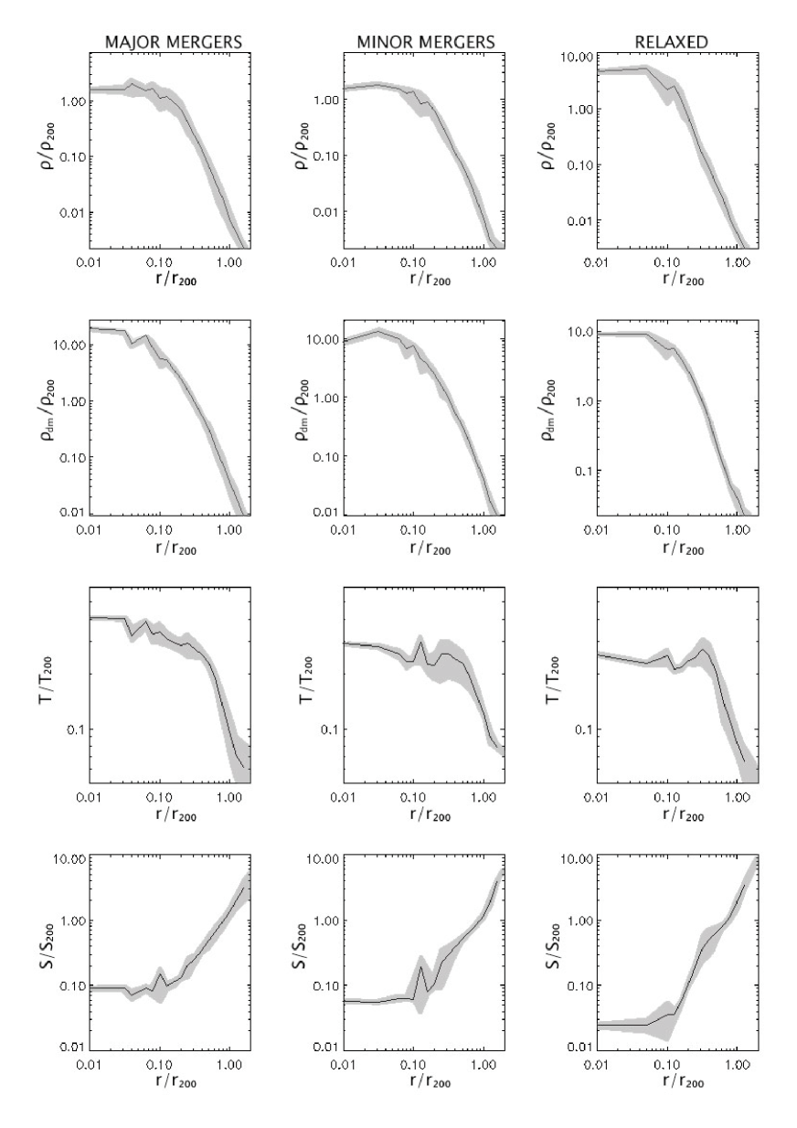
Figure 2: Average radial profiles for all clusters belonging to each class: major mergers (left column), minor mergers (central column), and relaxed (right column). From top to bottom, the first and second rows display gas ($\rho/\rho_{{}_{200}}$) and dark matter ($\rho_{dm}/\rho_{{}_{200}}$) densities, respectively, the third row shows mass-weighted temperature ($T/T_{{}_{200}}$), and the fourth row represents entropy ($S/S_{{}_{200}}$). All profiles have been scaled by the mean value of the plotted quantities within the scale radius, $r_{{}_{200}}$. Continuous lines show the average for all the individual profiles of each class of clusters. Shadowed regions represent one $\sigma$ deviation.

It is also convenient to adopt a timescale limit since mergers occurring at a very early epoch would not have any important consequence on the present properties of the clusters. In this sense, and only for the purpose of delimiting the merger events happening recently, we have defined the formation redshift of a cluster, $z_{for}$, as the redshift at which the cluster mass is half of its present virial mass  (Lacey & Cole, 1993). Thus, we consider for each cluster only those mergers that have relevant effects on its recent past.

Therefore, taking into account the formation redshift of the clusters, $z_{for}$, and the masses of the most (less) massive halo, $m_{2}\,\,(m_{1})$, involved in the merger, we have classified the clusters into three categories:

• Major mergers. Those systems where the mass ratio $m_{2}:m_{1}$ is smaller than $3:1$. Therefore, a major merger involves clusters with similar masses.

• Minor mergers. Those systems where the mass ratio is $3:1<m_{2}:m_{1}<10:1$.

• Relaxed halos. Those systems which have suffered mergers with very small halos, $10:1<m_{2}:m_{1}$, or smooth accretion.

Out of the complete sample, we have picked up a subsample which contains the sixteen most massive galaxy clusters in the computational box. They constitute what it would be referred to as the reduced sample, and their main features are summarised in Table 1. Depending on the particular analysis, that we will be interested in the following sections of this paper, we will use the complete or the reduced sample, respectively. Concerning their merging classification, in the reduced sample we have found five relaxed clusters (R), three have been categorised as clusters with minor mergers (MI), and eight have been classified as major merger systems (MA).

Despite we have used an AMR code to carry out the simulation described in this paper, due to numerical limitations, a biased sample of clusters – with a tendency to better describe the most massive ones – has been produced. These artificial results could be overcome, in future applications, by performing resimulations of the selected clusters in the sample, although this could prevent us from following the mergers in a cosmological context. In any case, we consider that the effects of mergers would be more important in those systems with higher masses – well described in the present simulation – and therefore, we believe that this bias has only minor consequences.

In order to analyse the results of our simulation, we will study several thermodynamical properties which can be directly connected with observational data, and which have been widely studied by all sort of different simulations. In addition to the common plots of density, we will also study the behaviour of the ICM temperature, X-ray luminosity, entropy, and the internal and kinetic energies.

The ICM temperature will be defined as:

$$T=\frac{\sum_{i}T_{i}w_{i}}{\sum_{i}w_{i}},$$ (3)

where $T_{i}$ and $w_{i}$ are the temperature and the weight given to each cell. In most of the applications in the present paper, the weight will be the cell mass, $w_{i}=m_{i}$, and therefore, this will be a mass-weighted temperature. In some particular cases, and for the sake of comparison with observational data, we will also use the so called spectroscopic-like temperature  (Mazzotta et al., 2004), $T_{sl}$, where the weight is $w_{i}=m_{i}\rho_{i}T_{i}^{-3/4}$ with $\rho_{i}$ the density at the cell $i$.

A crucial observable quantity, directly related with the temperature and the density of the gas, is the bolometric X-ray luminosity. In simulations, this quantity can be computed by adding up all the contributions from each elemental volume of gas:

$$L_{{}_{X}}=\int_{V}n_{e}n_{i}\Lambda(T,Z)\,dV$$ (4)

where $n_{e}$ and $n_{i}$ are the electron and ion density, respectively, and $\Lambda$ is the normalised cooling function depending on the temperature (T) and metallicity (Z) from Sutherland & Dopita (1993) (see Sec. 2.1).

The next thermodynamical quantity we will pay a special attention is the entropy, which is an extremely useful quantity providing a lot of information (Voit, 2005) about the evolutionary state of the clusters, since it records the thermodynamical history of the ICM produced by the gravitational and non-gravitational processes. We will adopt the following common definition for the entropy:

$$S=k_{B}Tn_{e}^{-2/3},$$ (5)

where $n_{e}$ is the electron number density and $k_{B}$ is the Boltzmann constant.

Other thermodynamical quantities useful to quantify the effects of mergers and shocks as a source of feedback are the total internal energy, $E_{u}$, and the total kinetic energy, $E_{k}$, which are given by the following expressions:

$$E_{u}=\int_{V_{vir}}\rho\epsilon\,dV$$ (6)

$$E_{k}=\frac{1}{2}\int_{V_{vir}}\rho v^{2}\,dV$$ (7)

where $\rho$, $\epsilon$ and $v$ are the gas density, specific internal energy and the peculiar velocity of the gas fluid element, respectively.

For the sake of comparison with observational data, it is also useful to define some characteristic quantities widely used in the literature. Similar to the definition of the virial quantities (see Sec. 2.2), we introduce a characteristic radius, $r_{{}_{\Delta}}$, such that the mean density enclosed within this radius is $\Delta$ times $\rho_{c}$, and therefore, the mass is:

$$M_{\Delta}(<r_{{}_{\Delta}})=\frac{4}{3}\pi r_{{}_{\Delta}}^{3}\Delta\rho_{c}.$$ (8)

Consequently, we follow the common definition for the temperature,

$$T_{{}_{\Delta}}=\frac{GM_{{}_{\Delta}}}{2r_{{}_{\Delta}}}\frac{\mu m_{p}}{k_{B}},$$ (9)

where $\mu$ and $m_{p}$ are the mean atomic weight and the proton mass. In the same manner, we define the entropy,

$$S_{{}_{\Delta}}=k_{B}T_{{}_{\Delta}}\left(\frac{\mu m_{p}}{f_{b}\rho_{{}_{\Delta}}}\right)^{2/3},$$ (10)

with $f_{b}=\Omega_{b}/\Omega_{m}$.

In the following sections, and in order to compare with previous works, we will consider $\Delta=200$ or $\Delta=500$, depending on the particular case we compare with. All the quantities we have just described, are going to be used to analyse the results of the simulation.

3.1 Merger history of selected clusters

We have constructed the merger tree of the selected galaxy clusters tracking all the dark matter particles that belong to a given cluster backwards in time. Figure 1 displays the merger trees of three halos, which could be considered as prototypical ones of each category (i.e., relaxed, minor merger, and major merger). The clusters have been selected such that they have very similar masses and sizes at $z=0$. The merger trees start at $z=0$ and plot all the parent halos of the final ones in previous time steps over several output times of the simulation.

The total mass of each halo is represented by a circle, whose size is normalised to the mass of the final halo at $z=0$. The lines connecting circles between different times inform us about the progenitors of a given halo at a given time. In addition, the type of line tells us the amount of mass transferred from the progenitor to the halo at the considered time. Thus, a halo at a certain time connected with a progenitor halo at earlier time by a dash-dotted line, means that up to 25% of its mass is due to the contribution of that progenitor. The same idea follows for other line types. The aim of this kind of plot is to show the merger history and the different interconnections over time. The horizontal axis is designed to separate halos for plotting purpose only, and it has no direct implication on the position of halos in real space. Vertical axes show the redshift.

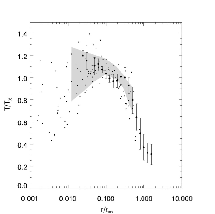
Figure 3: Mean spectroscopic-like temperature profile for all the clusters in Table 1. Each cluster profile is normalised by its mean spectroscopic-like temperature ($T_{X}$) within $r_{{}_{200}}$. The normalised profiles are averaged in order to obtain the plotted mean profile. Dots represent the different bins equispaced in logarithmic scale with width 0.1 dex, and error bars are 1 $\sigma$ s.d. The shaded region encloses the mean and 1 $\sigma$ s.d. temperature profiles from a representative sample of nearby clusters by  Pratt et al. (2007). The small black dots correspond to the temperature profiles of the clusters in the sample of  Vikhlinin et al. (2005).

Figure 4: Mean entropy profile for all clusters in Table 1 compared with the fitting in Voit, Kay & Bryan (2005). The radial profiles for each cluster are obtained using equispaced logarithmic bins. All of them are normalised to their respective values of $S_{{}_{200}}$, and then, the mean profile is obtained. Continuous line represents the mean profile and error bars show 1 $\sigma$ s.d. Dashed line shows the fitting by Voit, Kay & Bryan (2005).

In Figure 1 the different merger events can be easily identified. Whereas the relaxed cluster (right panel) has a quiet evolution, the middle panel shows a cluster suffering three mergers between $z=0.79$ and $z=0.65$. By comparing the masses of the different halos involved in these processes, all the events are classified as minor mergers. In the left panel, a cluster undergoing several mergers at different times is presented. Some of the mergers are minor ones, but there are major collisions at $z=0.99,z=0.79$ and $z=0.72$. In order to quantify the effect of mergers, we will correlate all these phases of activity in the clusters evolution with changes and effects on the different physical quantities.

It is important to notice that some of the merger trees also show halos that break apart, that is, lose mass and reduce their sizes. This process operates at two well separated regimes with different causes. The first group is formed by very small size halos. These halos are not really gravitationally bound and they can be easily disrupted by interactions with environment or with other halos. For the halos with larger masses, those mass losses are small, and they are associated with tidal interactions.

Figure 5: Gas entropy at $0.1\,r_{{}_{200}}$ as a function of temperature, $T_{200}$. Simulated clusters are represented by filled circles, whereas observational data with error bars stand for the  Ponman, Sanderson & Finoguenov (2003) sample. In order to compare simulations and observations, $T_{{}_{200}}\equiv T_{X}$ has been assumed.

3.2 Average radial profiles

In order to analyse the main properties of the simulated galaxy clusters, we compute radial profiles for several quantities. These profiles are centred at the centre of mass of each halo and run outwards from the centre to a distance slightly larger than the radius, $r_{200}$. The bins are equispaced in logarithmic scale with widths 0.1 dex. In all the plots displaying radial profiles, the radial coordinate is normalised to the $r_{200}$ at this time.

In Figure 2, we plot averaged radial profiles for several quantities for the clusters in the reduced sample (see Table 1). All the profiles are scaled by the plotted quantities at $r_{200}$ defined according to Eqs.(8)-(10). The mean profiles (continuous lines) are computed by averaging all the profiles of the clusters of each class. The right column stands for the relaxed clusters, the central column represents the minor merger clusters, and the left column displays the major merger clusters. The plotted quantities are gas ($\rho/\rho_{200}$) and dark matter ($\rho_{dm}/\rho_{200}$) densities, temperature ($T/T_{200}$), and entropy ($S/S_{200}$). The continuous lines stand for results at $z=0$ and shadowed regions mark one $\sigma$ deviation. Let us stress that, in Figure 2 and in the following ones – unless explicitly stated –, we consider mean profiles rather than median profiles.

A detailed analysis of Fig. 2 shows the main features of the three categories in which we have classified the different clusters. The comparison of gas and dark-matter density profiles does not show notable differences. Whereas for the gas density, the relaxed clusters exhibit a slightly higher density at the centre compared with the minor and major merger clusters, the behaviour for the dark matter is the opposite, having the major merger clusters a higher density. In any case, the profiles are consistent with the expected characteristics of density profiles for galaxy clusters.

Concerning the temperature profiles, there are no dramatic differences either. All clusters, in the reduced sample, show a central core with an almost constant temperature and a declining profile outwards. This result is compatible with observational data (e.g.,  De Grandi & Molendi (2002)), and with the idea of a quite universal temperature profile for the galaxy clusters  (Loken et al., 2002). The major and minor merger cluster profiles have very similar central temperatures, although the isothermal core is larger for the major merger clusters. The relaxed clusters have a bigger isothermal core with a slightly lower value of the temperature compared with the major and minor merger clusters.

Figure 6: Radial profiles of entropy ($S$) and temperature ($T$) at different redshifts. Left column shows the result for a cluster representing the major merger clusters, central column for a minor merger cluster and right column for a relaxed cluster.

The temperature profiles of the most massive clusters in our reduced sample do not exhibit a drop in the temperature in their central regions. Apparently, this could seem to differ from the results of the simulations by  Kay et al. (2007) or the observational data presented by  Vikhlinin et al. (2005) or  Pratt et al. (2007). These last observational results show clusters with temperature profiles with drops in their central temperatures. This effect is more outstanding in the case of  Vikhlinin et al. (2005). The nature of this discrepancy amid both observational results could be related with the use of different instrumentation in order to obtain the data of both samples. It must be noticed that whereas  Pratt et al. (2007) used XMM-Newton, the results of  Vikhlinin et al. (2005) were obtained using CHANDRA – with higher angular resolution. This could explain that some cool cores in the  Pratt et al. (2007) sample were not properly resolved. In order to compare with the results in  Pratt et al. (2007) and  Vikhlinin et al. (2005), we have calculated the spectroscopic-like radial temperature profile for each cluster of our reduced sample (clusters listed in Table 1) and normalised them to their respective mean $T_{sl}$ within $r_{{}_{200}}$, that we denote as $T_{X}$. In Figure 3, we compare the mean of all these radial temperature profiles, represented by dots with error bars (one $\sigma$ standard deviation), with the observational results in  Pratt et al. (2007) marked as the shaded region, and the results in  Vikhlinin et al. (2005) represented by small dots . Our results are consistent with these observational data in an average sense, being slightly more similar to the data of  Pratt et al. (2007).

We can understand our result, if we keep in mind that the clusters we are considering are the most massive ones in our sample. As we will discuss in more detail in Sec. 3.4, we have found that there is a strong anticorrelation between the drop of temperature in the central region and the mass of the cluster. Therefore, the larger the mass of the cluster the smaller the number of clusters with central gradients of temperature. However, if all the clusters in the complete sample are considered, then a relevant fraction of the population ($\sim 16\%$) shows temperature profiles with central gradients (see Sec. 3.4 for more details).

More interesting is the analysis of the entropy profiles. In all cases, the clusters have entropy cores and profiles outside $0.2\,r_{200}$ compatible with a power law $S(r)\propto r^{\alpha}$  (Tozzi & Norman, 2001). In previous work carried out by  Voit, Kay & Bryan (2005), the authors performed several non-radiative SPH and AMR simulations, and studied the main features of the entropy profiles of the galaxy clusters in their numerical samples. Besides several differences in the inner cores, all clusters in their sample, regardless of the numerical technique used, showed very similar entropy profiles outside a region around $0.2\,r_{200}$. In particular, for the AMR simulation, they found that the entropy profile in the outer regions can be better fitted by the power law $S(r)=1.43\,S_{200}(r/r_{200})^{1.2}$. In Figure 4, we compare the mean entropy profile of all the clusters in Table 1 with the fitting by  Voit, Kay & Bryan (2005). Continuous line represents our mean entropy profile with $1\sigma$ error bars. Dashed line stands for  Voit, Kay & Bryan (2005) fitting. Our results seem to be compatible with the fitting in the outer part of the profiles, whereas in the inner region, where cooling and feedback processes could be relevant, differences are expected.

In order to compare our results with observational data, we have looked at the values of the entropy at $0.1\,r_{{}_{200}}$, $S_{{}_{0.1\,r_{200}}}$, and compared them with previous data by  Ponman, Sanderson & Finoguenov (2003). In Figure 5 we plot the observational data (with error bars) by  Ponman, Sanderson & Finoguenov (2003) together with the values for the clusters in our reduced sample with temperatures higher that $1\,keV$ (filled circles). The points representing simulated clusters match well with the observational data apart from three clusters that are marginally compatible. These three objects turn out to have some peculiarities as they have suffered quite recent merger events. The values of the entropy at the very center of the simulated clusters are also similar to recent Chandra observations  (Morandi & Ettori, 2007). Therefore, our results seem to be reasonably compatible with the observations taking into account all the simplifications and limitations of our approach.

Coming back to the comparison of the results according to the merger history of the clusters, the generic shape of the entropy profiles does not depend systematically on the mass or temperature of the clusters, in agreement with observations  (Ponman, Sanderson & Finoguenov, 2003). The sizes of the cores are similar in the relaxed and minor merger clusters and slightly larger in the major merger ones. As it would be naively expected, the entropy floor in the relaxed clusters is lower than for the minor merger clusters, and this one is also lower than for the major merger clusters. Although the differences seem not to be dramatic, they are clearly visible in the mean profiles. These differences in the value of the entropy in the core, would be a clear consequence of the different evolutionary histories of each cluster.

Figure 7: Time evolution of the average entropy ($S_{0.1r_{200}}$) within the inner 10% of the radius $r_{{}_{200}}$, the ratio between total internal ($E_{{}_{U}}$) and kinetic ($E_{{}_{K}}$) energies, and the X-ray luminosity ($L_{{}_{X}}$), both evaluated within $r_{{}_{200}}$. Left column shows the result for a cluster representing the major merger clusters, central column for a minor merger cluster and right column for a relaxed cluster. Vertical lines delimit the time interval when mergers occur.

3.3 Merger effects

Merger events can produce shocks and compression waves in halos. Their effects could be an efficient way to transfer part of the gravitational energy associated to the collisions to the ICM of the final halo after the mergers. In this picture, the role of turbulence and mixing phenomena is crucial as a way to redistribute this energy into the ICM.

The study of these scenarios requires a numerical scheme able to tackle with an accurate description of shock waves, strong gradients as well as to describe the turbulence associated to those violent events. As it has been discussed in Sec. 1, the ability of different numerical techniques to describe these phenomena is still a matter of debate.

We focus in this Section on the effects of different merger events in the thermodynamical properties of the ICM. In order to do so, we select the same three clusters than in Sec. 3.1. Each one of them represents one of the three groups of clusters, and as it was already mentioned, they have been chosen in such a way that they have similar masses and sizes at $z=0$.

In order to discuss the effects of different merger events in the thermodynamical properties of the ICM, we show in Figure 6 the radial profiles of entropy ($S$) and temperature ($T$) at several redshifts for the selected clusters. This figure can be correlated with Fig. 1 to detect the effect produced by the merger events. Lines representing high redshifts must be taken carefully. They correspond to early stages of the clusters formation when these structures are far from being relaxed and, therefore, the radial profiles are not really meaningful.

The relaxed cluster shows a higher entropy and temperature at high redshifts, with a tendency to reach a relaxed state around $z\sim 0.5$ with small changes. The tendency for the minor merger cluster is similar for the lines displaying $z\sim 2$ and $z\sim 1$, that is, a reduction of the value of the entropy core. However, associated with the minor merger events, there is a significant increase in the value of the entropy core which, eventually, ends up in a reduction of the temperature and entropy at $z\sim 0$ with respect to the values at $z\sim 0.5$. In the case of the major merger cluster, between $z\sim 1$ and $z\sim 0.6$ when the major mergers take place, there is an increase in the entropy and a reheating as the temperature also increases. Later on, the cluster cools to a lower temperature but part of the energy of the merger has been released in the cluster which has a higher entropy. It must be noticed that the values for the entropy are considerably larger than for the other two clusters previously discussed.

So as to assess more clearly the effects of mergers in the thermodynamical properties of ICM, we show in Figure 7 the time evolution of several quantities: the averaged entropy within the 10% of $r_{{}_{200}}$ ($S_{0.1r_{200}}$), the ratio of the total internal to kinetic energies ($E_{{}_{U}}/E_{{}_{K}}$), and the integrated X-ray luminosity ($L_{X}$), both within the radius $r_{{}_{200}}$. As in previous plots, each column represents the results of a cluster representing one of the three classes.

For the relaxed cluster, the situation is simple. The early stages of cluster formation have left high entropy and internal energy. However, with the time evolution, the cluster cools and loses internal energy, creating a lower entropy core, and increasing the X-ray luminosity. The minor merger cluster exhibits a different history. As the cluster forms a bit later than the previous one, it begins with a lower entropy and internal energy compared with the relaxed cluster. The time zone when mergers happen – delimited by the vertical lines – can be clearly connected with important changes in the cluster evolution. The first minor merger boosts the entropy level and the internal energy, indicating that some energy has been injected in the system. This energy reheats the ICM and produces a decrease in the luminosity by delaying the cooling. Later on, the cooling takes over again dumping part of the energy, but leaving a net increase in the entropy. The history of the major merger cluster is slightly different. At the initial phase, the smooth accretion has produced an increasing trend in the core entropy, the internal energy and the luminosity. After the major merger the situation is different. Due to the more dramatic effects of the major mergers (higher disruption, stronger shock waves, and more turbulence and mixing) there is an increase in the entropy level, but associated with an immediate loss of energy due to radiation. Another minor merger produces some minor changes but the final state is a cluster pretty similar to the previous ones but with a significantly higher entropy.

3.4 Cool cores and cluster mergers

Figure 8: Fraction of all galaxy clusters in our simulation that have CC vs the gaseous mass of the clusters. The simulated clusters (continuous line) and the observed clusters from  Chen et al. (2007) (dashed line) and  O’Hara et al. (2006) (dotted line) are binned in five linearly equispaced bins.

It is well known that clusters of galaxies exhibit an important feature that allows to classify them into two separate populations, those having cool cores (CC) and those others not having cool cores (NCC).

Recently,  Chen et al. (2007) concluded that, roughly, half of the population observed in a sample with more than hundred clusters have CCs. The explanation for this dichotomy is not clear and it remains a matter of debate. Several authors have studied this problem by means of numerical simulations. Thus,  Kay et al. (2007) overestimate the number of CC clusters since almost all their clusters show the presence of CCs. However,  Burns et al. (2008) claimed to be the first authors producing a simulation with CC and NCC clusters in the same numerical volume, although their abundance at $z\sim 0$ of CC clusters, $\sim 16\%$, seems to be lower than the observed fraction by  Chen et al. (2007), $\sim 46\%$. Interestingly, the results presented by  Kay et al. (2007) are based on SPH simulations, whereas those of  Burns et al. (2008) are obtained using an Eulerian AMR code. It is likely that feedback processes could be directly involved in the survival of CCs in clusters, but it is also possible that mergers could play an important role erasing the presence of CCs  (Poole et al., 2006; Burns et al., 2008). In this Section, we analyse our simulation paying special attention to the presence of CCs, and their relative abundances.

Figure 9: Fraction of CCs as function of redshift for the simulated clusters in our complete sample. Error bars show $\sqrt{N}$ uncertainties due to the number counts.

Following  Burns et al. (2008), we define a CC cluster as one with a $\geq 20\%$ reduction of its central temperature compared with the surrounding region. Using this definition, we have classified all the clusters in our complete sample – an extended sample containing all the clusters in the simulation – into two groups: CCs and NCCs.

In Figure  8, we plot the fraction of CCs as a function of gaseous mass at $z=0$. We have binned the clusters using five linearly equispaced bins in the range $[10^{13},10^{15}]\,M_{\odot}$. The continuous line shows our results. For the sake of comparison, we have used the samples of  O’Hara et al. (2006) and  Chen et al. (2007), and we have binned the clusters in these samples using the same bins than for our results. The dashed and dotted lines correspond to Chen’s and O’hara’s results, respectively.

Our results are extremely similar to those of the  Burns et al. (2008) simulation, where they found a total fraction of $\sim 16\%$ CC clusters (see figure 8 in this reference) and in our case the number is also $\sim 16\%$. As in  Burns et al. (2008), our results differ in the absolute numbers from the observational data, but more interestingly, we have confirmed the general trend of a decreasing number of CC clusters with cluster mass.

Although, we have no clear explanation for the discrepancy between the absolute number of CC clusters in our simulation and the observational data by  Chen et al. (2007), two plausible explanations can be given in order to interpret these results. The first one has to do with the fact that no metal-dependent cooling has been considered in the simulation. It is known (see for instance  De Grandi & Molendi (2002); Vikhlinin et al. (2005)) that some clusters can show strong metallicity gradients, with metallicities rising to solar in the central regions. This limitation of the present simulation could produce some artificial reduction of the cooling, specially in systems where $kT<2\,keV$. Therefore, this shortcoming could mimic, effectively, some sort of uncontrolled non-gravitational feedback. The second possibility is related with a resolution issue, as no resimulations of the clusters have been performed. Therefore, despite the use of an AMR code, there could exist some resolution limitations. This last possibility seems much less important, though.

We have also looked at the time evolution of the fraction of CC clusters. In Figure  9, we plot the fraction of CCs in our sample as a function of the redshift from $z\sim 2$ until $z=0$. Again, our results are fully consistent with the simulations by  Burns et al. (2008) and show no important change in the fraction of CCs backwards in time, at least back to $z\sim 1$. Our results are in contradiction with observational evidences showing an important variation in the fraction of CCs from $z=0.5$  (Vikhlinin et al., 2006).

Before $z\sim 1$, we find a dramatic reduction in the fraction of CCs with time. As it would be expected, the abundance of CCs would be directly correlated with the hierarchical formation of the clusters. At the epoch of cluster formation, almost none of the clusters would have a CC. The formation of CCs would require the establishment of cooling flows which, eventually, and through a slow process will form the cool cores. However, once the clusters were fully formed, the major mergers would destroy the CCs, creating a population of NCC clusters. It is clear that feedback processes would also play a crucial role in this mechanism, but in the present simulation, where no relevant feedback mechanism – apart of the gravitational – has been taken into account, the effect of mergers on the existence of CCs is more outstanding. As the mergers are more dramatic in the more massive systems, this would explain the anticorrelation of the fraction of CCs and the mass of the clusters (see Fig. 8).

In order to deepen our knowledge of the connection between merger activity and the presence of CCs in clusters, we have studied the dependence of the fraction of relaxed clusters with the cluster mass. If mergers play an important role in the existence of CCs, one would expect that the systems that have evolved quietly (no recent mergers) do have cool cores. The comparison between the fractions of CC clusters and relaxed clusters is not direct as the establishment of cooling flows and the subsequent formation of CCs could require long time scales, specially for the smaller systems. In any case, and taking the result with caution due to all the uncertainties, we have computed the fraction of relaxed clusters which have central cores with cooling times shorter or comparable to the elapsed time from the clusters formation ($z_{for}$, see Sec. 3) until the actual time ($z=0$). Therefore, these clusters would have had time to set up a CC. The result shows the same trend than that in Fig. 8, that is, the number of relaxed cluster (no mergers) decreases with the cluster mass. This comparison would show that the smaller systems tend to have a CC and a quite evolution (no merger events), whereas the larger systems suffer the most important merger events and are NCC systems.

3.5 Scaling relations

Figure 10: Scaling relations for our galaxy cluster sample. The panels display, from top to bottom: integrated X-ray luminosity, mass, and mean entropy within the radius $r_{{}_{500}}$. In all the panels, the previous quantities are plotted against the temperature, $T_{{}_{500}}$, computed according to Eq. 9. The different symbols represent the clusters in the sample, the continuous lines stand for the proper fittings, and the small filled dots represent observational data by  Horner (2001) and  Ponman, Sanderson & Finoguenov (2003), respectively.

The scaling relations are crucial tools to study the galaxy clusters, as they connect observables like X-ray luminosities, with cluster properties, namely, masses and temperatures. Moreover, they can be an excellent way to check the behaviour and consistency of the simulations, by comparing with the scaling relations obtained in other simulations or with observations.

The galaxy cluster reduced sample studied in this paper is biased towards the most massive clusters of our simulation. Therefore, the statistical properties of this sample must be taken with caution as the sample is far from being complete, due to the numerical limitations. In the present subsection, we have extended the reduced sample (see Table 1) by considering all clusters, in the complete sample, with temperature, $T_{{}_{500}}\geq 1\,\,keV$ (see Eq. 9).

In Figure 10, several scaling relations are plotted: X-ray luminosity (upper panel), mass (middle panel), and mean entropy (bottom panel) within the radius $r_{{}_{500}}$. All these three quantities are plotted against the temperature $T_{{}_{500}}$. Our results can be fitted by the following scaling relations: $L\propto T^{2.5}$, $M\propto T^{1.5}$, and $S\propto T^{0.9}$. In the three relations, we have plotted all the clusters with temperatures $T_{{}_{500}}\in[1.0,8.0]\,keV$. This choice slightly increases the number of clusters of the original sample presented in Table 1. For completeness, and in order to compare with observational data, we have compared our scaling relations with data by  Horner (2001) for the $L-T$ relation and by  Ponman, Sanderson & Finoguenov (2003) for the $S-T$ relation, respectively. These data are displayed as small dots in the top and bottom panels in Fig. 10. The results for our simulated sample seem to be consistent with observational data, leaving aside all the uncertainties of such direct comparison.

Focusing on the effect of mergers, and for the sake of comparison with previous works, let us assume that clusters that have had a relatively quiet evolution would likely develop a CC, whereas those clusters involved in merger events would see their cool cores distorted, turning into NCC clusters (see Sec. 3.4). Under this assumption, we could consider that the galaxy clusters in our sample, labelled as major and minor mergers, could be identified, broadly speaking, with NCC clusters like the ones studied by  Poole et al. (2008), and analogously, our relaxed clusters would be the CC clusters in this reference. The results displayed in Fig. 10 show some degree of segregation, with most of the major and minor merger clusters located at well separated regions on the scaling relation plots. The minor merger clusters sit, preferentially, at an intermediate region between the major merger clusters and the relaxed clusters. As a gross trend, the majority of clusters which have suffered mergers, are placed in zones with higher temperature and higher luminosity, mass, and entropy, respectively.

Mergers, specially the major ones, typically boost clusters along the L-T relation but not parallel to this relation. In Figure 11, we plot – for the major merger clusters in Table 1 – the overall drifts experienced by these clusters from $z=1.5$ until $z=0$. This evolution is illustrated by vectors starting (finishing) at the values for L and T at $z=1.5$ ($z=0$). All the vectors could be decomposed in two components representing the change in temperature and luminosity. Two special clusters deserve a particular discussion. The first one, represented by a triangle, has no arrow associated. This is due to the fact that this cluster has been classified as major merger but it marginally satisfies the 1:3 condition in the mass ratio. Therefore, it is a transition case between major and minor clusters, according to our definition of merger. However, as we will discuss later, consistently with its evolution in the L-T plane, it behaves like the minor merger clusters. The second particular case, represented in the plot by a star, shows the evolution of a cluster with a extremely strong cooling flow at $z=1.5$. A careful study of the radial temperature of this cluster at that time, shows an extremely relevant CC. During the evolution, the merger event substantially reduces the cooling flow, and disturbs the CC, although the cluster remains radiating. Interestingly, all clusters, except the one represented by the triangle, show a net increase in temperature. Concerning luminosity, letting aside the two particular cases just mentioned, the rest of clusters shows an increase in luminosity. We have performed a similar analysis for the minor merger clusters, and they do not show any clear trend and seem to behave very similar to the relaxed clusters.

There is a clear bias in the treatment of small clusters and groups. Nevertheless the results of our simulation are consistent with previous results, specially considering that it has not been introduced any other pre-heating or feedback mechanism, besides the one from the star formation (very poor in the present simulation) and the so-called gravitational feedback (shock waves, mergers, etc). In any case, even though the sample can be limited, we wish to stress that the individual properties of each of the most massive clusters are well defined.

Figure 11: The X-ray luminosity vs the temperature, $T_{{}_{500}}$, within radius, $r_{{}_{500}}$. The plot shows, as vectors, the overall drifts experienced by the most massive major merger clusters in their positions at the L-T relation from $z=1.5$ until $z=0$. The clusters, at $z=0$, are labelled by squares, except two particular cases, identified by a triangle and a star, discussed in the text. Dashed line stands for the fitting of the L-T relation for the whole sample.

4 Discussion and conclusions

We have presented the results of a hydro and dark matter simulation of a moderate size volume of the Universe in the framework of a concordance cosmological model. The simulation follows the evolution of gaseous and dark matter components. Other relevant processes, like heating and cooling for a primordial gas, have been also taken into account.

The main idea of the present paper has been to study the role of galaxy cluster mergers as source of feedback of the ICM. The general picture of our simulation shows how mergers stirred the ICM by producing shocks and sound waves in scales comparable to the dimension of the cluster. These phenomena produce turbulence in the form of large eddies characterised by Reynolds numbers, $Re\sim 10^{3}$, which are values accessible to present-day numerical simulations  (Ricker & Sarazin, 2001).

Recent work by  Agertz et al. (2007) has shown, in some idealised situations, how the different numerical techniques, namely SPH and AMR, produce different results when describing the formation and evolution of eddies (Kelvin-Helmholtz) instabilities. According to this last reference, there are no substantial differences in results obtained with both techniques if the evolution time is smaller than the characteristic time of formation for Kelvin-Helmholtz instabilities, $\tau_{KH}$. This characteristic time can be estimated for the case of a cluster merger assuming similar densities for the clusters, a characteristic length scale of a few hundred of $kpc$, and a relative velocity of the order of one thousand km/s; with all this conditions, $\tau_{KH}$ turns to be of the order of a few hundreds of millions of years.

In the particular case of galaxy cluster mergers, the typical time scales of evolution after a merger are much larger than this $\tau_{KH}$, and therefore, it is likely that the particular numerical scheme used to simulate such scenario could play some role in the results. This has motivated us to study this problem by means of an AMR technique, and as a complementary work to the studies already published. Therefore, we have used an AMR Eulerian code specially designed for cosmological applications, with excellent capabilities to deal with strong gradients, shock waves, and low density regions. These kind of codes also describe properly some instabilities phenomena such as Kelvin-Helmholtz, Rayleigh-Taylor and, in general, turbulence and mixing processes (see the recent work by  Mitchell et al. (2009)).

In order to study the effect of mergers as feedback source, we have extracted and followed the evolution of the galaxy cluster like halos in our simulation. These halos have been studied directly from the simulation and without any resimulating scheme. This has implied a limitation due to numerical restrictions. Since the numerical scheme has the tendency to better resolve the most massive halos, our sample is biased towards these systems. However, it is in those large systems where the effects of mergers would be more relevant. On the other hand, this apparently drawback of lack of resolution on small halos, is compensated by the advantage that mergers can be followed in a consistent way as they naturally occur in the evolution of the simulated volume of the Universe. Thus, no controlled collisions have to be imposed a priori.

We have assumed a definition of galaxy cluster merger depending on the mass ratio of the halos involved in the merger. As additional condition, we have introduced a time limitation, in such a way that only mergers occurring in the recent past are taken into account. Thus, if masses are similar – between 1 and 1/3 – we define those events as major mergers. Events with larger ratios in masses are classified as minor mergers. Finally, clusters evolving without relevant merger events are designed as relaxed. Once we have assumed this criterion to group the clusters in our simulation, we have studied the radial profiles of each cluster for the gas and dark matter densities, temperature and entropy. In order to compare the main differences among the three classes, we have computed average profiles for each group. The forms of the different profiles are basically the same for the three categories, indicating no substantial changes in the physics of clusters. However, there is a trend in the normalisation. The relaxed and minor merger clusters have similar values of all quantities, whereas the major merger clusters are slightly hotter and with higher entropy.

The previously mentioned trends in entropy and temperature of clusters depending on their evolutionary history, can be quantify by looking at a representative cluster of each class and comparing the time evolution of their profiles of temperature and entropy.

In the same manner, the effects associated with cluster mergers can be traced in the time evolution of global quantities like the entropy in the inner 10% of the virial radius, the ratio of internal to kinetic energy, or the X-ray luminosity.

In all cases, cluster mergers release energy which ends up partially in the final object. The amount of energy locked in the final cluster is significantly larger for cluster mergers of similar masses (major mergers).

We have also considered all the clusters in the simulation without differentiating amid the merging activities. These results have been compared with previous simulations  (Voit, Kay & Bryan, 2005; Burns et al., 2008; Kay et al., 2007) and with observational data  (Ponman, Sanderson & Finoguenov, 2003; Vikhlinin et al., 2005; Pratt et al., 2007), paying special attention to the entropy and temperature profiles. Our results seem to be consistent with both, simulations and observations, in an average sense. However, there are still important differences like the lack of central drops in the temperature profiles of the most massive clusters.

The fraction of clusters in our sample that has cool cores has been computed at several redshifts. At $z=0$, our results are fully compatible with previous AMR simulations by  Burns et al. (2008), although seem to differ with the results of the SPH simulation by  Kay et al. (2007). We have compared the fraction of cool cores in our simulation with the observational data by  Chen et al. (2007) showing a similar trend, that is, the number of clusters with cool cores decreases with the cluster mass.

Given the fact that in our simulation the gravitational feedback is the relevant feedback mechanism, we have tried to correlate the merger events with the existence of cool cores. In order to do so, we have computed the fraction of relaxed clusters (no merger activity) as a function of the cluster mass. Interestingly, the fraction of clusters with cool cores, and the fraction of relaxed clusters as function of the cluster mass, show a very similar trend. Unfortunately, the absolute numbers of CCs in our simulation and the observations are quite different. We suggest two possibilities explaining this discrepancy. The first one would be related with the fact that no metal-dependent cooling has been considered in the simulation. This simplification could make the cooling more inefficient, specially at the central regions of the clusters. The second reason would be linked with a lack of resolution, which appears to be quite unlikely given the actual features of the considered simulation. In any case, it seems clear that there is an evident link between the merger events and the no existence of cool cores.

On the other hand, the time evolution of the fraction of cool cores shows that this quantity has not changed substantially from $z\sim 0$ to $z\sim 1$. This result is compatible with previous simulations  (Burns et al., 2008) but in disagreement with observational data  (Vikhlinin et al., 2006).

The cluster sample analysed in this paper is limited due to the fact that no resimulations have been done, and therefore, although an AMR code has been used, there are still resolution limitations. Nevertheless, we have analysed the scaling relations derived from our sample. Our results for $L\propto T^{2.5}$, $M\propto T^{1.5}$, and $S\propto T^{0.9}$ are consistent with previous results that do not introduce any extra reheating or feedback.

We have found some degree of segregation in the scaling relations depending on whether the clusters have or have not undergone a recent merger. The systems that have experienced merger events are usually located at high temperatures, luminosities, masses, and entropies, respectively, at the different scaling relation plots. These results could be comparable with recent works looking at the existence or not of cool cores in clusters  (Burns et al., 2008; Poole et al., 2008). The analysis of the time evolution of major merger clusters in the L-T relation, has shown that these clusters have a tendency to move towards regions of this relation with higher temperature and luminosity. This tendency is similar to that found by  Hartley et al. (2008), where authors investigate the L-T relation in a large simulation with a strong preheating.

A clear improvement for future work would be to increase the number of clusters in the sample by simulating larger volumes with higher resolution. Therefore, it would be feasible to reliably study the scaling relations for each one of the three families of clusters that we have considered in this paper. In any case, even when the sample can be limited, the individual properties of each of the most massive clusters are well defined.

The role of mergers as source of feedback, transferring part of the gravitational energy to the thermal energy, is still a matter of debate and study. Mergers are crucial to understand galaxy cluster formation and galaxy formation scenarios as they influence directly the ICM properties. Simulations with higher resolution and including more physical processes are needed in order to keep on quantifying the role of mergers in the hierarchical scenario of structure formation. In parallel, some results from simulations, like the ones presented here, can be considered in semi-analytical models in order to improve their description of the gas component.

APPENDIX A: Star formation

The star formation has been introduced in the MASCLET code following the ideas of Yepes et al. (1997) and Springel & Hernquist (2003). In our particular implementation, we assume that cold gas in a cell is transformed into star particles on a characteristic time scale $t_{*}$ according to the following expression:

$$\frac{d\rho_{*}}{dt}=-\frac{d\rho}{dt}=\frac{\rho}{t_{*}(\rho)}-\beta\frac{\rho}{t_{*}(\rho)}=(1-\beta)\frac{\rho}{t_{*}(\rho)}$$ (11)

where $\rho$ and $\rho_{*}$ are the gas and star densities, respectively. The parameter $\beta$ stands for the mass fraction of massive stars ($>8\,M_{\odot}$) that explode as supernovae, and therefore return to the gas component in the cells. We have adopted $\beta=0.1$, a value compatible with a Salpeter IMF. For the characteristic star formation time, we make the common assumption $t_{*}(\rho)=t^{*}_{o}(\rho/\rho_{{}_{th}})^{-1/2}$, equivalent to $\dot{\rho}_{*}=\rho^{1.5}/t^{*}_{o}$ (Kennicutt, 1998). In this way, we have introduced a dependence on the local dynamical time of the gas and two parameters , the density threshold for star formation ($\rho_{{}_{th}}$) and the corresponding characteristic time scale ($t^{*}_{0}$). In our simulations we have taken $t^{*}_{0}=2\,Gyr$ and $\rho_{{}_{th}}=2\times 10^{-25}\,g\,cm^{-3}$. From the energetic point of view, we consider that each supernova dumps in the original cell $10^{51}\,erg$ of thermal energy.

In the practical implementation, we have assumed that star formation occurs once every global time step, $\Delta t_{l=0}$ and, only in the cells at the highest level of refinement ($l=7$). Those cells at this level of refinement, where the gas temperature drops below $T<2\times 10^{4}\,K$, and the gas density is $\rho>\rho_{{}_{th}}=2\times 10^{-25}\,g\,cm^{-3}$, are suitable to form stars. In these cells, collisionless star particles with mass $m_{*}=\dot{\rho}_{*}\Delta t_{l=0}\Delta x_{l}^{3}$ are formed. In order to avoid sudden changes in the gas density, an extra condition restricts the mass of the star particles to be $m_{*}={\rm min}(m_{*},\frac{2}{3}m_{gas})$, where $m_{gas}$ is the total gas mass in the considered cell.

References

- Agertz et al. (2007) Agertz O. et al., 2007, MNRAS, 380, 963
- Arnaud & Evrard (1999) Arnaud M., Evrard A.E., 1999, MNRAS, 305, 631
- Balogh et al. (2001) Balogh M.L., Pearce F.R., Bower R.G., Kay S.T., 2001, MNRAS, 326, 1228
- Bialek, Evrard & Mohr (2001) Bialek J.J., Evrard A.E., Mohr J.J., 2001, ApJ, 555, 597
- Borgani et al. (2002) Borgani S., Governato F., Wadsley J., Menci N., Tozzi P., Quinn T., Stadel J., Lake G., 2002, MNRAS, 336, 409
- Borgani et al. (2004) Borgani S. et al., 2004, MNRAS, 348, 1078
- Borgani et al. (2008) Borgani S., Diaferio A., Dolag K., Schindler S., 2008, SSRv, 134, 379
- Bryan & Norman (1998) Bryan G.L., Norman M.L., 1998, ApJ, 495, 80
- Burns et al. (2008) Burns J.O., Hallman E.J., Gantner B., Motl P.M., Norman M.L., 2008, ApJ, 675, 1125
- Chen et al. (2007) Chen Y., Reiprich T.H., Böhringer H., Ikebe Y., Zhang Y.-Y., 2007, A&A, 466, 805
- Davé, Katz & Weinberg (2002) Davé R., Katz N., Weinberg D.H., 2002, ApJ, 579, 23
- De Grandi & Molendi (2002) De Grandi S., Molendi S. , 2002, ApJ, 567, 163
- Eisenstein & Hu (1998) Eisenstein D.J., Hu W., 1998, ApJ, 511, 5
- Ettori et al. (2004) Ettori S. et al., 2004, MNRAS, 354, 111
- Fabian et al. (1994) Fabian A.C., Crawford C.S., Edge A.C., Mushotzky R.F., 1994, MNRAS, 267, 779
- Frenk et al. (1999) Frenk C.S. et al., 1999, ApJ, 525, 554
- Gill, Knebe & Gibson (2004) Gill S.P.D., Knebe A., Gibson B.K., 2004, MNRAS, 351, 399
- Haardt & Madau (1996) Haardt F., Madau P., 1996, ApJ, 461, 20
- Hartley et al. (2008) Hartley W.G., Gazzola L., Pearce F.R., Kay S.T., Thomas P.A., 2008, MNRAS, 386, 2015
- Horner (2001) Horner D.J., 2001, Ph.D. Thesis, Univ. Maryland
- Kaiser (1986) Kaiser N., 1986, MNRAS, 222, 323
- Katz, Weinberg & Hernquist (1996) Katz N., Weinberg D.H., Hernquist L., 1996, ApJS, 105, 19
- Kay, Thomas & Theuns (2003) Kay S.T., Thomas P.A., Theuns T., 2003, MNRAS, 343, 608
- Kay et al. (2004) Kay S.T., Thomas P.A., Jenkins A., Pearce F.R., 2004, MNRAS, 355, 1091
- Kay et al. (2007) Kay S.T. et al., 2007, MNRAS, 377, 317
- Kennicutt (1998) Kennicutt, R.C., 1998, ApJ, 498, 541
- (27) Klypin A., Gottlöber S., Kravtsov A., 1999, ApJ, 516, 530
- Kravtsov, Nagai & Vikhlinin (2005) Kravtsov A.V., Nagai D., Vikhlinin A.A., 2005, ApJ, 625, 588
- Lacey & Cole (1993) Lacey C., Cole S., 1993, MNRAS, 262, 627
- Lin, Mohr & Stanford (2003) Lin Y.-T., Mohr J.J., Stanford S.A., 2003, ApJ, 591, 749
- Loken et al. (2002) Loken C., Norman M. L., Nelson E., et al , 2002, ApJ, 579, 571
- Markevitch (1998) Markevitch M., 1998, ApJ, 504, 27
- Mazzotta et al. (2004) Mazzotta P., Rasia E., Moscardini L., Tormen G., 2004, MNRAS, 354, 10
- McCarthy et al. (2007) McCarthy I.G., 2007, MNRAS, 376, 497
- Mitchell et al. (2009) Mitchell N.L., McCarthy I.G., Bower R.G., Theuns T., Crain R.A., 2009, MNRAS, in press, arXiv:0812.1750
- Molt et al. (2004) Molt P.M., Burns J.O., Loken C., Norman M.L., Bryan G., 2004, ApJ, 606, 635
- Morandi & Ettori (2007) Morandi A., Ettori S. , 2007, MNRAS, 380, 1521
- Muanwong et al. (2001) Muanwong O., Thomas P.A., Kay S.T., Pearce F.R., Couchman H.M.P., 2001, ApJ, 552, L27
- Navarro, Frenk & White (1995) Navarro J.F., Frenk C.S., White S.D.M., 1995, MNRAS, 275, 720
- Navarro, Frenk & White (1997) Navarro J., Frenk C. S., White S. D. M. , 1997, ApJ, 490, 493
- O’Hara et al. (2006) O’Hara T.B., Mohr J.J., Bialek J.J., Evrard A.E., 2006, ApJ, 639, 64
- Osmond & Ponman (2004) Osmond J.P.F., Ponman T.J., 2004, MNRAS, 305, 1511
- Pearce et al. (2000) Pearce F.R., Thomas P.A., Couchman H.M.P., Edge A.C., 2000, MNRAS, 317, 1029
- Ponman, Sanderson & Finoguenov (2003) Ponman T.J., Sanderson A.J.R., Finoguenov A., 2003, MNRAS, 343, 331
- Poole et al. (2006) Poole G. B., Fardal M. A., Babul A., McCarthy I.G., Quinn T., Wadsley J., 2006, MNRAS, 373, 881
- Poole et al. (2007) Poole G. B., Babul A., McCarthy I. G., Fardal M. A., Bildfell C. J., Quinn T., Mahdavi A., 2007, MNRAS, 380, 437
- Poole et al. (2008) Poole G. B., Babul A., McCarthy I. G., Sanderson A. J. R., Fardal A., 2008, arXiv:0804.1552
- Pratt et al. (2007) Pratt G.W., Böhringer H., Croston J.H., Arnaud M., Borgani S., Finoguenov A., Temple R.F., 2007, A&A, 461, 71
- Quilis (2004) Quilis V., 2004, MNRAS, 352, 1426
- Quilis, Ibáñez & Sáez (1998) Quilis V., Ibáñez J.M., Sáez D., 1998, ApJ, 502, 518
- Ricker & Sarazin (2001) Ricker P. M., Sarazin C. L., 2001, ApJ, 561,621
- Sanderson et al. (2003) Sanderson A.J.R., Ponman T.J., Finoguenov A., Lloyd-Davies E.J., Markevitch M., 2003, MNRAS, 340, 989
- Springel & Hernquist (2003) Springel V., Hernquist L., 2003, MNRAS, 339, 289
- Sutherland & Dopita (1993) Sutherland R., Dopita M.S., 1993, ApJS, 88, 253
- Theuns et al. (1998) Theuns T., Leonard A., Efstathiou G., Pearce F.R., Thomas P.A., 1998, MNRAS, 301, 478
- Tornatore et al. (2003) Tornatore L., Borgani S., Springel V., Matteucci F., Menci N., Murante G., 2003, MNRAS, 342, 1025
- Tozzi & Norman (2001) Tozzi P., Norman C., 2001, ApJ, 546, 63
- Valdarnini (2003) Valdarnini R., 2003, MNRAS, 339, 111
- Vikhlinin et al. (2005) Vikhlinin A., Markevitch M., Murray S.S., Jones C., Forman W., Van Speybroeck L., 2005, ApJ, 628, 655
- Vikhlinin et al. (2006) Vikhlinin A., Burenin R., Forman W.R., Jones C., Hornstrup A., Murray S.S., Quintana H., 2006, astro-ph/0611438
- Voit (2005) Voit G.M., 2005, Rev. Mod. Phys., 77, 207
- Voit, Kay & Bryan (2005) Voit G.M., Kay S.T., Bryan G.L., 2005, MNRAS, 364, 909
- White (2002) White M., 2002, ApJ, 143, 241
- Yepes et al. (1997) Yepes G., Kates R., Khokhlov A., Klypin A., 1997, MNRAS, 284, 235