Effects of Quantum Vacuum Fluctuations

of the Electric Field on DNA Condensation

Alfredo Iorio^(a),∗, Samik Sen^(b),∗∗, Siddhartha Sen^(c,d),†

^(a) Faculty of Mathematics and Physics, Charles University of Prague

V Holešovickach 2, 180 00 Prague 8 - Czech Republic

^(b) Rocwood 27, Stillorgan (Co. Dublin) - Ireland

^(c) School of Mathematical Sciences, University College Dublin

Belfield, Dublin 4 - Ireland

^(d) Indian Association for the Cultivation of Science

Jadavpur, Calcutta 700032 - India

By assuming that not only counter-ions but DNA molecules as well are thermally distributed according to a Boltzmann law, we propose a modified Poisson-Boltzmann equation at the classical level as starting point to compute the effects of quantum fluctuations of the electric field on the interaction among DNA-cation complexes. The latter are modeled here as infinite one-dimensional wires ($\delta$-functions). Our goal is to single out such quantum-vacuum-driven interaction from the counterion-induced and water-related interactions. We obtain a universal, frustration-free Casimir-like (codimension 2) interaction that extensive numerical analysis show to be a good candidate to explain the formation and stability of DNA aggregates. Such Casimir energy is computed for a variety of configurations of up to 19 DNA strands in a hexagonal array. It is found to be strongly many-body.

^∗ E-mail: alfredo.iorio@mff.cuni.cz

^∗∗ E-mail: samiksen@gmail.com

^† E-mail: sen@maths.ucd.ie

PACS: 87.15.ag; 87.15.-v; 87.15.bk

Keywords: Quantum calculations; Biomolecules: structure and physical properties; Structure of aggregates

1 Introduction

Dilute solutions of DNA upon the addition of specific multivalent cations have remarkable properties [1]. Initially the DNA molecules in aqueous solution ionize with two negatively charged phosphates strands remaining, giving rise to a highly charged anion with lineal charge density of one negative charge per $1.7$ Å. The system, in the presence of cations, binds them by a process known as the Oosawa-Manning (OM) condensation [2, 3] (for a review see, e.g., [1, 4, 5]). When about 90 per cent of the DNA negative charge is screened and when the cations have a specific valency $+k$, usually $k=3$ or $k=4$, the DNA strands collapse to form rod-like, spheroidal and toroidal aggregates, whose size can be experimentally controlled within limits [6].

There have been different approaches to study these features of DNA collapse and structure formation and much progress has been made over the last decade. Nonetheless, many aspects remain unclear. Broadly speaking, we can identify two avenues that have been explored:

In one the details of the helicoidal charge distribution of the DNA are used to compute the electrostatic interaction between two DNA strands using a linearized Poisson-Boltzmann (PB) (or Debye-Hückel (DH)) approach [7] (see also the review article [8]). Within this approach the attraction between two like-sign charged but suitably oriented DNA molecules and the specificity of cations driving the attraction can be predicted. However, it was also realized that when the molecules are three or more frustration comes about (for an assembly of several DNA molecules in an hexagonal array on a triangular lattice treated within this model see, e.g., [10] and also [11]). Thus, clearly, this force alone cannot account for the formation and stability of DNA aggregates.

In alternative approaches the surface of a single DNA molecule is treated as a two-dimensional complex system and statistical mechanical arguments lead to the counterion-mediated attraction between two DNA molecules [12, 13, 14, 15]. The key idea there is that the attraction is triggered by local correlations and thermal fluctuations not accounted for in the mean-field PB approach. These fluctuations being those of the number or charge density of the ions, they are constrained to be classical in nature.

In a recent paper [16] we explored the possibility for quantum vacuum fluctuations to be a viable candidate to drive the formation of DNA aggregates and to hold (“glue”) them together. In this paper we want to make explicit that analysis and shall present more details and numerical results to strengthen that hypothesis.

Our starting point is the modification of the PB classical equation to include the DNA macromolecules in the Boltzmann thermal distribution. This way delta-function potentials appear naturally in the equation to take into account the charge distribution of the DNA. Since classical electrostatic calculations are available and detailed [7] and since we do not expect our one-dimensional (delta-function) model to improve those calculations, we focus on the quantum corrections considered here via an effective action approach. When the electrostatic potential is small, as the OM condensation has taken place, we approximate our modified PB equation to obtain a modified DH equation where, as said, the DNA molecule-counterions complexes (which, for brevity, we shall often simply call “DNA strands”) are modeled as delta function potentials (carrying information relative to the charge distribution of the strand) as to be expected by general features of self-adjoint extension of differential (Hamiltonian) operators [18]. The resulting classical action is then taken as the start of a Renormalization Group (RG) type of analysis in which time-dependent quantum fluctuations of the electric field, propagating with the speed of light in the medium (and representing short distance effects) are averaged to generate an effective potential.

The nice outcome of this procedure is that it produces precisely the Casimir energy (for a review see, e.g., [19], [20] and [21]) in codimension 2 (lines in three dimensions) that was obtained in [22], as we demonstrate. There are two scales in the model: the original DH mass (inverse length) scale $\mu$, fixed by the parameters of the system, and a new mass (inverse length) scale $M$, introduced through a process of coupling constant renormalization, which is indeed a free parameter. These scales control the range of the interaction.

This energy is calculated for an assembly of $N$ strands ($N=2,4,7,19$) in arrays in a triangular lattice and we found that: i) it is attractive, irrespective of the charge of the DNA strands; ii) it has a range of ${\cal O}(10)$ Å in the simplest model considered; iii) the energy scale in the range is greater than $k_{B}T$; iv) there are important many-body effects. We then conclude that it is plausible that this quantum relativistic force is the “glue” holding together the aggregate of DNA strands.

The model presented here has limits. For instance, it suggests that the DNA strands collapse to a configuration of zero separation, due to an infinitely strong (singular) attractive energy at very short distances, an instance not occurring in real aggregates. This is an indication that this force is only one part of the puzzle and the full picture needs to include more. It seems to us that the key ingredients to have the full picture are three mechanisms: (i) the zero-point quantum interaction, that gives the universal attraction (“glue”); (ii) the “frustrated force”, that takes into account the detailed structure (finite size and helical architecture) and the active role of counterions (these alone seem to reproduce the helical architecture [17]); (iii) water-related forces, that need to be included.

In Section 2 we recall the basics of the derivation of the PB equation and then propose our modification of it to move on in Section 3 to the quantum calculation based on the averaging-over-fluctuations method. The latter is done in some details as this should make manifest what sort of interaction we are considering here and how we derive it. In Section 4 we present our numerical analysis of the interaction between several strands, starting with two, and discuss the outcomes and limitations of the model. The last Section is dedicated to our conclusions.

2 The modified Poisson-Boltzmann equation

Consider the electrostatic potential $\Phi(\vec{x})$ due to a charge density at finite temperature $\rho(\vec{x},T)$ placed in a medium with dielectric constant $\epsilon$. This obeys the Poisson equation

$$\nabla^{2}\Phi(\vec{x})=-\frac{4\pi}{\epsilon}\rho(\vec{x},T)\;.$$ (2.1)

Consider now the DNA molecule as a negatively charged rod immersed in water at room temperature ($T\simeq 300$K) with dissolved salt whose ions have valency $z=\pm k$, with $k=1,2,...$ (for instance, when the dissolved salt is NaCl, $k=1$, corresponding to Na⁺ and Cl^-). The charge distribution of the composite system DNA-salt is

$$\rho(\vec{x},T)=\rho_{\rm DNA}(\vec{x},T)+ke(n_{+}(\vec{x},T)-n_{-}(\vec{x},T))\;,$$ (2.2)

where $\rho_{\rm DNA}(\vec{x})$ is the charge density of the macroion, and we take

$$n_{\pm}(\vec{x},T)=n_{0}\exp\left(\mp\frac{ke\Phi(\vec{x})}{k_{B}T}\right)\;,$$ (2.3)

i.e. the concentration (density) of ions follows a Boltzmann distribution. Inserting (2.2) and (2.3) into (2.1) gives the PB equation

$$\nabla^{2}\Phi(\vec{x})=\frac{8\pi}{\epsilon}ken_{0}\sinh\left(\frac{ke\Phi(\vec{x})}{k_{B}T}\right)\;,$$ (2.4)

where only the region outside the surface of the macroion is considered, hence $\rho_{\rm DNA}=0$ (soon we shall re-introduce $\rho_{\rm DNA}$). Equation (2.4) is the widely used outcome of the mean-field theory that has been extensively applied to the study DNA molecules immersed into aqueous media with different salts and salt concentrations. Note that both coions (negative) and counterions (positive) are present due to the dissolved salt and that in experiments the counterions usually do not come only from the dissolved salt but are added separately.

Among the successes of the PB equation is the prediction of a phase transition – governed by the Manning parameter $\xi=l_{B}/b$, with $l_{B}=q^{2}/\epsilon k_{B}T$ the Bjerrum length (at room temperature $l_{B}\simeq 7.1$Å) and $1/b$ the lineal charge density that for DNA is $b=1.7$Å – where the counterions condense onto the DNA strands screening its negative charge to a large extent: when $\xi>1$ counterions stick to the charged rod to form a DNA-counterions complex. This is the OM condensation [2, 3].

Our concern is to study the interaction among DNA strands after at least 90 per cent of the negative charge has been screened via the OM condensation, as this is the reported critical value for collapse. It is then reasonable to consider $\Phi$ small. Furthermore, we explicitly consider the charge distribution $\rho_{\rm DNA}$ and demand that it obeys a Boltzmann distribution law as for the ions (see Eq.(2.3))

$$\rho_{\rm DNA}(\vec{x},T)=-n^{0}_{\rm DNA}(\vec{x})|q|\exp\left(\frac{|q|\Phi(\vec{x})}{k_{B}T}\right)\;,$$ (2.5)

where $q<0$ is the charge of the DNA strand with

$$n^{0}_{\rm DNA}(\vec{x})=\sum_{i=1}^{N}\nu_{i}(z_{i})\delta^{2}(\vec{x}_{\bot}-\vec{l}_{i})\;.$$ (2.6)

This charge density function defines our approximations: we model the DNA strands as infinite lines all parallel to the $z$-axis and located at $\vec{l}_{i}$ in the $x-y$ plane with the coefficients $\nu_{i}(z_{i})$ carrying information on the charge structure of the DNA strand. We further simplify our model by taking $\nu_{i}(z_{i})=\nu=$ constant, $\forall i=1,...,N$.

We now put everything together, expand the exponential and stop at first order to obtain

$$\left[-\partial^{2}_{z}-\nabla_{\bot}^{2}+\mu^{2}+\lambda\sum_{i=1}^{N}\delta^{(2)}(\vec{x}_{\bot}-\vec{l}_{i})\right]\Phi(\vec{x})=J\;,$$ (2.7)

which is a modified DH equation. Here $\mu^{2}=k^{2}\kappa^{2}$, with

$$\kappa^{-1}=\sqrt{\frac{\epsilon k_{B}T}{8\pi e^{2}n_{0}}}$$ (2.8)

the Debye screening length,

$$\lambda=\frac{4\pi\nu|q|^{2}}{\epsilon k_{B}T}$$ (2.9)

and

$$J=-\frac{4\pi\nu|q|}{\epsilon}\sum_{i=1}^{N}\delta^{(2)}(\vec{x}_{\bot}-\vec{l}_{i})\;.$$ (2.10)

In the following the operator in square brackets will often be indicated for brevity as $[-\nabla^{2}+V(\vec{x}_{\bot})]$, with obvious notations.

Delta function potentials are not new in physics (see, e.g., [23]). Their appearance in the present case can also be seen as the effect of removing points (the locations of the DNA strands) from the domain of the differential operator $-\nabla^{2}$. This naturally leads to delta functions as a compensation for the self-adjoint extension of such operator [18].

Eq.(2.7) can be used to compute classical electrostatic interactions. Nonetheless, we shall not do so as such calculations are available and detailed [7] and we do not expect our one-dimensional model to improve them. Thus, in the following Section, we shall focus on the quantum corrections.

3 Quantum fluctuations of the electric field

Let us consider small time-dependent fluctuations: $\Phi(\vec{x})\to\Phi(\vec{x})+\phi(\vec{x},t)$. $\Phi$ satisfies the modified DH equation (2.7) that descends from the action

$${\cal A}(\Phi)=\int d^{4}x\left(\frac{1}{2}\Phi[-\nabla^{2}+V(\vec{x}_{\bot})]\Phi+J\Phi\right)\;,$$ (3.11)

where we use units $\hbar=c=1$, with $c$ the velocity of light in the medium and, for the sake of clarity, we included an integration over time $\int_{0}^{\tau}dt$ even though the functions are time-independent. We then demand that to the fluctuation field $\phi$ as well is associated an action that is a suitable modification of (3.11), namely

$$\bar{{\cal A}}(\phi)=\int d^{4}x\frac{1}{2}\phi(-\partial_{t}^{2}-\nabla^{2}+V(\vec{x}_{\bot}))\phi\;.$$ (3.12)

Note that in $\bar{{\cal A}}(\phi)$ the term with the coupling to the “external current” $J$ is zero because

$$\int d^{4}xJ\phi=\int d^{3}xJ\int_{0}^{\tau}dt\phi=0\;,$$ (3.13)

as we impose $\int_{0}^{\tau}dt\phi=0$ as required for fluctuating fields. The field $\phi$, though, is a quantum field, hence the field configurations that satisfy the classical equations (the ones descending from $\delta\bar{{\cal A}}(\phi)=0$) are just on the same footing as all other field configurations[24]. The way to consider the effects of $\phi$ is to average these fluctuations out to obtain an effective action ${\cal A}_{\rm eff}(\Phi)$. This is done by considering the generating functional

$$Z[\Phi,\phi] = \int[D\Phi]e^{i{\cal A}(\Phi)}\int[D\phi]e^{i\bar{{\cal A}}(\phi)}$$ (3.14)

$$= \int[D\Phi]e^{-({\cal A}(\Phi)+{\rm corrections})}\;,$$ (3.15)

where we Wick rotate on the time direction $t\to it$, and identify ${\cal A}_{\rm eff}(\Phi)={\cal A}(\Phi)+$ corrections.

Thus we need to compute $I=\int[D\phi]e^{-\bar{{\cal A}}(\phi)}$ that, using standard Gaussian functional integrals methods (see, e.g., [25]), gives $I=[\det(-\partial_{t}^{2}-\nabla^{2}+V(\vec{x}_{\bot}))]^{-1/2}$ or

$$I=\exp\left(-\frac{1}{2}{\rm Tr}\ln(-\partial_{t}^{2}-\partial^{2}_{z}-\nabla_{\bot}^{2}+V(\vec{x}_{\bot}))\right)\;,$$ (3.16)

where the identity $\exp((-1/2)\ln\det A)=\exp((-1/2){\rm Tr}\ln A)$ was used and, as customary, the determinant and trace have to be computed in terms of the eigenvalues of the operator. To find such eigenvalues we suppose that

$$\phi(\vec{x}_{\bot},z,t)=\frac{1}{2\pi}\int_{-\infty}^{+\infty}dpe^{ipz}\phi_{p}(\vec{x}_{\bot})e^{i\omega t}\;,$$ (3.17)

and that $(-\nabla_{\bot}^{2}+V(\vec{x}_{\bot}))\phi_{p}(\vec{x}_{\bot})=E\phi_{p}(\vec{x}_{\bot})$. With this we obtain

$$I=\exp\left(-\frac{1}{2}\int_{-\infty}^{+\infty}\frac{d\omega}{2\pi}\int_{-\infty}^{+\infty}\frac{dp}{2\pi}\int_{0}^{+\infty}dE\rho(E)\ln(\omega^{2}+p^{2}+E)\right)\;.$$ (3.18)

Let us focus on $I_{p}(E)=(1/2\pi)\int_{-\infty}^{+\infty}d\omega\ln(\omega^{2}+E_{p}^{2})$, where $E_{p}^{2}=p^{2}+E$. One has that $\partial I_{p}(E)/\partial E=1/(2E_{p})$ which gives

$$I_{p}(E)=\int^{E}dE^{\prime}\frac{\partial I_{p}(E^{\prime})}{\partial E^{\prime}}=\frac{1}{2}\int^{E}dE^{\prime}\frac{1}{\sqrt{E^{\prime}+p^{2}}}=\sqrt{E+p^{2}}\;,$$ (3.19)

hence

$$I=\exp\left(-\frac{1}{2}\int_{-\infty}^{+\infty}\frac{dp}{2\pi}\int_{0}^{+\infty}dE\rho(E)\sqrt{E+p^{2}}\right)\;.$$ (3.20)

Thus the corrections to the classical action ${\cal A}(\Phi)$ are ${\cal E}\tau$ with the energy $\cal E$ given by

$${\cal E}=\frac{1}{2}\int_{-\infty}^{+\infty}\frac{dp}{2\pi}\int_{0}^{+\infty}dE\rho(E)\sqrt{E+p^{2}}\;.$$ (3.21)

This energy is of the form ${\cal E}=(1/2)\sum\omega$, i.e. the zero point Casimir energy of the system with $\sum$ replaced by $(1/2\pi)\int dp\int dE\rho(E)$ and $\omega$ by $\sqrt{E+p^{2}}$. Noticing that the density of states $\rho(E)$ contains information on the location $\vec{l}_{i}$ of the $N$ strands present in the system (see later discussion), clearly $\partial{\cal E}/\partial\vec{l}$ is a (Casimir) force.

The mathematical problem of determining the $\cal E$ of Eq.(3.21) has been solved in the context of scalar quantum fluctuations for interacting strings [22]. Let us give here a brief account of that derivation (see also [26]).

We first need to find the density of states $\rho(E)$. Define $H_{0}\equiv-\nabla^{2}+\mu^{2}$ and $H=H_{0}+\lambda\sum\delta^{(2)}(x-l_{i})\equiv H_{0}+W$. The Green’s functions are such that

$$(H-E)G(x,y)=\delta^{(2)}(x-y)\;,$$ (3.22)

where $<x|G|y>=G(x,y)$ and similarly for $G_{0}(x,y)$ with $H_{0}$. Hence, formally we have $G=1/(H-E)$ and $G_{0}=1/(H_{0}-E)$ which allows to set-up the Lipmann-Schwinger equation

$$G = \frac{1}{H-E}=\frac{1}{H_{0}-E}-\frac{1}{H_{0}-E}W\frac{1}{H-E}$$ (3.23)

$$= G_{0}-G_{0}WG=G_{0}-G_{0}WG_{0}+G_{0}WG_{0}WG=\cdots$$ (3.24)

$$= G_{0}-G_{0}W\frac{1}{1+G_{0}W}G_{0}\;,$$ (3.25)

or

$$G(x,y)=G_{0}(x,y)+\sum_{i,j=1}^{N}\frac{G_{0}(x,l_{i})G_{0}(l_{j},y)}{\sigma\delta_{ij}-G_{0}(l_{i},l_{j})}\;,$$ (3.26)

where $\sigma=-\lambda^{-1}$. Now define the energy eigenfunctions as $\psi_{n}(x)=<x|E_{n}>$ that give

$$\rho(E)=\sum_{n=0}^{\infty}\int d^{2}x|\psi_{n}(x)|^{2}\delta^{(2)}(E-E_{n})\;,$$ (3.27)

and use

$$G(x,y) = <x|\frac{1}{H-E+i\epsilon}|y>=\sum_{n=0}^{\infty}\psi_{n}(x)\frac{1}{E_{n}-E+i\epsilon}\psi^{*}_{n}(y)$$ (3.28)

$$= \sum_{n=0}^{\infty}\psi_{n}(x)\left({\cal P}\frac{1}{E_{n}-E}+i\pi\delta(E-E_{n})\right)\psi^{*}_{n}(y)\;.$$

Clearly

$$\rho(E)=\frac{1}{\pi}{\rm Im}\int d^{2}xG(x,x)\;.$$ (3.29)

We need now to prove an identity

$$\int d^{2}xG_{0}(x,l_{i})G_{0}(l_{j},x) = \int d^{2}x<x|\frac{1}{H_{0}-E}|l_{i}><l_{j}|\frac{1}{H_{0}-E}|x>$$

$$=<l_{j}|\frac{1}{(H_{0}-E)^{2}}|l_{i}> = \frac{\partial}{\partial E}<l_{j}|\frac{1}{H_{0}-E}|l_{i}>=\frac{\partial}{\partial E}G_{0}(l_{i},l_{j})\;.$$ (3.30)

With this and by using the expression (3.26) for the propagator in the expression (3.29) for the density of states we obtain

$$\rho(E) = \rho_{0}(E)+\frac{1}{\pi}\sum_{i,j=1}^{N}\frac{\partial G_{0}(l_{i},l_{j})/\partial E}{\sigma\delta_{ij}-G_{0}(l_{i},l_{j})}$$ (3.31)

$$= \rho_{0}(E)-\frac{1}{\pi}\frac{\partial}{\partial E}\sum_{i,j=1}^{N}\ln{\bar{\Gamma}}_{ij}\;.$$

where $\rho_{0}(E)=(1/\pi){\rm Im}\int d^{2}xG_{0}(x,x)$ and $\bar{\Gamma}_{ij}=\sigma\delta_{ij}-G_{0}(l_{i},l_{j})$. By dropping the $l$-independent $\rho_{0}(E)$ and by using the fact that ${\bar{\Gamma}}_{ij}$ is diagonalizable we obtain

$$\rho(E)=-\frac{1}{\pi}\frac{\partial}{\partial E}{\rm Tr}\ln{\bar{\Gamma}}_{ij}=-\frac{1}{\pi}\frac{\partial}{\partial E}\ln\det{\bar{\Gamma}}_{ij}\;.$$ (3.32)

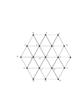
Figure 1: The configuration used for 19 DNA strands where $x$ is the distance between nearest neighbors.

The solution for $G_{0}(l_{i},l_{j})$, when the energy is Wick rotated to the real negative values is [22]

$$G_{0}(l_{i},l_{j})=\frac{1}{2\pi}K_{0}(\sqrt{E+\mu^{2}}l_{ij})\;,$$ (3.33)

where $K_{0}(x)$ is the modified Bessel function of the second kind of order zero and $l_{ij}=|l_{i}-l_{j}|$. Hence $G_{0}(L)\to\infty$ when $L\to 0$. One cures this divergence by splitting $G_{0}(L)$ into a finite part and a divergent part and renormalizing the coupling constant $\lambda$. This process introduces, for dimensional reasons, the scale $M$ that, for stability needs to be constrained: $M<\mu$ [22]. The result of this procedure is

$$\sigma-G_{0}(L) = -\frac{1}{\lambda}+\frac{1}{2\pi}\ln(ML)+\frac{1}{2\pi}\ln\left(\frac{\sqrt{E+\mu^{2}}}{M}\right)$$ (3.34)

$$\equiv -\frac{1}{\lambda(L)}+\frac{1}{2\pi}\ln\left(\frac{\sqrt{E+\mu^{2}}}{M}\right)$$ (3.35)

$$= \frac{1}{2\pi}\ln\left(\frac{\sqrt{E+\mu^{2}}}{Me^{2\pi/\lambda(L)}}\right)\;,$$ (3.36)

where we used the fact that $K_{0}(x)\sim-\ln x$ for small $x$. We now require $\lambda\to-\infty$ when $L\to 0$ so to have a finite $\lambda_{R}=\lambda(L)|_{L\to 0}$ and redefine the scale $M\to Me^{2\pi/\lambda_{R}}\equiv M$ which we still require to satisfy $M<\mu$.

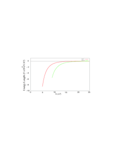
Figure 2: Energy of interaction of two DNA strands. The lower (upper) curve corresponds to $a=2$ ($a=1$). Distances $x$ are measured in units of $1/\mu\sim$ ${\cal O}(10)$ Å, while lineal energy density units are estimated to be $5\times 10^{-2}$ eV/Å.

Thus the diagonal terms of ${\bar{\Gamma}}_{ij}$ are

$${\bar{\Gamma}}_{ii}=\frac{1}{2\pi}\ln\left(\frac{\sqrt{E+\mu^{2}}}{M}\right)\equiv{\bar{\Gamma}}\quad\forall i=1,...,N\;,$$ (3.37)

and represent the self-interaction. They can be obtained also by taking the asymptotic form of ${\bar{\Gamma}}_{ij}$

$${\bar{\Gamma}}_{ij}(l_{ij}\to\infty)=\bar{\Gamma}\delta_{ij}\;.$$ (3.38)

These terms do not contribute to the Casimir force as they do not depend on $l_{ij}$, hence we drop them by considering $\Gamma_{ij}\equiv{\bar{\Gamma}}_{ij}/{\bar{\Gamma}}$. Collecting all this we can write

$${\cal E}=-\frac{1}{(2\pi)^{2}}\int_{-\infty}^{+\infty}dp\int_{0}^{+\infty}dE\sqrt{E+p^{2}}\frac{\partial}{\partial E}\ln\left(\det\Gamma_{ij}\right)\;,$$ (3.39)

that when we integrate out the $p$ (using dimensional regularization) and partial integrate over $E$ eventually gives

$${\cal E}=\frac{1}{8\pi}\int_{0}^{\infty}dE\ln\left(\det\Gamma_{ij}\right)\;,$$ (3.40)

with

$$\Gamma_{ij}=\delta_{ij}-\frac{K_{0}(\sqrt{E+\mu^{2}}\;l_{ij})}{\ln(\sqrt{E+\mu^{2}}/M)}(1-\delta_{ij})\;.$$ (3.41)

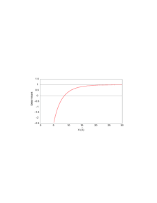
Figure 3: Determinant for the two-strand case with $a=2$.

4 Numerical Study of the Interaction Energy

Our strategy is to study the energy of configurations of DNA strands that capture as much as possible the symmetry of arrangements encountered in real aggregates [6]. The first case considered is of course that of the two-strand interaction. When then proceed to the many-body interactions with the strands sitting at the sites of hexagonal lattices like that of Fig. 1 which is for the maximum number of strands we were able to consider, i.e. 19 strands. We also present here results for four DNA strands sitting at the vertices of a rhombus. Thus the $x$-dependance of ${\cal E}(x)$ is that of the energy on the lattice spacing and making $x$ bigger or smaller means to expand or shrink the aggregate size, respectively. Of course, for big enough $x$ the situation one is describing is that of a dilute solution of DNA molecules, which is our starting point. The idealization here consist in the demanding a symmetry of arrangement even in the dilute phase.

To render the expression (3.40) suitable for such a study we first numerically perform the integral over $E$ and then plot the resulting expression ${\cal E}(x)$ where

$${\cal E}(x)=\frac{1}{8\pi}\ln\left(\det\gamma_{ij}(x)\right)\;,$$ (4.42)

and

$$\gamma_{ij}(x) = \delta_{ij}-\frac{K_{0}(\mu\;c_{ij}x)}{\ln(\mu/M)}(1-\delta_{ij})$$ (4.43)

$$= \delta_{ij}-aK_{0}(c_{ij}x)(1-\delta_{ij})\;.$$ (4.44)

The relative distances $l_{ij}=c_{ij}x$ are expressed in terms of the basic lattice distance $x$ and the numerical coefficients $c_{ij}$ take the symmetry of the given arrangement into account. In (4.44) we make explicit the choice $\mu=1$ (i.e. the distances are measured in units of $\mu^{-1}$). The other scale $M$ is constrained to be positive and less than $\mu(=1)$ and we write it as $0<M=e^{-1/a}<1$. In this fashion the range of $\cal E$ scales with $a$ and we present here results for $a=1$ and $a=2$.

The two-strand interaction energy is shown in Fig. 2. It is clearly attractive and finite-range. Similar attractive behaviors for the two-body interaction have been found in various models [7, 13]. What we observe here is that in those models it is not clear why the interaction still needs to be attractive for more than two strands. For the Casimir energy we shall soon see that this is indeed the case, since this attraction mechanism does not suffer of any frustration.

To establish whether the magnitude and range of this attractive energy is indeed relevant for the case of DNA aggregates we need to move, as said, to the many-body case. Before doing so we need to first consider that the distances are measured in units of $1/\mu\sim{\cal O}(10)$ Å. This gives a range of attraction that can be adjusted by fixing the free parameter $a$ to fit the typical distances reached within the aggregates. For the hexagonally packed toroidal condensates such distances range between [6] 18 Å and 28 Å, values clearly compatible with the range we obtain for the many-body interaction (see later).

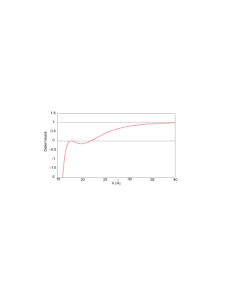
Figure 4: Determinant for the 19-strand case with $a=2$. Note that only the value $\bar{x}\sim 22$Å is the one to consider as the singular point.

To compare this quantum energy with thermal energy we write the integral in Eq.(3.40) in a dimensionless fashion so that the factor in front is $\hbar c\mu^{2}\sim 5\times 10$ eV/Å, where $c\sim 10^{8}ms^{-1}$. Hence, as the values of the integrals we obtain are ${\cal O}(10^{-3})$, the unit for the energy per length (in Å) is estimated to be ${\cal E}\sim 5\times 10^{-2}$ eV/Å. Thermal fluctuations, as computed for instance in [13], give for the two-body interaction a maximum value of ${\cal E}\sim 5\times 10^{-3}$ eV/Å at a separation distance of 10 Å. At this distance our interaction for the two-body case gives $5\times 10^{-2}$ eV/Å (for $a=1$) and $2\times 10^{-1}$ eV/Å (for $a=2$), i.e. a result that is between one and two orders of magnitude stronger. For the many-body case, the case of importance for the aggregates, this factor grows enormously but we cannot trust our approximations for $x$ too close to the singular value of the logarithm, say $\bar{x}$. It is clear, though, that at the distances of relevance this quantum energy is stronger (or much stronger) than thermal energy.

Let us look more closely to the singularity of the energy. We are able to numerically evaluate this $\bar{x}$ for the various cases by plotting the determinant that of course shows no such singularity as can be seen in Fig. 3 ($\bar{x}\sim 8$Å) and Fig. 4 ($\bar{x}\sim 22$Å) for the two-strand case and for the 19-strand case of Fig. 1, respectively. That singularity means that if only the Casimir force were present the strands would collapse to zero separation, an instance that does not occur in the real case because of other forces (not considered here) such as the electrostatic force that for more than two strands will give a net repulsive effect. Another important factor at such short distances is of course the finite size of DNA strands that have a transverse length (radius of the cylinder) of $10$Å. We take the distance $\bar{x}$ as the limit of validity of our approximations.

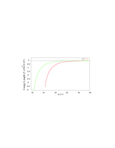
Figure 5: Interaction energy for the four-strand-rhombic case with $a=1$ (upper curve) and $a=2$ (lower curve). Distances $x$ are measured in units of $1/\mu\sim$ ${\cal O}(10)$ Å, while lineal energy density units are estimated to be $5\times 10^{-2}$ eV/Å.

Having established the above we have computed the energy for several interacting strands having various configurations. We present in Fig. 5 and in Fig.6 the results for four strands sitting at the vertices of a rhombus and for 19 strands arranged as in Fig. 1, respectively. Comparing these plots with that of the two strands interaction we clearly see that the attraction becomes stronger and acts on a larger range when the number of strands increases.

In the real case of aggregates it is always several DNA strands that interact, the two strands being only an idealization. Thus the fact that for 19 strands we find that (for $a=2$) the range of the force is in agreement with the typical values reported for DNA aggregates [6] we take it as an indication of the validity of our hypothesis that the quantum Casimir energy could hold together the aggregates. Furthermore, this force is many-body in nature and the many-body effects are big, another reason for taking the two-body interaction only as an indication of the real phenomenon.

That the many body effects are strong we proved in our numerical calculations where we compared the $N$-body energy of Eq. (4.42) with that obtained by summing up $(N/2)(N-1)$ two-body interactions. The results for four and seven strands are shown in Fig. 7 and Fig. 8, respectively, and they indicate that the effect grows with $N$.

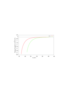
Figure 6: Interaction energy for the hexagonal lattice 19-strand configuration of Fig. 1 with $a=1$ (upper curve) and $a=2$ (lower curve). Distances $x$ are measured in units of $1/\mu\sim$ ${\cal O}(10)$ Å, while lineal energy density units are estimated to be $5\times 10^{-2}$ eV/Å.

5 Conclusions

The main result of this paper is to hint at quantum relativistic effects as viable candidates for the collapse of DNA strands into aggregates (after the OM condensation has taken place) and for holding them together into stable condensates. Rather than approaching the problem by setting-up from scratch a model based on quantum electrodynamics we built-up an effective model based on the classical PB equation of electrostatics and included the DNA strands (modeled here as infinite lines or delta functions) in the Boltzmann distribution, an instance that lead to a modified PB equation. The time-dependent fluctuations we then studied are quantum in nature, propagate at the speed of light in the medium and give rise to a Casimir force that we studied in various settings. In particular, we focused our attention on the difficult problem of computing such interaction for several DNA strands and were able to overcome the analytical challenges with numerical calculations performed for a variety of cases, most of which with hexagonal symmetry of arrangement (the typical situation reported in experiments).

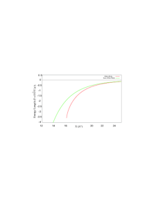
Figure 7: The lower curve is the interaction energy for the four-strand-rhombic configuration (many-body). The upper curve is what is obtained by summing-up the 6 two-body interactions. In both cases $a=2$. Distances $x$ are measured in units of $1/\mu\sim$ ${\cal O}(10)$ Å, while lineal energy density units are estimated to be $5\times 10^{-2}$ eV/Å.

The numerical calculations show many interesting features: the interaction is attractive and short range for the two-body case and is many-body, the departures from the “sum of two-bodies” being important and growing with the number of strands; the distance at which our approximations stop working is also obtained as the value at which the determinant function vanishes; finally, the magnitude and range of the interaction is such that it could explain the formation and stability of DNA aggregates, as a preliminary comparison with reported data shows.

Our model is a primitive one and to make full contact with experiments we propose it as one part of the puzzle as it needs to be seen as one of the concurrence of three mechanisms: (i) the zero-point quantum interaction, that gives the universal attraction (“glue”); (ii) the “frustrated force”, that takes into account the detailed structure (finite size and helical architecture) and the active role of counterions (these alone seem to reproduce the helical architecture [17]; (iii) water-related forces, that need to be included. That the interaction (3.40) alone does not give the full picture is seen from the singularity at a value $\bar{x}$ such that the determinant becomes zero. If only this force were present the DNA-cation complexes would collapse to zero separation, but at very short distances we should include nonlinear corrections to this force itself, and, even leaving aside water-related forces, at short distances the Wigner crystal effects should become important. Our goal here was to single-out the role of the zero-point quantum vacuum energy and we have shown that it is quite plausible that it plays a key role in the onset of the formation and in the follow-up stability of DNA aggregates.

It is pleasant to see that quantum effects might be essential for understanding an important biological problem (other quantum effects are important for enzyme catalysis [27] or speculated to be important for neural activity [28]) as this might serve as a solid basis for a more general understanding of the role of quantum mechanics for life [29].

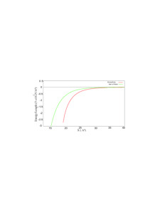
Figure 8: The lower curve is the interaction energy for the 7-strand configuration, i.e. for 7 strands sitting at the vertices and at the certer of a regular hexagon (many-body). The upper curve is what is obtained by summing-up the 21 two-body interactions. In both cases $a=2$. Distances $x$ are measured in units of $1/\mu\sim$ ${\cal O}(10)$ Å, while lineal energy density units are estimated to be $5\times 10^{-2}$ eV/Å.

References

- [1] W. M. Gelbart, R. F. Bruinsma, P. A. Pincus, V. A. Parsegian, Phys. Today 53 (2000) 38.
- [2] F. Oosawa, Biopolymers 6 (1968) 1633.
- [3] G. S. Manning, J. Chem. Phys. 51 (1969) 924.
- [4] Y. Levin, Rept. Prog. Phys. 65 (2002) 1577 [arXiv:cond-mat/0207086].
- [5] A. Yu. Grosberg, T. T. Nguyen, B. I. Shklovskii, Rev. Mod. Phys. 74 (2002) 329.
- [6] N. V. Hud, I. D. Vilfan, Annu. Rev. Biophys. Biomol. Struct. 34 (2005) 295.
- [7] A. A. Kornyshev, S. Leikin, Phys. Rev. Lett. 82 (1999) 4138.
- [8] A. A. Kornyshev, D. J. Lee, S. Leikin, A. Wynveen, Rev. Mod. Phys. 79 (2007) 943.
- [9] X. Qiu, K. Andresen, L. W. Kwok, J. S. Lamb, H. Y. Park, L. Pollack, Phys. Rev. Lett. 99 (2007) 038104.
- [10] H. M. Harreis, C. N. Likos, H. Löwen, Biophys. J. 84 (2003) 3607.
- [11] A. G. Cherstvy, A. A. Kornyshev, S. Leikin, J. Phys. Chem. B 106 (2002) 13362; A. G. Cherstvy, J. Phys.: Condens. Matter 17 (2005) 1363.
- [12] F. Oosawa, Polyelectrolytes, Dekker (New York) 1971.
- [13] N. Grønbech-Jensen, R. J. Mashl, R. F. Bruinsma, W. M. Gelbart Phys. Rev. Lett. 78 (1997) 2477.
- [14] B.-Y. Ha, A. Liu, Phys. Rev. Lett. 79 (1997) 1289.
- [15] R. Podgornik, V. A. Parsegian, Phys. Rev. Lett. 80 (1998) 1560.
- [16] A. Iorio, S. Sen, S. Sen, Do quantum effects hold together DNA condensates?, Int. J. Mod. Phys. B (2009) (to appear).
- [17] G. M. Grason, R. F. Bruinsma, Phys. Rev. Lett. 97 (2006) 027802; Phys. Rev. E 76 (2007) 021924.
- [18] R. Jackiw, in M. Beg Memorial Volume, A. Ali, P. Hoodboy Eds, World Scientific (Singapore) 1991.
- [19] V. A. Parsegian, Van Der Waals Forces, Cambridge Univ. Press (Cambridge) 2006.
- [20] V. V. Nesterenko, G. Lambiase and G. Scarpetta, Riv. Nuovo Cim. 27N6 (2004) 1.
- [21] B. W. Ninham, V. A. Parsegian, Biophys. J. 10 (1970) 646.
- [22] A. Scardicchio, Phys. Rev. D 72 (2005) 065004.
- [23] S. Albeverio, S. Gesztesy, R. Hoegh-Krohn, H. Holden, Solvable Models in Quantum Mechanics, AMS Chelsea Publishing, 2000.
- [24] R. P. Feynman, A. Hibbs, Quantum Mechanics and Path Integrals, McGraw Hill (New York) 1965.
- [25] P. Ramond, Field Theory: a modern primer, Addison-Wesley (Reading, Massachusetts) 1989.
- [26] R. L. Jaffe and A. Scardicchio, JHEP 0506 (2005) 006.
- [27] M. Garcia-Viloca, J. Gao, M. Karplus, D. G. Truhlar, Science 303 (2004) 186.
- [28] R. Penrose, The emperor’s new mind, Oxford Univ. Press (Oxford) 1989.
- [29] E. Schrödinger, What is life, Cambridge Univ. Press (Cambridge) 1944; H. Frölich, Phys. Lett. A 51 (1975) 21.