Dynamics of Entanglement and ‘Attractor’ states in The Tavis-Cummings Model

Abstract

We study the time evolution of $N_{q}$ two-level atoms (or qubits) interacting with a single mode of the quantised radiation field. In the case of two qubits, we show that for a set of initial conditions the reduced density matrix of the atomic system approaches that of a pure state at ${\textstyle\frac{t_{r}}{4}}$, halfway between that start of the collapse and the first mini revival peak, where $t_{r}$ is the time of the main revival. The pure state approached is the same for a set of initial conditions and is thus termed an ‘attractor state’. The set itself is termed the basin of attraction and the features are at the center of our attention. Extending to more qubits, we find that attractors are a generic feature of the multi qubit Jaynes Cummings model (JCM) and we therefore generalise the discovery by Gea-Banacloche for the one qubit case. We give the ‘basin of attraction’ for $N_{q}$ qubits and discuss the implications of the ‘attractor’ state in terms of the dynamics of $N_{q}$-body entanglement. We observe both collapse and revival and sudden birth/death of entanglement depending on the initial conditions.

I Introduction

The dynamics of two level quantum systems (also known as qubits) such as spins in a magnetic field, Rydberg atoms or superconducting qubits, coupled to a single mode of an electromagnetic cavity are of considerable interest in connection with NMR studies of atomic nuclei C. P. Slichter (1978), cavity quantum electrodynamics P. R. Berman (1994) and the physics of quantum computing M. A. Nielsen and I. L. Chuang (2001). The simplest model that captures the salient features of the physics in these fields is the Jaynes-Cummings model (JCM) E. T. Jaynes and F. W. Cummings (1963), which deals with only one qubit and its generalisation by Tavis and Cummings to the case of multiple qubits M. Tavis and F. W. Cummings (1968).

These models have many interesting features B. W. Shore and P. L. Knight (1993), but perhaps the most surprising prediction is the phenomena of ‘collapse and revival’ of the Rabi oscillations in the qubit system when the field is started in a coherent state ${\left|\alpha\right\rangle}$ C. C. Gerry and P. L. Knight (2005),

$${\left|\alpha\right\rangle}=e^{-{\left|\alpha\right|}^{2}/2}\sum_{n=0}^{\infty}\frac{\alpha^{n}}{\sqrt{n!}}{\left|n\right\rangle},\ \ \ \ \ \ \alpha={\left|\alpha\right|}e^{-i\theta}\;.$$ (1)

Here the state ${\left|n\right\rangle}$ is the eigenstate of the photon number operator $\hat{n}=a^{\dagger}a$ with eigenvalue $n$ and $\theta$ is the initial phase of the radiation field. ${\left|\alpha\right|}$ determines the size of the field, with $\bar{n}={\left\langle\alpha\right|}\hat{n}{\left|\alpha\right\rangle}=|\alpha|^{2}$.

In short what is found is that the initial Rabi-oscillations of the probability of being in a given qubit state decay on a time scale called the collapse time, $t_{c}$, but then revive after a much longer time, $t_{r}$, due to the quantum ‘graininess’ of the radiation field Cummings (1965); S. Barnett and P. Radmore (1997); J. H. Eberly, N. B. Narozhny, J. J. Sanchez-Mongragon (1980). Whilst the nature of this remarkable phenomenon in the case of one qubit is now well understood B. W. Shore and P. L. Knight (1993), both experimentally P. R. Berman (1994) and theoretically H. I. Yoo and J. H. Eberly (1985), the multi qubit case M. Tavis and F. W. Cummings (1968); M. Ueda, T. Wakabayashi, and M. Kuwata-Gonokami (1996) has not been explored to the same extent. For instance, the occurrence between $t_{c}$ and $t_{r}$, of what we shall call the ‘attractor’ state has only been fully investigated in the one qubit limit. This intriguing aspect of quantum dynamics was discovered and highlighted by Gea-Banacloche J. Gea-Banacloche (1990, 1991) in his study of the one qubit case. In this paper we report on our investigation of analogous ‘attractors’ in cases of more than one qubit.

The organization of this paper is as follows. In Sec. II, the dynamics of the resonant JCM (single qubit coupled to a cavity system) is presented. This sets up our notation, analytic tools and methods of data presentation. In Sec. III we extend the model to two qubits and show that the idea of an ‘attractor’ state still exists. We investigate the dynamics in depth and quantify the set of initial states that approach the ‘attractor’, giving the ‘basin of attraction’. We show that the atomic system exhibits interesting entanglement properties, in particular that the entanglement can vanish and then return at a later time. Furthermore, the manner in which this occurs depends on whether we are in or outside this basin of attraction. In Sec. IV we develop these ideas further from those of the two-qubit case and find a set of initial states (the basin of attraction) from which the system always goes to the ‘attractor’ state for an arbitrary number of qubits. In the limit of large qubit number we rewrite our qubit equations in terms of spin coherent states and demonstrate some intriguing phenomena associated with the $N_{q}$-qubit JCM, especially the collapse and revival of $N_{q}$-body entanglement. Whilst our method of analysis, and some of our results, are similar to those of Chumakov et al. S. M. Chumakov, A. B. Klimov and J. J. Sanchez-Mondragon (1994) and Meunier et al. T. Meunier, A. Le Diffon, C. Ruef, P. Degiovanni and J.-M. Raimond (2006), our focus is on the quantum information aspects of the problem and in particular the dynamics of entanglement.

II Features of the Jaynes-Cummings Model

We first review the JCM and appearance of ‘attractor’ states in the one qubit case E. Schrödinger (1935); V. Bužek, H. Moya-Cessa, P. L. Knight and S. J. D. Phoenix (1992); P. L. Knight and B. W. Shore (1993). The JCM model consists of a single qubit coupled to a single mode of a quantised electromagnetic field. The two possible states of the qubit are the ground state ${\left|g\right\rangle}$, with energy $\epsilon_{g}$, or its excited state ${\left|e\right\rangle}$, with energy $\epsilon_{e}$. We consider the following Hamiltonian:

$$\hat{H} = \hbar\omega\hat{a}^{{\dagger}}\hat{a}+\frac{\hbar\Omega}{2}\hat{\sigma}^{z}+\hbar\lambda\left(\hat{a}\hat{\sigma}^{+}+\hat{a}^{{\dagger}}\hat{\sigma}^{-}\right)$$ (2)

$$\hat{\sigma}^{z} = {\left|e\right\rangle}{\left\langle e\right|}-{\left|g\right\rangle}{\left\langle g\right|},\ \hat{\sigma}^{+}={\left|e\right\rangle}{\left\langle g\right|},\ \hat{\sigma}^{-}={\left|g\right\rangle}{\left\langle e\right|}$$ (3)

where $\hat{a}^{{\dagger}}$ and $\hat{a}$ are the creation and annihilation operators of photons with frequency $\omega$, $\hbar\Omega=\epsilon_{e}-\epsilon_{g}$ and $\lambda$ the cavity-qubit coupling constant. The model is only valid close to resonance and we shall only consider the resonant case of $\omega=\Omega$.

We have an initial state:

$${\left|\Psi_{1}(t=0)\right\rangle}={\left|\psi_{1}\right\rangle}{\left|\alpha\right\rangle}=(C_{g}{\left|g\right\rangle}+C_{e}{\left|e\right\rangle})\sum_{n=0}^{\infty}C_{n}{\left|n\right\rangle},$$ (4)

where the state of the qubit is normalised so ${\left|C_{e}\right|}^{2}+{\left|C_{g}\right|}^{2}=1$ and the field is started in a coherent state. In the interaction picture (i.e. in a rotating reference frame) we obtain a solution to the Hamiltonian:

$${\left|\Psi_{1}(t)\right\rangle} = \sum_{n=0}^{\infty}\left[\left(C_{e}C_{n}\cos\left(\lambda\sqrt{n+1}t\right)-iC_{g}C_{n+1}\sin\left(\lambda\sqrt{n+1}t\right)\right){\left|e,n\right\rangle}\right.$$ (5)

$$\left.\left(C_{g}C_{n+1}\cos\left(\lambda\sqrt{n+1}t\right)-iC_{e}C_{n}\sin\left(\lambda\sqrt{n+1}t\right)\right){\left|g,n+1\right\rangle}\right]+C_{g}C_{0}{\left|g,0\right\rangle}.$$

In spite of its relative simplicity, Eq. (5) exhibits a wide range of interesting phenomena. A much studied example is the collapse and revival of Rabi oscillations. If the qubit is started in the ground state then initially the probability of the qubit being in the ground state oscillates from one to zero at the Rabi frequency. These oscillations then decay on a time scale called the collapse time, $t_{c}=\frac{2}{\lambda}$, but then revive after a much longer time:

$$t_{r}=\frac{2\pi\sqrt{\bar{n}}}{\lambda}.$$ (6)

When $\bar{n}\gg\lambda t$ we can approximate ${\left|\Psi_{1}(t)\right\rangle}$ in Eq. (5) by ${\left|\widetilde{\Psi}_{1}(t)\right\rangle}$:

$${\left|\widetilde{\Psi}_{1}(t)\right\rangle} = \beta_{+\frac{1}{2}}(t){\left|D_{+\frac{1}{2}}(t)\right\rangle}{\left|\Phi_{+\frac{1}{2}}(t)\right\rangle}+\beta_{-\frac{1}{2}}(t){\left|D_{-\frac{1}{2}}(t)\right\rangle}{\left|\Phi_{-\frac{1}{2}}(t)\right\rangle},$$ (7)

where $\beta_{\pm\frac{1}{2}}(t)$ is a normalisation factor, ${\left|D_{\pm\frac{1}{2}}(t)\right\rangle}$ is a state of the qubits and ${\left|\Phi_{\pm\frac{1}{2}}(t)\right\rangle}$ is a state of the field.

$$\beta_{\pm\frac{1}{2}}(t) = \frac{1}{\sqrt{2}}e^{\pm i\pi\frac{t}{t_{r}}\left(\bar{n}+1\right)}\left(e^{i\theta}C_{e}\mp C_{g}\right)$$ (8)

$${\left|D_{\pm\frac{1}{2}}(t)\right\rangle} = \frac{1}{\sqrt{2}}\left(e^{-i\theta}{\left|e\right\rangle}\mp e^{\mp i\pi t/t_{r}}{\left|g\right\rangle}\right)$$ (9)

$${\left|\Phi_{\pm\frac{1}{2}}(t)\right\rangle} = {\left|e^{\pm i\pi t/t_{r}}\alpha\right\rangle}.$$ (10)

With the solution written in this form it is clear there are two distinct parts to the wavefunction. In fact the field just consists of two different coherent states that are out of phase by $\lambda t/\sqrt{\bar{n}}$. In a penetrating study of this model Gea-Banacloche J. Gea-Banacloche (1991) noted that at a time ${\textstyle\frac{t_{r}}{2}}$, in the very large $\bar{n}$ approximation, the qubit disentangles itself completely from the field and the wavefunction factors into a product state of the radiation field and the qubit.

To make this more apparent we rewrite Eq. (8) – Eq. (10) at the time $t={\textstyle\frac{t_{r}}{2}}$.

$$\beta_{\pm\frac{1}{2}}({\textstyle\frac{t_{r}}{2}}) = \pm\frac{i}{\sqrt{2}}e^{\pm i\pi\bar{n}/2}\left(e^{i\theta}C_{e}\mp C_{g}\right)$$ (11)

$${\left|D_{\pm\frac{1}{2}}({\textstyle\frac{t_{r}}{2}})\right\rangle} = \frac{1}{\sqrt{2}}\left(e^{-i\theta}{\left|e\right\rangle}+i{\left|g\right\rangle}\right)$$ (12)

$${\left|\Phi_{\pm\frac{1}{2}}({\textstyle\frac{t_{r}}{2}})\right\rangle} = {\left|\pm i\alpha\right\rangle}.$$ (13)

With the wavefunction written in this way it can be seen that the two states ${\left|D_{+\frac{1}{2}}({\textstyle\frac{t_{r}}{2}})\right\rangle}$ and ${\left|D_{-\frac{1}{2}}({\textstyle\frac{t_{r}}{2}})\right\rangle}$ are in fact the same at the time ${\textstyle\frac{t_{r}}{2}}$. We label this state ${\left|\psi_{1\,att}^{+}\right\rangle}$:

$${\left|\psi_{1\,att}^{\pm}\right\rangle}=\frac{1}{\sqrt{2}}\left(e^{-i\theta}{\left|e\right\rangle}\pm i{\left|g\right\rangle}\right)\;.$$ (14)

This state is independent of the initial coefficients $C_{e}$ and $C_{g}$ and only depends on the phase $\theta$ of the initial coherent state, Eq. (1). Throughout this paper we follow Phoenix and Knight S. J. D Phoenix and P. L. Knight (1991) and call this state an ‘attractor’ state. Note that we use the term ‘attractor’ to refer to ${\left|\psi^{\pm}_{1\,att}\right\rangle}$ even though in the theory of non-linear differential equations the term attractor is reserved for solutions which, when reached, after evolving from an arbitrary initial condition, stop changing with time. As a consequence the qubit state can be factorised out of the wavefunction meaning the qubit and the field are in a product state:

$${\left|\widetilde{\Psi}_{1}({\textstyle\frac{t_{r}}{2}})\right\rangle} = \frac{{\left|\psi_{1\,att}^{+}\right\rangle}}{\sqrt{2}}\left(ie^{i\pi\bar{n}/2}\left(e^{i\theta}C_{e}-C_{g}\right){\left|i\alpha\right\rangle}-ie^{-i\pi\bar{n}/2}\left(e^{i\theta}C_{e}+C_{g}\right){\left|-i\alpha\right\rangle}\right).$$ (15)

It is clear that all the information of the initial state about the qubit is stored in the radiation field which happens to be in a “Schrödinger cat” state. At a later time $t=\frac{3t_{r}}{2}$, the qubit again disentangles itself completely from the field and goes to a pure state. The qubit state at this time is orthogonal to ${\left|\psi_{1\,att}^{+}\right\rangle}$ and we label it ${\left|\psi_{1\,att}^{-}\right\rangle}$. This remarkable behaviour is most unlike the consequences of a linear Schrödinger equation satisfied by a qubit without the cavity field or with a classical field and, as was stressed by Gea-Banacloche, is a natural route to quantum state preparation. All initial qubit states tend to the same ‘attractor’ state (which is determined by the initial phase of the field state) and the quantum information about the initial qubit state has effectively been swapped out and encoded into the field at the ‘attractor times’.

Before we move on to describe the results of numerical simulations we consider the field, Eq. (10), at two revival times $t=t_{r}$ and $t=2t_{r}$. At both these times the field states ${\left|\Phi_{\pm\frac{1}{2}}(t)\right\rangle}$ become equal, with ${\left|\Phi_{+\frac{1}{2}}(t_{r})\right\rangle}={\left|\Phi_{-\frac{1}{2}}(t_{r})\right\rangle}={\left|-\alpha\right\rangle}$ and ${\left|\Phi_{+\frac{1}{2}}(2t_{r})\right\rangle}={\left|\Phi_{-\frac{1}{2}}(2t_{r})\right\rangle}={\left|\alpha\right\rangle}$. As a consequence the system is once again in a product state as the field can be factorised out of the wavefunction for the whole state. The information about the initial state of the qubits has been transferred from the field back to the qubits.

By considering the average number of photons in the field, $\bar{n}$, to be large many interesting observations have been made of the JCM. It was shown that the system repeatedly evolves from a product state to an entangled state and back again. Although the analytical equations for large values of $\bar{n}$ clearly show this behaviour, we now consider the exact solution ${\left|\Psi_{1}(t)\right\rangle}$ for modest $\bar{n}$ ($\bar{n}=50$), shown in Eq. (5) and comment on the results of numerical simulations for the qubit and the photon sector separately.

We consider the state of the qubits after tracing out the field state. The probability of the qubits being in the state ${\left|g\right\rangle}$ is,

$$P_{1\,g}(t)={\left\langle g\right|}\rho_{q}(t){\left|g\right\rangle}=\sum_{n=0}^{\infty}{\left|{\left\langle g,n|\Psi_{1}(t)\right\rangle}\right|}^{2}$$ (16)

where $\rho_{q}(t)=\mathrm{Tr}_{f}\left({\left|\Psi_{1}(t)\right\rangle}{\left\langle\Psi_{1}(t)\right|}\right)$ is the reduced density matrix at a certain time for the qubits when the field has been traced out. Throughout this paper all instances of the letter $q$ refer to the qubit system and $f$ refers to the field. The results are depicted in Fig. 1 for the initial state ${\left|\Psi_{1}(t=0)\right\rangle}={\left|g\right\rangle}{\left|\alpha\right\rangle}$ and the well known phenomenon of collapse and revival can be seen. For numerical reasons the sum over $n$ is truncated at $n_{max}=200$ as this is adequate for the average number of photons in the mode of $\bar{n}=50$.

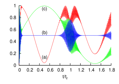
Figure 1: (color online) Time evolution for a system with one qubit when the qubit starts in the initial state ${\left|g\right\rangle}$ and the value of $\bar{n}=50$. (a) the entropy of the qubit. (b) the probability of being in the qubit’s initial state ${\left|g\right\rangle}$. (c) the probability of being in the state ${\left|\psi_{att}^{+}\right\rangle}$. At ${\textstyle\frac{t_{r}}{2}}$ the probability of being in the ‘attractor’ state goes to one while the entropy goes to zero.

An entropy measurement of the system can be made at any point in time. Entropy is a well defined quantity that measures the disorder of a system and the purity of a quantum state. In cases where the time-dependent Schrödinger equation (as opposed to some master equation for reduced dynamics) determines the time evolution of a system, the value of the entropy remains constant. The complete systems (qubits plus field) we study are always started in a pure state and follow Schrödinger dynamics; therefore the entropy of the complete systems always remains zero as we have a pure state. In these systems the individual entropies, of the qubits or the field, are of more interest. We calculate the partial entropy from the reduced density matrix $\rho_{q}$ using the rescaled von Neumann entropy J. von Neumann (1955); A. Wehrl (1978),

$$S_{q}(t)=-\mathrm{Tr}(\rho_{q}(t)\mathrm{log_{2}}\rho_{q}(t))/N_{q},$$ (17)

which is rescaled such that the entropy of the qubits ranges from zero, for a pure state, to one, for a maximally mixed state. For the bipartite case (the one qubit $N_{q}=1$ JCM) this reduces to the standard von Neumann entropy. As was discovered by Araki and Lieb H. Araki and E. Lieb (1970), if the system is started in a pure state then $S_{q}(t)$=$S_{f}(t)$ for all time, where $S_{f}(t)$ is the entropy of the field system calculated from reduced density matrix $\rho_{f}(t)=\mathrm{Tr}_{q}\left({\left|\Psi_{1}(t)\right\rangle}{\left\langle\Psi_{1}(t)\right|}\right)$. Therefore for the rest of the paper we shall refer to the value of $S_{q}(t)$ only when we mention entropy.

In quantum information these partial entropies provide a measure of the entanglement present between the two systems, known as the entropy of entanglement V. Vedral, M. B. Plenio, K. Jacobs, and P. L. Knight (1997); W. J. Munro, D. F. V. James, A. G. White, and P. G. Kwiat (2001). If the entropy is zero then the state being measured is pure and there is no entanglement present. If the value of the entropy is non zero then there is some entanglement present between the two parts of the system and the reduced density matrix is mixed. Returning to the JCM we note that the ‘attractor’ state, Eq. (14), is a pure state and hence the value $S_{q}({\textstyle\frac{t_{r}}{2}})$ will be zero. So the qubit has disentangled itself from the field and there is no entanglement present at this time. The reduced entropy is a powerful tool in understanding entanglement in the JCM and it is worthwhile recalling an example of its power to elucidate the quantum dynamics S. J. D Pheonix and P. L. Knight (1988); S. J. D Phoenix and P. L. Knight (1991).

We have numerically evaluated $S_{q}$ for qubits started in the initial state ${\left|\Psi_{1}(t=0)\right\rangle}={\left|g\right\rangle}{\left|\alpha\right\rangle}$ using the exact solution for ${\left|\Psi_{1}(t)\right\rangle}$ and the results are shown in Fig. 1 by the curve labelled (a). We also plot the probability $P_{1\,att}(t)={\left\langle\psi^{+}_{1\,att}\right|}\rho_{q}(t){\left|\psi^{+}_{1\,att}\right\rangle}$ that the qubit is in the ‘attractor’ state ${\left|\psi_{1\,att}^{+}\right\rangle}$, as defined in Eq. (14), shown by the curve labelled (c).

Evidently at the time ${\textstyle\frac{t_{r}}{2}}$ the reduced entropy goes very close to zero and $P_{1\,att}({\textstyle\frac{t_{r}}{2}})$ goes very close to one. As mentioned above, this means there is very little field-qubit entanglement present and the qubit is essentially in the ‘attractor’ state, ${\left|\psi_{1\,att}^{+}\right\rangle}$, as defined in Eq. (14). At $\frac{3t_{r}}{2}$ the probability of being in this ‘attractor’ state approaches zero, as the qubit is in the state ${\left|\psi_{1\,att}^{-}\right\rangle}$, which is orthogonal to ${\left|\psi_{1\,att}^{+}\right\rangle}$. These results all agree with the discussions of Eq. (15). At future ‘attractor’ times the system alternates between ${\left|\psi_{1\,att}^{+}\right\rangle}$ and ${\left|\psi_{1\,att}^{-}\right\rangle}$.

A big difference between numerical results and the large $\bar{n}$ solution is noticed at the time $t=t_{r}$. Earlier we showed that the solution in the large $\bar{n}$ approximation will return to a pure state at this time, but in Fig. 1 the entropy has a large value of $0.7$, wedged between two maxima (indicating large entanglement between qubit and field). This is because the width of this dip is on a time scale similar to the collapse time, much narrower than the entropy dip at ${\textstyle\frac{t_{r}}{2}}$. As the value of $\bar{n}$ is increased in numerical simulations, the value of the entropy at $t=t_{r}$ gets closer to zero, but we see that even for fairly large coherent states, the large $\bar{n}$ approximation can deviate significantly from the full solution.

So far we have reviewed the time evolution of the reduced qubit density matrix in the one-qubit and one mode system. Before we move on to address the two-qubit case we calculate the $Q$ function C. W. Gardiner and P. Zoller (1991) to investigate the radiation field,

$$Q(\alpha,t)={\left\langle\alpha\right|}\rho_{f}(t){\left|\alpha\right\rangle}.$$ (18)

This is shown in Fig. 2 in the rotating reference frame for the exact solution as contour plots. We give an example of a 3d plot of Fig. 2(b) in Fig. 3, but for the rest of the paper we will use the 2D contour plots.

Figure 2: (color online) A contour plot of the $Q$ function at six different times when the qubit is in the initial state ${\left|g\right\rangle}$ and $\bar{n}=50$. The atomic dipole states are represented by arrows. (a) the time $t=0$. The system is started in a coherent state which is shown by a circle of uncertainty in phase space. (b) a time a little after that of figure (a), $t={\textstyle\frac{t_{r}}{8}}$. The ‘blobs’ are well separated and are moving around a circle of fixed radius. (c) the time $t={\textstyle\frac{t_{r}}{2}}$. This corresponds to the first dip in entropy. (d) just before the time $t=t_{r}$. This is just before the revival time and the two ‘blobs’ will overlap. (e) the time ${\textstyle\frac{3t_{r}}{2}}$. The second dip in the entropy. (f) the time $t=2t_{r}$. Both the wavepackets have returned to their original position.

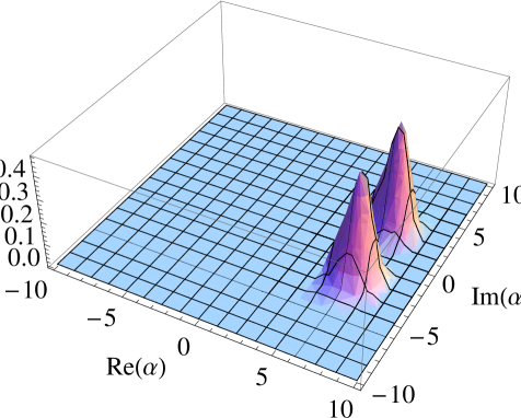
Figure 3: (color online) The $Q$ function in 3D for the time $t={\textstyle\frac{t_{r}}{8}}$ corresponding to diagram (b) in Fig. (2). We notice two distinct peaks of equal height that are very similar to coherent states.

The $Q$ function shows a set of two wavepackets of the cavity field, each of which can be thought of as a Gea-Banacloche state J. Gea-Banacloche (1991) in the large $\bar{n}$ solution. As a function of time the two ‘blobs’ move around the complex plane and follow the circular path of radius $\sqrt{\bar{n}}$. These ‘blobs’ start to smear out and become distorted from the original coherent state. Although the wavepackets all begin in the same place, they evolve with different frequencies, so the states begin to separate. After a period of time, depending on the differences between the frequencies, the different ‘blobs’ are separated by more than their diameter and can be easily distinguished. Eventually these two wavepackets will again overlap and this occurs at the revival time, $t=t_{r}$. When these ’blobs’ have some overlap in phase space there will be Rabi oscillations in the qubit probability, giving the periodic sequence of revivals seen in Fig. 1. However, as can be seen in Fig. 2(d), at the revival time, $t_{r}$, the ’blobs’ have undergone some distortion and so the wave packets are no longer simple coherent states. This distortion elongates the wave packets, and so they overlap for a longer time than in the ideal coherent state case. We therefore understand the lack of a full amplitude revival, $P_{1g}(t_{r})=1$, as due to the spreading, and hence distinguishability, of the field states. When the value of $\bar{n}$ gets very large there is less distortion and the Gea-Banacloche states stay exact coherent states throughout their evolution.

Also included in Fig. 2 is an arrow for each ‘blob’ which represents the average atomic polarisation, $\overrightarrow{d_{\pm\frac{1}{2}}}(t)={\left\langle D_{\pm\frac{1}{2}}(t)\right|}\overrightarrow{\hat{\sigma}}{\left|D_{\pm\frac{1}{2}}(t)\right\rangle}$ in the equatorial plane of the Bloch sphere. Fig. 2(c) shows the two dipole arrows are in line and pointing in the same direction at the time ${\textstyle\frac{t_{r}}{2}}$ because ${\left|D_{+\frac{1}{2}}({\textstyle\frac{t_{r}}{2}})\right\rangle}={\left|D_{-\frac{1}{2}}({\textstyle\frac{t_{r}}{2}})\right\rangle}={\left|\psi_{1\,att}^{+}\right\rangle}$. The arrows in Fig. 2(e) are again both the same, but are pointing in a different direction as ${\left|D_{+\frac{1}{2}}(\frac{3t_{r}}{2})\right\rangle}={\left|D_{-\frac{1}{2}}(\frac{3t_{r}}{2})\right\rangle}={\left|\psi_{1\,att}^{-}\right\rangle}$. The field states are moving in a different direction in Fig. 2(e) to that of Fig. 2(c) and their identity has swapped. These arrows can be used to see if the two qubit states are the same and the direction of the dipole arrows highlights we are in a different ‘attractor’ state.

Inspired by the above behaviour, in this paper we extend the analysis and investigate new problems. In particular we address the question: “Are there similar ‘attractor’ states in multi qubit systems and what are the implications of their existence?”

III Two Qubit Jaynes-Cummings Model

The $N_{q}$ qubit Hamiltonian, which in this section we treat for $N_{q}=2$ so $i=1,2$, is a generalisation of Eq. (2). It is called the Tavis-Cummings Hamiltonian M. Tavis and F. W. Cummings (1968):

$$\hat{H} = \hbar\omega\hat{a}^{{\dagger}}\hat{a}+\frac{\hbar}{2}\sum_{i=1}^{N_{q}}\Omega_{i}\hat{\sigma}_{i}^{z}+\hbar\sum_{i=1}^{N_{q}}\lambda_{i}\left(\hat{a}\hat{\sigma}_{i}^{+}+\hat{a}^{{\dagger}}\hat{\sigma}_{i}^{-}\right).$$ (19)

For brevity we only consider the solution for the case $\lambda_{1}=\lambda_{2}=\lambda$ and $\omega=\Omega_{1}=\Omega_{2}$. This model has been studied in detail by Chumakov et al. S. M. Chumakov, A. B. Klimov and J. J. Sanchez-Mondragon (1995) and the large $\bar{n}$ solution has been found S. M. Chumakov, A. B. Klimov and J. J. Sanchez-Mondragon (1994); T. Meunier, A. Le Diffon, C. Ruef, P. Degiovanni and J.-M. Raimond (2006) with similar results to our analysis. Adding another qubit to the system yields a more complex system which can exhibit interesting entanglement properties as not only can the two qubits be entangled with the field, but they can also be entangled between themselves.

We have investigated the evolution of the system over time, with analytical solutions in the large $\bar{n}$ approximation D. A. Rodrigues, C. E. A. Jarvis, B. L. Györffy, T. P. Spiller and J F Annett (2008) and the numerically evaluated exact solution. To summarise these we start with the initial state:

$${\left|\Psi_{2}(t=0)\right\rangle}={\left|\psi_{2}\right\rangle}{\left|\alpha\right\rangle}=\left(C_{ee}{\left|ee\right\rangle}+C_{eg}{\left|eg\right\rangle}+C_{ge}{\left|ge\right\rangle}+C_{gg}{\left|gg\right\rangle}\right){\left|\alpha\right\rangle},$$ (20)

where the state is normalised so ${\left|C_{ee}\right|}^{2}+{\left|C_{eg}\right|}^{2}+{\left|C_{ge}\right|}^{2}+{\left|C_{gg}\right|}^{2}=1$. Following the same procedure as in the one qubit case we solve the Hamiltonian and approximate for large $\bar{n}$. The time evolution of this state takes the following form:

$${\left|\widetilde{\Psi}_{2}(t)\right\rangle}=\sum^{1}_{k=-1}\beta_{k}(t){\left|D_{k}(t)\right\rangle}\otimes{\left|\Phi_{k}(t)\right\rangle},$$ (21)

where $k=-1,0$ or $1$ and:

$$\beta_{\pm 1}(t) = \frac{e^{\pm 2i\pi\frac{t}{t_{r}}\left(\bar{n}+2\right)}}{2}(e^{2i\theta}C_{ee}\mp e^{i\theta}(C_{eg}+C_{ge})+C_{gg}),$$ (22)

$$\beta_{0} = \frac{1}{\sqrt{2}}\sqrt{{\left|e^{2i\theta}C_{ee}-C_{gg}\right|}^{2}+{\left|C_{eg}-C_{ge}\right|}^{2}},$$ (23)

$${\left|D_{0}(t)\right\rangle} = {\left|D_{0}\right\rangle}=\frac{(e^{2i\theta}C_{ee}-C_{gg})(e^{-2i\theta}{\left|ee\right\rangle}-{\left|gg\right\rangle})+(C_{eg}-C_{ge})({\left|eg\right\rangle}-{\left|ge\right\rangle})}{\sqrt{2\left({\left|e^{2i\theta}C_{ee}-C_{gg}\right|}^{2}+{\left|C_{eg}-C_{ge}\right|}^{2}\right)}},$$ (24)

$${\left|D_{\pm 1}(t)\right\rangle} = \frac{1}{2}[e^{-2i\theta}{\left|ee\right\rangle}\mp e^{\mp 2i\pi t/t_{r}}e^{-i\theta}({\left|eg\right\rangle}+{\left|ge\right\rangle})+e^{\mp 4i\pi t/t_{r}}{\left|gg\right\rangle}],$$ (25)

$$= {\left|D_{\pm\frac{1}{2}}\left(2t\right)\right\rangle}\otimes{\left|D_{\pm\frac{1}{2}}\left(2t\right)\right\rangle},$$ (26)

$${\left|\Phi_{k}(t)\right\rangle} = {\left|e^{2ik\pi t/t_{r}}\alpha\right\rangle}.$$ (27)

Note that the state ${\left|D_{0}(t)\right\rangle}={\left|D_{0}\right\rangle}$ is time-independent and is thus a maximally entangled qubit state for all times if $C_{eg}=C_{ge}$ D. A. Rodrigues, C. E. A. Jarvis, B. L. Györffy, T. P. Spiller and J F Annett (2008). The field states are called Gea-Banacloche states and once again have a specific qubit state associated to each of them.

By making the observation shown in Eq. (26) it is easy to see that the two qubit states ${\left|D_{\pm 1}(t)\right\rangle}$ are direct products of the one qubit states ${\left|D_{\pm\frac{1}{2}}(t)\right\rangle}$ up to a mapping $t\rightarrow 2t$. This can be used to predict the behaviour of ${\left|D_{\pm 1}(t)\right\rangle}$. As stated in Sec. II ${\left|D_{\pm\frac{1}{2}}({\textstyle\frac{t_{r}}{2}})\right\rangle}={\left|\psi_{1\,att}^{+}\right\rangle}$ therefore we can conclude that ${\left|D_{\pm 1}(t)\right\rangle}$ will go to a direct product of ${\left|\psi_{1\,att}^{+}\right\rangle}$ at $t={\textstyle\frac{t_{r}}{4}}$.

$${\left|D_{\pm 1}({\textstyle\frac{t_{r}}{4}})\right\rangle} = {\left|D_{\pm\frac{1}{2}}\left({\textstyle\frac{t_{r}}{2}}\right)\right\rangle}\otimes{\left|D_{\pm\frac{1}{2}}\left({\textstyle\frac{t_{r}}{2}}\right)\right\rangle}$$ (28)

$$= {\left|\psi_{1\,att}^{+}\right\rangle}\otimes{\left|\psi_{1\,att}^{+}\right\rangle}$$ (29)

$$= {\left|\psi^{+}_{2\,att}\right\rangle}$$ (30)

So we have found a term that is similar to the one qubit ‘attractor’ state, ${\left|\psi_{1\,att}^{+}\right\rangle}$, which we shall label the two qubit ‘attractor’ state, ${\left|\psi_{2\,att}^{+}\right\rangle}$:

$${\left|\psi^{\pm}_{2\,att}\right\rangle}=\frac{1}{2}\left(e^{2i\theta}{\left|ee\right\rangle}\pm ie^{i\theta}\left({\left|eg\right\rangle}+{\left|ge\right\rangle}\right)-{\left|gg\right\rangle}\right)$$ (31)

In the one qubit case the qubit system went to a second ‘attractor’ state ${\left|\psi_{1\,att}^{-}\right\rangle}$ at the time $\frac{3t_{r}}{2}$ and means ${\left|D_{\pm 1}(\frac{3t_{r}}{4})\right\rangle}={\left|\psi_{1\,att}^{-}\right\rangle}\otimes{\left|\psi_{1\,att}^{-}\right\rangle}={\left|\psi^{-}_{2\,att}\right\rangle}$.

III.1 Basin of Attraction

The two qubit JCM is more complicated than the original one qubit case and shows some very interesting properties. Firstly we rewrite the wavefunction for the whole system as the time $t={\textstyle\frac{t_{r}}{4}}$ to understand the two qubit case in more detail.

$${\left|\widetilde{\Psi}_{2}({\textstyle\frac{t_{r}}{4}})\right\rangle} = -\frac{1}{2}{\left|\psi_{2\,att}^{+}\right\rangle}\left[\left(e^{2i\theta}C_{ee}+C_{gg}\right)\left(e^{i\pi\bar{n}/2}{\left|i\alpha\right\rangle}+e^{-i\pi\bar{n}/2}{\left|-i\alpha\right\rangle}\right)\right.$$ (32)

$$- \left.e^{i\theta}\left(C_{eg}+C_{ge}\right)\left(e^{i\pi\bar{n}/2}{\left|i\alpha\right\rangle}-e^{-i\pi\bar{n}/2}{\left|-i\alpha\right\rangle}\right)\right]+\beta_{0}{\left|D_{0}\right\rangle}{\left|\alpha\right\rangle}$$

With the wavefunction written in this form we can see which initial conditions result in the entropy going to zero. Indeed when $\beta_{0}=0$ the qubit and field parts are each in a product state, so there is no qubit-resonator entanglement present. There is also no qubit-qubit entanglement as these are in the unentangled ‘attractor’ state and this means there is absolutely no entanglement in the system at $t={\textstyle\frac{t_{r}}{4}}$. Interestingly, the information on the initial state of the qubits is again stored in the radiation field and the qubits are in a spin coherent ‘attractor’ state (see appendix A).

The initial conditions of the qubit that results in $\beta_{0}=0$ are: $e^{i\theta}C_{ee}=e^{-i\theta}C_{gg}=a$ and $C_{eg}=C_{ge}=\sqrt{\frac{1}{2}-{\left|a\right|}^{2}}$. So the initial state of the qubits will be of the form:

$${\left|\psi_{2}\right\rangle}=a(e^{-i\theta}{\left|ee\right\rangle}+e^{i\theta}{\left|gg\right\rangle})+\sqrt{\frac{1}{2}-{\left|a\right|}^{2}}({\left|eg\right\rangle}+{\left|ge\right\rangle})$$ (33)

where $\theta$ is the initial phase of the radiation field and $0\leq{\left|a\right|}\leq\frac{1}{\sqrt{2}}$. These states lie in the symmetric subspace and have some interesting properties that will be discussed in section III.2. While the qubit state is within this basin of attraction its state is parameterized by the single complex variable $a$ and the wavefunction only contains two field states, ${\left|\Phi_{\pm 1}(t)\right\rangle}$. At the time ${\textstyle\frac{t_{r}}{4}}$ these two field states are macroscopically distinct coherent states:

$${\left|\widetilde{\Psi}_{2}({\textstyle\frac{t_{r}}{4}})\right\rangle} = -e^{i\theta}{\left|\psi_{2\,att}^{+}\right\rangle}\left[e^{i\pi\bar{n}/2}\left(a-\sqrt{\frac{1}{2}-{\left|a\right|}^{2}}\right){\left|i\alpha\right\rangle}+e^{-i\pi\bar{n}/2}\left(a+\sqrt{\frac{1}{2}-{\left|a\right|}^{2}}\right){\left|-i\alpha\right\rangle}\right].$$

We now see that the initial state of the qubits alters the relative proportions of ${\left|\alpha\right\rangle}$ with respect to ${\left|-\alpha\right\rangle}$. This is also seen in the one qubit case and is the mechanism whereby the quantum information of the initial qubit state is encoded in the field. State preparation of a Schrödinger cat state utilizing this phenomenon has been discussed J. Gea-Banacloche (1991); B. Yurke and D. Stoler (1986). With the two qubit case the same protocol can be used, but is not so useful as the initial qubit state has to be within the basin of attraction in contrast to the one qubit case where all initial qubit states lead to a Schrödinger cat state at the ‘attractor’ times.

There is also a connection between the field states ${\left|\Phi_{\pm 1}(t)\right\rangle}$ in the two qubit case and the field states ${\left|\Phi_{\pm\frac{1}{2}}(t)\right\rangle}$ from the one qubit case, ${\left|\Phi_{\pm 1}(t)\right\rangle}={\left|\Phi_{\pm\frac{1}{2}}(2t)\right\rangle}$. Again there is a mapping $t\rightarrow 2t$. In Sec. II it was shown that the field and qubit become unentangled at $t_{r}$ and $2t_{r}$ as ${\left|\Phi_{+\frac{1}{2}}(t_{r})\right\rangle}={\left|\Phi_{-\frac{1}{2}}(t_{r})\right\rangle}$ and ${\left|\Phi_{+\frac{1}{2}}(2t_{r})\right\rangle}={\left|\Phi_{-\frac{1}{2}}(2t_{r})\right\rangle}$. Using this information from the one qubit case we can predict that ${\left|\Phi_{+1}({\textstyle\frac{t_{r}}{2}})\right\rangle}={\left|\Phi_{-1}({\textstyle\frac{t_{r}}{2}})\right\rangle}$ and ${\left|\Phi_{+1}(t_{r})\right\rangle}={\left|\Phi_{-1}(t_{r})\right\rangle}$ which is indeed the case. As a consequence the field part of the wavefunction can be factorised out and there is no entanglement present between the qubits and the field at the times ${\textstyle\frac{t_{r}}{2}}$ and $t_{r}$.

We now consider the numerical results to test the analytical predictions and see how the system behaves when $\bar{n}=50$, shown in Fig 4. We consider the probability of the qubits being in the state ${\left|gg\right\rangle}$ and the probability $P_{2\,att}(t)={\left\langle\psi_{2\,att}^{+}\right|}\rho_{q}(t){\left|\psi_{2\,att}^{+}\right\rangle}$, that ${\left|\psi_{2\,att}^{+}\right\rangle}$ occurs at a particular time for two sets of initial conditions, one satisfying $\beta_{0}=0$ (Fig 4(b)) and one not (Fig 4(a)). Evidently the pattern of collapse and revival is more complicated than in the one qubit case M. S. Iqbal, S. Mahmood M. S. K. Razmi and M. S. Zubairy (1988), but nevertheless we still see characteristic dips in the entropy. The value of the entropy at ${\textstyle\frac{t_{r}}{4}}$ is not the same in the two cases shown in Fig. 4 and in fact they show two completely different behaviours. In Fig. 4(a) we notice that the dip in the entropy goes to a value of 0.35, very different to the value of the entropy in Fig. 1, but in Fig 4(b) we do indeed find that the entropy is very small at ${\textstyle\frac{t_{r}}{4}}$. The initial state used for Fig. 4(a) is not in the basin of attraction, whereas the initial state used for Fig 4(b) is.

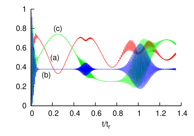
Figure 4: (color online) Time evolution for a system with two qubits when $\bar{n}=50$ for two different initial states of the qubits. (Top)The initial state of the qubits is ${\left|gg\right\rangle}$ and it can be seen that the two qubit ‘attractor’ state is not reached at ${\textstyle\frac{t_{r}}{4}}$. (Bottom) The initial state of the qubits is $\frac{1}{\sqrt{2}}({\left|ee\right\rangle}+{\left|gg\right\rangle})$ (i.e. within the basin of attraction) and it shows that the two qubit ‘attractor’ state is reached at ${\textstyle\frac{t_{r}}{4}}$.
In both diagrams (a) the entropy of the qubits. (b) the probability of the two qubit state ${\left|gg\right\rangle}$. (c) the probability of being in the two qubit ‘attractor’ state ${\left|\psi_{2\,att}^{+}\right\rangle}$ when the initial phase of the radiation field is $\theta=0$.

A second dip in the entropy can be seen in Fig. 4 at the time $t=\frac{3t_{r}}{4}$ which, in the large $\bar{n}$ approximation, goes to zero. The probability of being in the ‘attractor’ state ${\left|\psi^{+}_{2\,att}\right\rangle}$ goes to zero at this time. The field has disentangled itself from the field again, so at this point the qubits are again in a pure state, the orthogonal ‘attractor’ state ${\left|\psi_{1\,att}^{-}\right\rangle}$.

It can be seen from the analytic solution that, in the large $\bar{n}$ approximation, the field and qubits also disentangle themselves at the time $t_{r}$, for all initial conditions of the qubits, and also at ${\textstyle\frac{t_{r}}{2}}$ if the initial qubit state is in the basin of attraction. This is not seen in the diagrams in Fig. 4 and instead the value to the entropies at these times are fairly high which means the numerically evaluated exact system is far from the analytic results in large $\bar{n}$ approximation. This is similar to the one qubit case and can be explained by considering the dynamics of the field.

We can once again plot the $Q$ function for the numerical solution to pictorially display what is occurring in the cavity field. The values of $Q(\alpha,t)$ in the complex $\alpha$ plane at fixed times are shown in Fig. 5 when the qubits are initially in the state ${\left|gg\right\rangle}$, which is outside the basin of attraction. This time the $Q$ function shows a set of three wavepackets of the cavity field (compared to the two for the one-qubit case, Fig. 2). As a function of time the three ‘blobs’ separate, but only two move around the complex plane and follow the circular path of radius $\sqrt{\bar{n}}$. Again the arrows show the dipole moment of the qubit state associated with each wavepacket, $\overrightarrow{d_{k}}(t)={\left\langle D_{k}(t)\right|}\overrightarrow{\hat{J_{2}}}{\left|D_{k}(t)\right\rangle}$. The ‘blob’ that does not move over time has a dipole moment of zero, so only the two moving Gea-Banacloche states have an arrow.

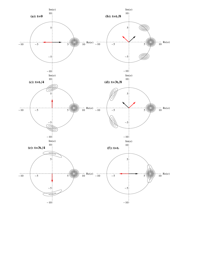
Figure 5: (color online) The $Q$ function at six different times when the qubits are initially in the state ${\left|gg\right\rangle}$. Once again the atomic dipole states are represented as arrows and $\bar{n}=50$. (a) the time $t=0$. The system is started in a coherent state which is shown by a circle of uncertainty in phase space. (b) a time a little after that of figure (a), $t={\textstyle\frac{t_{r}}{8}}$. (c) the time $t={\textstyle\frac{t_{r}}{4}}$. (d) the time $t=\frac{3t_{r}}{8}$. (e) the time $\frac{3t_{r}}{4}$. (f) the time $t=t_{r}$. Both the wavepackets have returned to their original position.

For the one-qubit case the revival time occurred when the two wavepackets overlapped. In this case we have two ‘blobs’ that move around phase space and overlap at the time $t={\textstyle\frac{t_{r}}{2}}$, leaving the stationary wavepacket at the initial position. This causes a rather weak revival peak as only two of the three wavepackets are in phase. At a later time, Fig. 5(f), all three wavepackets converge at the starting position and there is a main revival peak, $t=t_{r}$. If the initial state of the qubits was in the basin of attraction then $\beta_{0}\approx 0$ and there would only be two wavepackets. The $Q$ function pictures would then look similar to those in Fig. 2 and the system would behave like the one-qubit case. Nevertheless we note that the radiation field returns to the start position after one revival time, $t_{r}$ compared to the one-qubit case where it returns to the same place after $2t_{r}$.

In summary when there are two qubits interacting with a single cavity mode the wavefunction consists of a part that behaves like the one qubit case, ${\left|D_{\pm 1}(t)\right\rangle}$ and an extra part ${\left|D_{0}\right\rangle}$. The ‘attractor’ state, ${\left|\psi_{2\,att}^{\pm}\right\rangle}$, occurs at the times when the two ‘blobs’ in phase space are macroscopically different and when $\beta_{0}=0$. Moving from the one qubit case to the two qubit case involves a mapping of $t\rightarrow 2t$ and a similar mapping can be used to understand the equations for more qubits.

III.2 Collapse and Revival of Entanglement

An interesting new feature of the two-qubit case, as opposed to the one-qubit case, is that there can be entanglement present between the two qubits themselves, not just between the qubits and the field. So far we have used the entropy to measure the amount of entanglement between the field and the qubit system as the whole system is in a pure state. Unfortunately this measure can not be used to calculate the entanglement between the two qubits as they are sometimes in a mixed state themselves. To find the amount of entanglement between the two qubits we use the mixed state tangle $\tau$, defined as W. K. Wootters (1998, 2001):

$$\tau=[\mathrm{max}\{\lambda_{1}-\lambda_{2}-\lambda_{3}-\lambda_{4},0\}]^{2}.$$ (35)

The $\lambda^{\prime}s$ are the square root of the eigenvalues, in decreasing order, of the matrix $\rho_{q}\left(\sigma^{y}\otimes\sigma^{y}\right)\rho_{q}^{\ast}\left(\sigma^{y}\otimes\sigma^{y}\right)$, where $\sigma^{y}=i\left(\sigma^{-}-\sigma^{+}\right)$ (see equation Eq. 3) and $\rho_{q}^{\ast}$ represents the complex conjugate of $\rho_{q}$ in the ${\left|e\right\rangle}$, ${\left|g\right\rangle}$ basis. A tangle of unity indicates that there is maximum entanglement between the two qubits. If the tangle takes the value of zero, then there is no entanglement present between the two qubits. To clarify, the entropy will be used to measure the amount of entanglement between the field and the qubit system whereas the tangle will be used to measure the entanglement between the qubits.

In this subsection we focus on the initial states inside the basin of attraction. The value of the tangle for the states given by Eq. (33) can be seen in Fig. 6. This diagram shows only two points where $\tau=0$, for $a=\pm\frac{1}{2}$, which demonstrates that there are only two product states in the ‘basin of attraction’. In contrast, there are many points in which $\tau=1$, for $a=\frac{e^{i\phi}}{\sqrt{2}}$ where $\phi$ is an arbitrary phase, or $a=ir$ where $r$ is a real number. This means that all possible levels of entanglement are represented in the basin of attraction, Eq. (33).

Figure 6: (color online) The value of the tangle for the states in the basin of attraction, for different values of $a$. We notice that the plot shows only two points where the tangle is zero.

Whilst almost all states in the basin of attraction given in Eq. (33) describe entangled states, these all evolve into ${\left|\psi_{2\,att}^{+}\right\rangle}$ at $t={\textstyle\frac{t_{r}}{4}}$ and ${\left|\psi_{2\,att}^{-}\right\rangle}$ at $t=\frac{3t_{r}}{4}$, at which times they are pure and unentangled. So if the system is started off in one of these entangled states defined by Eq. (33), at the time ${\textstyle\frac{t_{r}}{4}}$ the system goes to a state which has zero entanglement. Therefore we have gone from having entanglement in the system to having absolutely no entanglement, either between the qubits and the resonator or between the qubits themselves. At a later time this entanglement returns to the system and can be said to ‘revive’. The tangle returns to its initial value at ${\textstyle\frac{t_{r}}{2}}$ and $t_{r}$, regardless of the phase of the coherent state. This can be seen when we consider the wavefunction for the system at this time:

$${\left|\widetilde{\Psi}_{2}({\textstyle\frac{t_{r}}{2}})\right\rangle} = -\frac{1}{2}{\left|-\alpha\right\rangle}\left[e^{i\pi\bar{n}}\left(a-\sqrt{\frac{1}{2}-{\left|a\right|}^{2}}\right)\left(e^{-i\theta}{\left|ee\right\rangle}+{\left|eg\right\rangle}+{\left|ge\right\rangle}+e^{i\theta}{\left|gg\right\rangle}\right)\right.$$ (36)

$$+ \left.e^{-i\pi\bar{n}}\left(a+\sqrt{\frac{1}{2}-{\left|a\right|}^{2}}\right)\left(e^{-i\theta}{\left|ee\right\rangle}-{\left|eg\right\rangle}-{\left|ge\right\rangle}+e^{i\theta}{\left|gg\right\rangle}\right)\right].$$

As stated in Sec. III.1 this state shows no entanglement between the qubits and the field and therefore the entropy of the reduced qubit density matrix will be zero. The value of the tangle for the qubit state at $t={\textstyle\frac{t_{r}}{2}}$ is found to be exactly the same as the tangle for the initial state of the qubits, therefore $\tau(0)=\tau({\textstyle\frac{t_{r}}{2}})$. We have called this phenomenon ‘Collapse and Revival of Entanglement’ C. E. A. Jarvis, D. A. Rodrigues, B. L. Györffy, T. P. Spiller, A. J. Short and J. F. Annett (2008). Analogous to the single qubit case, the quantum information in the initial state of the qubits (for states within the basin of attraction) is swapped out and encoded into the field state at the ‘attractor’ times. Calculations demonstrate that the value of the tangle remains near zero for long periods between revival. Therefore we are dealing with a phenomenon which has been described as the ‘death of entanglement’ by Yu and Eberley Ting Yu and J. H. Eberly (2004, 2009) which forms the centre of much current interest J. H. Eberly and Ting Yu (2007). Qing et al. Yang Qing, Yang Ming and Cao Zhuo-Liang (2008) have found a similar collapse and revival for the same model we have studied here but for very different initial conditions. Even just within the system we consider here, detailed studies reveal interesting links between the dynamics of the disappearance (and reappearance) of entanglement and the basin of attraction, as we discuss in this and the subsequent subsection.

So if the qubit system starts in the basin of attraction and $\tau\neq 0$, over time the initial entanglement in the qubits is exchanged for entanglement between the qubits and the field, and then for a superposition of field states. At the time of the ‘attractor’ state, ${\textstyle\frac{t_{r}}{4}}$, there is absolutely no entanglement present in the system. Then the process starts to reverse. Firstly there is again entanglement between the qubits and the field and at the two qubit revival time, ${\textstyle\frac{t_{r}}{2}}$, $\tau$ returns to its initial value and only qubit entanglement is present.

The actual extent of the entanglement revival for the exact solution can be seen in Fig. 7 (a) where we show the tangle for different initial states within the basin of attraction. On first glance we see that the amount of tangle present at $t={\textstyle\frac{t_{r}}{2}}$ is nowhere near the initial amount of tangle present at $t=0$, which is far from the prediction in the large $\bar{n}$ approximation. The value of the entropy at ${\textstyle\frac{t_{r}}{2}}$ is around $0.5$ for the case when $a={\textstyle\frac{1}{\sqrt{2}}}$, rather than the predicted value of zero, Fig. 7 (b). In order for there to be maximum possible entanglement in the system there has to be the least amount of entropy, so there is a trade off in tangle for entropy W. J. Munro, D. F. V. James, A. G. White, and P. G. Kwiat (2001).

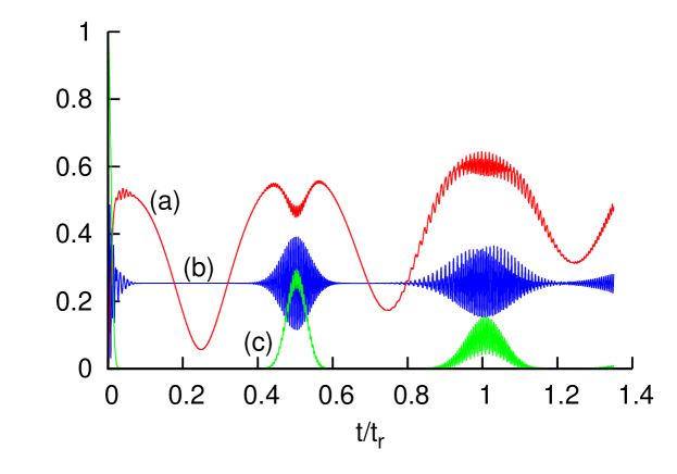
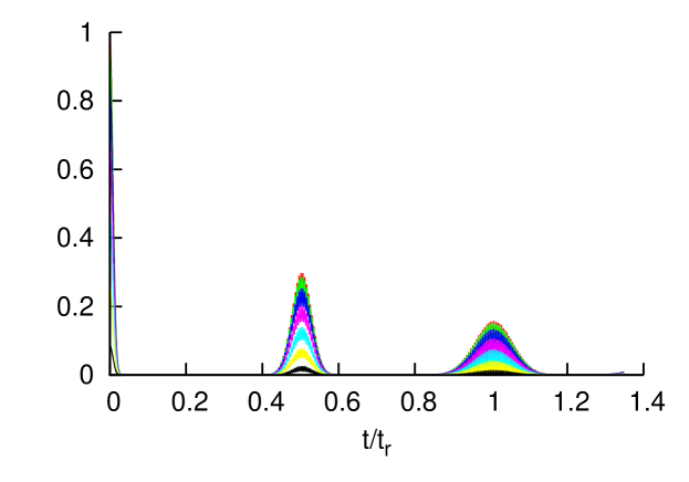
Figure 7: (color online) (Top) ‘Collapse and Revival of Entanglement’ when the qubits are started in the maximally entangled state $({\left|ee\right\rangle}+{\left|gg\right\rangle})/\sqrt{2}$ where $\bar{n}=50$. (a) the entropy of the qubits. (b) the probability of the two qubit state ${\left|gg\right\rangle}$. (c) the tangle for the system.
(Bottom)‘Collapse and Revival of Entanglement’ for many different initial qubit states in the basin of attraction with $\bar{n}=50$. These are shown in many different colours depending on the initial entanglement measure. It shows that the entanglement in the qubits is initially lost then returns at the first revival peak, $t={\textstyle\frac{t_{r}}{2}}$. As the initial state is in the basin of attraction we know the whole system has zero entanglement at $t={\textstyle\frac{t_{r}}{4}}$. So there is even no entanglement between the field and the qubits. Therefore we know that over time the amount of entanglement varies a great deal.

Another very interesting feature illustrated in Fig. 7 (a) is the manner in which the entanglement vanishes. For all states within the basin of attraction, although the initial entanglement decays rapidly (before reviving at ${\textstyle\frac{t_{r}}{2}}$ and later times) it does so with a Gaussian envelope (as per the Rabi oscillation collapse). It therefore goes smoothly to zero—this is reflected by the further observation that the eigenvalue expression in Eq. (35) never goes negative, so the max operation never needs to be implemented for the tangle. This can be explained by considering the rank of the matrix used to calculate the tangle, $\rho_{q}\left(\sigma^{y}\otimes\sigma^{y}\right)\rho_{q}^{\ast}\left(\sigma^{y}\otimes\sigma^{y}\right)$. The rank of a matrix is equal to the number of non-zero eigenvalues. The matrix used to calculate the tangle for this system has a maximum of rank$=2$ when the qubits are started in the basin of attraction, so $\lambda_{3}=\lambda_{4}=0$. Due to the definition of the tangle, $\lambda_{1}\geq\lambda_{2}$ and Eq. (35) becomes:

$$\tau=(\lambda_{1}-\lambda_{2})^{2}\geq 0.$$ (37)

This characteristic ‘Collapse and Revival’ behaviour is to be contrasted with behaviour where entanglement vanishes or appears with finite gradient and where the $\mathrm{max}$ operation is needed in Eq. (35) because the eigenvalue expression does go negative. To distinguish these behaviours, we use the terminology ‘sudden death/birth’ of entanglement Ting Yu and J. H. Eberly (2004) for the latter. This phenomenon does not occur for initial qubit states within the basin of attraction (which all show collapse and revival of entanglement) but can for those outside, as will be demonstrated in the next subsection.

III.3 Outside the Basin of Attraction

The previous subsections discussed interesting features of the entanglement dynamics for the two-qubit JCM when considering initial conditions inside the basin of attraction. In this subsection we highlight interesting features that emerge when considering all other cases—when the qubit Hilbert space is not restricted and, for example, the terms $(b{\left|eg\right\rangle}+\sqrt{1-{\left|b\right|}^{2}}{\left|ge\right\rangle})/\sqrt{2}$, where $b$ is a complex number, are present in the initial state, as well as unequal superpositions of ${\left|gg\right\rangle}$ and ${\left|ee\right\rangle}$. To date, in other works it has been found that the JCM for two qubits can exhibit an interesting phenomenon called ‘Sudden Death of Entanglement’, for certain initial conditions of the qubits. Some investigations start with the qubits and the field in a mixed state and some others do not Yang Qing, Yang Ming and Cao Zhuo-Liang (2008).

In our work we consider the case when the radiation field is started in a coherent state. Qubits states inside the basin of attraction demonstrate collapse and revival of entanglement, but not sudden death or birth. However, if we venture outside the basin of attraction and include other initial conditions of the two qubit system, we find that there is indeed sudden death of entanglement. This means that we do not restrict the condition $\beta_{0}=0$ in Eq. (23).

Now, without this restriction, the qubit system will not go towards the ‘attractor’ state at ${\textstyle\frac{t_{r}}{4}}$ and $\frac{3t_{r}}{4}$ in the large $\bar{n}$ approximation as $\beta_{0}\neq 0$. Furthermore the entropy will be non zero at these times as the qubit state can not be factorised out of the wavefunction. However, the system will still have zero entropy at the ‘full’ revival time $t_{r}$ as ${\left|\Phi_{-1}(t_{r})\right\rangle}={\left|\Phi_{0}(t_{r})\right\rangle}={\left|\Phi_{+1}(t_{r})\right\rangle}={\left|\alpha\right\rangle}$ and the field state can be factorised out of the wavefunction. Like before $\tau(0)=\tau(t_{r})$ so the amount of entanglement between the qubits is the same at the main revival time and $t=0$. For $\bar{n}=50$, this revival will not be complete and so the tangle will not return to its initial value. Fig. 8 shows examples of the qubit entanglement dynamics for initial states which are outside the basin of attraction for the numerically evaluated exact solution. In this figure a new measure of qubit entanglement has been used called the concurrence $\zeta=\sqrt{\tau}$ and has been used as a direct comparison to previous work J. H. Eberly and Ting Yu (2007); Ting Yu and J. H. Eberly (2009); Muhammed Yönaç, Ting Yu and J H Eberly (2006).

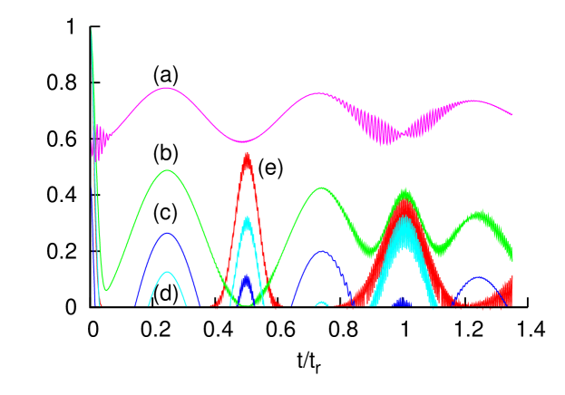
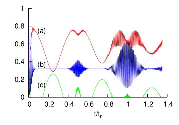
Figure 8: (color online) (Top) Values of the concurrence over time for several different initial qubit states. As in previous figures, $\bar{n}=50$. (a) The initial state of the qubits is $\frac{1}{\sqrt{10}}{\left|ee\right\rangle}-\sqrt{\frac{9}{10}}{\left|gg\right\rangle}$. At times the concurrence is greater than the initial value. (b) The initial state of the qubits is $\frac{1}{\sqrt{2}}\left({\left|eg\right\rangle}+i{\left|ge\right\rangle}\right)$, and unlike initial conditions within the basin of attraction, leads to a concurrence value of zero at ${\textstyle\frac{t_{r}}{2}}$. (c) The initial state of the qubits is $\frac{1}{\sqrt{20}}{\left|ee\right\rangle}+\sqrt{\frac{19}{20}}{\left|gg\right\rangle}$ and shows ‘Sudden Death of Entanglement’. (d) The initial state of the qubits is $\frac{1}{\sqrt{2}}\left({\left|eg\right\rangle}+e^{\frac{i\pi}{4}}{\left|ge\right\rangle}\right)$, a maximally entangled state that exhibits ‘Sudden Death of Entanglement’. (e) The initial state of the qubits is $\frac{1}{\sqrt{2}}\left({\left|ee\right\rangle}+{\left|gg\right\rangle}\right)$, a maximally entangled state that lies in the basin of attraction that is used as a comparison.
(Bottom) ‘Sudden Death of Entanglement’ when the qubits are started in the state $\frac{1}{\sqrt{20}}{\left|ee\right\rangle}+\sqrt{\frac{19}{20}}{\left|gg\right\rangle}$, case (c) in the top diagram. As before (a) the entropy of the qubits. (b) the probability of the qubit being in the state ${\left|gg\right\rangle}$. (c) the mixed state concurrence of the qubit system.

Remarkably, Fig. 8 shows that a field initially in a coherent state can give sudden death and birth of entanglement, with initial qubit states of various forms lying outside the basin of attraction. A case where the initial conditions are in the basin of attraction is shown for reference. Clearly peaks in the entanglement measure at both ${\textstyle\frac{t_{r}}{4}}$ and $\frac{3t_{r}}{4}$ arise (with death/birth at finite gradient)—times when there would be no entanglement if the initial qubit state was in the basin of attraction. There are still peaks at the times ${\textstyle\frac{t_{r}}{2}}$ and $t_{r}$, but these have a lower maximum and also now exhibit birth/death behaviour rather than Gaussian collapse and revival. One initial condition that yields ‘Sudden Death of Entanglement’ has been shown in Fig. 8 alongside an entropy measurement.

To recap, we find that our system can display both a sudden birth/death of entanglement as well as a Gaussian collapse and revival of entanglement, depending on initial conditions. Furthermore, we understand that, in this system, the sudden death occurs when $\lambda_{1}-\lambda_{2}-\lambda_{3}-\lambda_{4}$ becomes negative and so, according due to the max operation used in Eq. 35 the tangle goes to zero with a finite gradient. In contrast, within the basin of attraction, there are only two non-zero eigenvalues $\lambda_{1}>\lambda_{2}$, so the tangle can only display a smooth collapse.

These additional peaks in the qubit entanglement seen in Fig. 8 are due to the inclusion of ${\left|D_{0}\right\rangle}$ and ${\left|\Phi_{0}(t)\right\rangle}$ in the wavefunction. From the analysis in Sec. III we showed that ${\left|D_{\pm 1}({\textstyle\frac{t_{r}}{4}})\right\rangle}={\left|\psi_{2\,att}^{+}\right\rangle}$, the unentangled two qubit ‘attractor’ state, so all entanglement present at $t={\textstyle\frac{t_{r}}{4}}$ is due to ${\left|D_{0}\right\rangle}$. If ${\left|D_{0}\right\rangle}$ is a product state then there will be no entanglement in the qubit system. However if ${\left|D_{0}\right\rangle}$ is entangled it still does not mean there will be some qubit entanglement as a mixture of entangled and product states need not be entangled. For example curve (b) in the top diagram of Fig. 8 shows there is zero concurrence at $\frac{t_{r}}{2}$, even though ${\left|D_{0}\right\rangle}$ contains some entanglement.

IV $N_{q}$ qubit Jaynes-Cummings Model

Having found a sense in which the one qubit ‘attractor’ state has analogues for two qubits, it is natural to inquire whether similar generalisation holds for the case of more than two qubits. We use the Hamiltonian shown in Eq. (19) for $N_{q}$ qubits. We have found that there are indeed cases where the system goes to a state similar to the one qubit ‘attractor’ state and have a general form for the basin of attraction for $N_{q}$ qubits.

In the large $\bar{n}$ approximation the state of the system takes the following form T. Meunier, A. Le Diffon, C. Ruef, P. Degiovanni and J.-M. Raimond (2006):

$${\left|\widetilde{\Psi}_{N_{q}}(t)\right\rangle}=\sum_{k=-N_{q}/2}^{N_{q}/2}\beta_{k}(t){\left|D_{k}(t)\right\rangle}\otimes{\left|\Phi_{k}(t)\right\rangle}.$$ (38)

${\left|D_{k}(t)\right\rangle}$ has a complicated form and occurs in the paper by Meunier et al. T. Meunier, A. Le Diffon, C. Ruef, P. Degiovanni and J.-M. Raimond (2006). For this work we will be most concerned with the states that appear in the expression for the basin of attraction. These take the following simple form:

$${\left|D_{\pm\frac{N_{q}}{2}}(t)\right\rangle} = {\left|D_{\pm\frac{1}{2}}(N_{q}\,t)\right\rangle}\otimes\ldots\otimes{\left|D_{\pm\frac{1}{2}}(N_{q}\,t)\right\rangle}$$ (39)

$$= {\left|D_{\pm\frac{1}{2}}(N_{q}\,t)\right\rangle}^{\otimes N_{q}}.$$ (40)

Note that:

$${\left|\Phi_{k}(t)\right\rangle}={\left|e^{i\pi kN_{q}t/t_{r}}\alpha\right\rangle},$$ (41)

and we can use this equation to understand the simple dynamics of the $N_{q}$ solution. The field initially starts in a coherent state that then splits into $N_{q}+1$ different ‘blobs’ and a revival peak occurs every time at least two of these wavepackets overlaps. The strength of the revival is determined by the number of wavepackets that overlap and these revival peaks occur at definite intervals. Using Eq. (41) we can write a general form for the revival times:

$$\left(k+\frac{1}{p}\right)t_{r},\ \ \ \left(k+\frac{(p-1)}{p}\right)t_{r},\ \ \ p=1,2,...,N_{q}\ \ {\rm{and}}\ \ k=1,2,...,\infty.$$ (42)

Eq. (41) also highlights that when there are an even number of qubits the field returns to its initial state ${\left|\alpha\right\rangle}$ after a time of $t_{r}$. The time till the wavepackets return to their original position is determined by the slowest moving wavepackets, which are ${\left|e^{\pm 2i\pi t/t_{r}}\alpha\right\rangle}$ in the even qubit case and ${\left|e^{\pm i\pi t/t_{r}}\alpha\right\rangle}$ in the odd qubit case. When $N_{q}$ is odd the wavepackets return to their start position after a time $2t_{r}$ and there will always be no stationary wavepacket at the start position.

A sketch of the $Q$ function of the field for three qubits is shown in Fig. 9 for large values of $\bar{n}$ and we once again show the dipole moments as arrows. Using ${\left|D_{k}\right\rangle}$ in reference T. Meunier, A. Le Diffon, C. Ruef, P. Degiovanni and J.-M. Raimond (2006) we can compute a general term for the equation of the dipole moments in the large $\bar{n}$ approximation and is shown below.

$$\overrightarrow{d}_{k} = {\left\langle D_{k}\right|}\overrightarrow{\hat{J}}_{N_{q}}{\left|D_{k}\right\rangle}={\left\langle D_{k}\right|}\overrightarrow{\hat{\sigma}}_{N_{q}}{\left|D_{k}\right\rangle}$$ (43)

$$= {\left|k\right|}\left(\pm\cos\left(\theta+\frac{2{\left|k\right|}\pi t}{t_{r}}\right)\underline{\hat{i}}+\sin\left(\theta+\frac{2{\left|k\right|}\pi t}{t_{r}}\right)\underline{\hat{j}}\right)$$

where $\overrightarrow{\hat{\sigma}}_{N_{q}}=\hat{\sigma}_{N_{q}}^{x}\underline{\hat{i}}+\hat{\sigma}_{N_{q}}^{y}\underline{\hat{j}}+\hat{\sigma}_{N_{q}}^{z}\underline{\hat{k}}$, is the Pauli vector for $N_{q}$ qubits and

$$\hat{\sigma}_{N_{q}}^{x,y,z} = \sum^{N_{q}}_{i=1}\hat{\sigma}^{x,y,z}_{i}.$$ (44)

Figure 9: (color online) Phase space sketches of the $Q$ function at eight different times when the qubits are initial started in the state ${\left|ggg\right\rangle}$. The atomic dipole states are represented as arrows. (a) the time $t=0$. The system is started in a coherent state which is shown by a circle of uncertainty in phase space. (b) a time a little after $t=0$. (c) the time $t={\textstyle\frac{t_{r}}{6}}$. (d) the time $t={\textstyle\frac{t_{r}}{3}}$. (e) the time $t={\textstyle\frac{t_{r}}{2}}$. (f) the time $t={\textstyle\frac{2t_{r}}{3}}$. (g) the time $t={\textstyle\frac{5t_{r}}{6}}$. (h) the time $t=t_{r}$.

We notice again the pattern of the arrows changes over time and that the wavepackets come to their original starting position after a time $2t_{r}$.

IV.1 Basin of Attraction

Using the above experience with one and two qubits, we investigate whether a basin of attraction exists for $N_{q}>2$. Using the expansion pioneered by Chumakov et al. S. M. Chumakov, A. B. Klimov and J. J. Sanchez-Mondragon (1994) and developed independently by Meunier et al. T. Meunier, A. Le Diffon, C. Ruef, P. Degiovanni and J.-M. Raimond (2006) we have indeed found a basin of attraction for $N_{q}$ qubits. As ${\left|D_{\pm\frac{1}{2}}({\textstyle\frac{t_{r}}{2}})\right\rangle}={\left|\psi_{1\,att}^{+}\right\rangle}$, and using the observation made in Eq. (40), we can therefore conclude that ${\left|D_{\pm\frac{N_{q}}{2}}(t)\right\rangle}$ will go to a direct product of ${\left|\psi_{1\,att}^{+}\right\rangle}$ at $t={\textstyle\frac{t_{r}}{2N_{q}}}$.

$${\left|D_{\pm\frac{N_{q}}{2}}\left({\textstyle\frac{t_{r}}{2N_{q}}}\right)\right\rangle} = {\left|D_{\pm\frac{1}{2}}({\textstyle\frac{t_{r}}{2}})\right\rangle}^{\otimes N_{q}}$$ (45)

$$= {\left|\psi^{+}_{1\,att}\right\rangle}^{\otimes N_{q}}$$ (46)

$$= {\left|\psi^{+}_{N_{q}\,att}\right\rangle}$$ (47)

By setting the values of $\beta_{p}(t)=0$, for $p={\textstyle\frac{N_{q}-2}{2}},...,-{\textstyle\frac{N_{q}-2}{2}}$ then only ${\left|D_{\pm\frac{N_{q}}{2}}(t)\right\rangle}$ are in the wavefunction and the qubits will go to ${\left|\psi_{N_{q}\,att}^{+}\right\rangle}$ at $t={\textstyle\frac{t_{r}}{2N_{q}}}$. Using this information we have found a basin of attraction for $N_{q}$ qubits.

$${\left|\psi_{N_{q}}\right\rangle} = \sum_{m=-N_{q}/2}^{N_{q}/2}\frac{A(N_{q},a,m)e^{-i(\frac{N_{q}}{2}-m)\theta}\sqrt{N_{q}!}}{\sqrt{\left(\frac{N_{q}}{2}+m\right)!\left(\frac{N_{q}}{2}-m\right)!}}{\left|N_{q},m\right\rangle}$$

$$A(N_{q},a,m) = \left\{\begin{array}[]{cc}a&\text{if $\left(\frac{N_{q}}{2}-m\right)$ is even}\\ &\\ \sqrt{\frac{1}{2^{N_{q}-1}}-{\left|a\right|}^{2}}&\text{if $\left(\frac{N_{q}}{2}-m\right)$ is odd}\end{array}\right.$$ (51)

As before $\phi$ is an arbitrary phase and $\theta$ is the initial phase of the radiation field with $0\leq{\left|a\right|}\leq\frac{1}{\sqrt{2^{N_{q}-1}}}$. The basin of attraction is in the symmetric subspace and ${\left|N_{q},m\right\rangle}$ is the symmetrised state with $N_{e}$ excited qubits, $N_{g}$ qubits in the ground state and $m=\frac{N_{e}-N_{g}}{2}$. For example, for the three qubit case, ${\left|N_{q}=3,m=\frac{1}{2}\right\rangle}={\textstyle\frac{1}{\sqrt{3}}}\left({\left|eeg\right\rangle}+{\left|ege\right\rangle}+{\left|gee\right\rangle}\right)$ as $N_{e}=2$ and $N_{g}=1$ etc. We note that although the state space of the qubits increases with increasing $N_{q}$, the basin of attraction is still parameterised by the single complex value $a$. The significance of this will become apparent in Sec. IV.2.

We emphasise that when the qubits start in the basin of attraction then there are only two wavepackets in phase space of the photon field for all time. The initial conditions have restricted the system to behave like the one qubit case as is highlighted by considering the wavefunction at $t={\textstyle\frac{t_{r}}{2N_{q}}}$.

$${\left|\widetilde{\Psi}_{N_{q}}\left({\textstyle\frac{t_{r}}{2N_{q}}}\right)\right\rangle}={\left|\psi^{+}_{N_{q}\,att}\right\rangle}\left(\beta_{{\textstyle\frac{N_{q}}{2}}}\left({\textstyle\frac{t_{r}}{2N_{q}}}\right){\left|i\alpha\right\rangle}+\beta_{-{\textstyle\frac{N_{q}}{2}}}\left({\textstyle\frac{t_{r}}{2N_{q}}}\right){\left|-i\alpha\right\rangle}\right)$$ (52)

In the one qubit case the qubit system also goes to a second ‘attractor’ state ${\left|\psi_{1\,att}^{-}\right\rangle}$ at the time ${\textstyle\frac{3t_{r}}{2}}$ and so ${\left|D_{\pm\frac{N_{q}}{2}}\left(\frac{3t_{r}}{2N_{q}}\right)\right\rangle}={\left|\psi^{-}_{1\,att}\right\rangle}^{\otimes N_{q}}={\left|\psi^{-}_{N_{q}\,att}\right\rangle}$. Qubits started in the basin of attraction, Eq. (IV.1), will go to these ‘attractor’ states and hence the entropy will go to zero.

We can construct a series for when these ‘attractor’ times will occur for $N_{q}$ qubits, shown in table 1 with the revival times from Eq. (42). The general equation for these times is:

$$\left(k+\frac{(2p-1)}{2N_{q}}\right)t_{r},\ \ \ \ \ \ p=1,2,...,N_{q}\ \ {\rm{and}}\ \ k=1,2,...,\infty.$$ (53)

No. of qubits	No. of Blobs	Revival Times	Possible ‘Attractor’ Times
1	2	$t_{r}$	$\frac{t_{r}}{2}$
2	3	$\frac{t_{r}}{2}$, $t_{r}$	$\frac{t_{r}}{4}$, $\frac{3t_{r}}{4}$
3	4	$\frac{t_{r}}{3}$, $\frac{t_{r}}{2}$, $\frac{2t_{r}}{3}$, $t_{r}$	$\frac{t_{r}}{6}$, $\frac{t_{r}}{2}$, $\frac{5t_{r}}{6}$
4	5	$\frac{t_{r}}{4}$, $\frac{t_{r}}{3}$, $\frac{t_{r}}{2}$, $\frac{2t_{r}}{3}$, $\frac{3t_{r}}{4}$, $t_{r}$	$\frac{t_{r}}{8}$, $\frac{3_{r}}{8}$, $\frac{5t_{r}}{8}$, $\frac{7t_{r}}{8}$
5	6	$\frac{t_{r}}{5}$, $\frac{t_{r}}{4}$, $\frac{t_{r}}{3}$, $\frac{t_{r}}{2}$, $\frac{2t_{r}}{3}$, $\frac{3t_{r}}{4}$, $\frac{4t_{r}}{5}$, $t_{r}$	$\frac{t_{r}}{10}$, $\frac{3t_{r}}{10}$, $\frac{t_{r}}{2}$, $\frac{7t_{r}}{10}$, $\frac{9t_{r}}{10}$

Table 1: A summary of where the different revival peaks occur for differing numbers of qubits. Also the times are shown for when ${\left|D_{\pm\frac{N_{q}}{2}}\left(t\right)\right\rangle}={\left|\psi^{\pm}_{N_{q}\,att}\right\rangle}$. Note that only revival and ‘attractor’ times in the interval $0<t\leq t_{r}$ are shown. Further times can be obtained by adding integer multiples of $t_{r}$.

In Fig. 10 we show the $3$ and $4$ qubit evolution starting in a state in the basin of attraction (Eq. (IV.1)). In general we do see there are dips in the entropy that go close to zero and the probability of being in the ‘attractor’ state goes to close to one. These features get more pronounced as $\bar{n}$ is increased. As for the two-qubit case, when this probability goes to zero, the system is in the second ‘attractor’ state, ${\left|\psi^{-}_{N_{q}\,att}\right\rangle}$, which is orthogonal to the first.

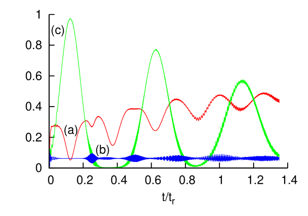
Figure 10: (color online) Time evolution of the system when the initial qubit state is in the basin of attraction for $\bar{n}=50$ and $\theta=0$. (Top) Three qubits: The initial state of the qubits is $\frac{1}{2}\left({\left|N_{q}=3,m={\textstyle\frac{3}{2}}\right\rangle}+\sqrt{3}{\left|N_{q}=3,m=-\frac{1}{2}\right\rangle}\right)$. (Bottom) Four qubits: The initial state of the qubits is $\frac{1}{\sqrt{2}}({\left|N_{q}=4,m=1\right\rangle}+{\left|N_{q}=4,m=-1\right\rangle})$. As before (a) the entropy of the qubits. (b) the probability of all the qubits being in the state ${\left|g\right\rangle}$. (c) the probability of being in the qubit ‘attractor’ state ${\left|\psi_{N_{q}\,att}^{+}\right\rangle}$.

IV.2 Collapse and Revival of ‘Schrödinger Cat’ States

Surprisingly, the basin of attraction has a simple form when written in terms of spin coherent states, which are analogous to coherent states of a photon field. As described in Appendix A, such states are given by:

$${\left|z,N_{q}\right\rangle} = \frac{1}{(1+{\left|z\right|}^{2})^{N_{q}/2}}\sum_{m=-N_{q}/2}^{N_{q}/2}\sqrt{\frac{N_{q}!}{(\frac{N_{q}}{2}-m)!(\frac{N_{q}}{2}+m)!}}z^{(\frac{N_{q}}{2}-m)}{\left|N_{q},m\right\rangle}$$ (54)

$$= \frac{1}{(1+{\left|z\right|}^{2})^{N_{q}/2}}\left({\left|e\right\rangle}+z{\left|g\right\rangle}\right)^{\otimes N_{q}}$$ (55)

where ${\left|N_{q},m\right\rangle}$ is defined in Sec. IV.1. A spin coherent state is a product state and this is easily seen when it is written in Majorana representation E. Majorana (1932) in Eq. (55). Below we rewrite Eq. (IV.1) in the form of a superposition of two spin coherent states, and show the form of the wavefunction at the time $t=0$ when the qubits are in the basin of attraction:

$${\left|\widetilde{\Psi}_{N_{q}}(0)\right\rangle}={\left|\psi_{N_{q}}\right\rangle}{\left|\alpha\right\rangle} = \left(\sqrt{2^{N_{q}-2}}\left(a+\sqrt{\frac{1}{2^{N_{q}-1}}-{{\left|a\right|}}^{2}}\right){\left|z=e^{-i\theta},N_{q}\right\rangle}\right.$$ (56)

$$+ \left.\sqrt{2^{N_{q}-2}}\left(a-\sqrt{\frac{1}{2^{N_{q}-1}}-{{\left|a\right|}}^{2}}\right){\left|z=-e^{-i\theta},N_{q}\right\rangle}\right){\left|\alpha\right\rangle}$$

From Eq. (55) it is clear that ${\left|z=e^{-i\theta},N_{q}\right\rangle}$ is orthogonal to ${\left|z=-e^{-i\theta},N_{q}\right\rangle}$ and ${\left|\psi_{N_{q}}\right\rangle}$ is a collection of spin ‘Schrödinger cat’ states. We also write the state of the field at the time of the first dip in the entropy for an arbitrary number of qubits, $t={\textstyle\frac{t_{r}}{2N_{q}}}$:

$${\left|\widetilde{\Psi}_{N_{q}}({\textstyle\frac{t_{r}}{2N_{q}}})\right\rangle} = {\left|\psi_{N_{q}\,att}^{+}\right\rangle}\left(\sqrt{2^{N_{q}-2}}\left(a-\sqrt{\frac{1}{2^{N_{q}-1}}-{{\left|a\right|}}^{2}}\right)e^{i\pi\bar{n}/2}{\left|i\alpha\right\rangle}\right.$$ (57)

$$-\left.\sqrt{2^{N_{q}-2}}\left(a+\sqrt{\frac{1}{2^{N_{q}-1}}-{{\left|a\right|}}^{2}}\right)e^{-i\pi\bar{n}/2}{\left|-i\alpha\right\rangle}\right)$$

Eq. (56) and Eq. (57) are very similar and show how a Schrödinger cat state, and the information about the initial conditions of the qubits, moves from the qubits to the field. At the time $t=0$ the qubits are in a spin ‘Schrödinger cat’ state and the variable $a$, which fixes the initial state of the qubits, determines the ratio of ${\left|z=e^{-i\theta},N_{q}\right\rangle}$ to ${\left|z=-e^{-i\theta},N_{q}\right\rangle}$. At the time $t={\textstyle\frac{t_{r}}{2N_{q}}}$ the field is now in a ‘Schrödinger cat’ state and the information about the initial state of the qubit encoded by $a$ is now stored in the field state. A ‘Schrödinger cat’ state, and the information about the initial qubit state has moved from the qubit system to the field system C. E. A. Jarvis, D. A. Rodrigues, B. L. Györffy, T. P. Spiller, A. J. Short and J. F. Annett (2008).

To illustrate this migration we use a function similar to the field $Q$ function, $Q_{q}$, using the completeness relation in appendix A,

$$Q(\alpha,t)=\frac{{\left\langle\alpha\right|}\rho_{f}(t){\left|\alpha\right\rangle}}{\pi}\ \ \ \ \ \ Q_{q}(z,t)=\frac{{\left\langle z\right|}\rho_{q}(t){\left|z\right\rangle}}{(1+{\left|z\right|}^{2})^{2}}$$ (58)

$Q_{q}(z,t)$ corresponding to ${\left|\psi_{N_{q}}\right\rangle}$ in Eq. (56) is depicted in Fig 11. There are indeed two separate peaks that correspond to two macroscopically different spin coherent states.

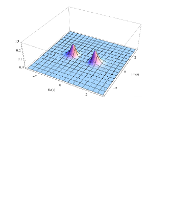
Figure 11: (color online) A plot of the spin $Q_{q}$ function of the qubits at the time $t=0$ for a state in the basin of attraction. The value of $a=0$ and we see a perfect Schrödinger cat state of the qubits. The number of qubits for the plot is $N_{q}=40$ with $\theta=0$, but a similar picture can be produced for any $N_{q}>3$. The peaks merge together for $N_{q}\leq 3$.

The ‘attractor’ states for $N_{q}$ qubits in Eq. (IV.1) are also spin coherent states (see appendix A).

$${\left|\psi^{\pm}_{N_{q}\,att}\right\rangle} = \frac{1}{\sqrt{2^{N_{q}}}}\left(e^{-i\theta}{\left|e\right\rangle}\pm i{\left|g\right\rangle}\right)\otimes...\otimes\left(e^{-i\theta}{\left|e\right\rangle}\pm i{\left|g\right\rangle}\right)$$ (59)

$$= \frac{1}{\sqrt{2^{N_{q}}}}\left(e^{-i\theta}{\left|e\right\rangle}\pm i{\left|g\right\rangle}\right)^{\otimes N_{q}}$$

$$= {\left|z=\pm ie^{i\theta},N_{q}\right\rangle}$$

In Fig 12 we plot a spin $Q_{q}$ function diagram for the ‘attractor’ state.

Figure 12: (color online) A plot of the spin $Q_{q}$ function of the qubits at the time $t=t_{r}/80$, the ‘attractor’ time when $N_{q}=40$. The initial value of $a=0$ and we see a spin coherent state centered around the value $z=ie^{i\theta}$ with $\theta=0$.

So far we have shown, for large $\bar{n}$, that the qubit states in the basin of attraction are spin Schrödinger cat states when $a\neq{\textstyle\frac{1}{\sqrt{2^{N_{q}}}}}$. At a later time, $t={\textstyle\frac{t_{r}}{2N_{q}}}$, the qubits are in the spin coherent ‘attractor’ state and the field is in a Schrödinger cat state. Then the qubits return once again to a spin Schrödinger cat state at the time $t={\textstyle\frac{t_{r}}{N_{q}}}$. This is shown in Table 2.

	$t=0$	$t=t_{r}/2N_{q}$	$t=t_{r}/N_{q}$
Field	Coherent State	Schrödinger cat state	Coherent State
Qubit	Spin Schrödinger cat state	Spin Coherent State	Spin Schrödinger cat state

Table 2: A table of the states of the field and qubits at different times. The behavior repeats in the large $\bar{n}$ approximation.

So we conclude that the ‘Schrödinger cat’ state migrates from the qubits to the field and back again.

IV.3 Collapse and Revival of Entanglement

Whilst the basin of attraction for the $N_{q}$ qubit case is a very small part of the Hilbert space of all initial states it shows many different degrees of entanglement, just like the two qubit case. Some values of $a$ and $\phi$ give the qubit state to be in a product state and other values give some degree of entanglement between the qubits. When considering more than two qubits there is no universally accepted measure of entanglement. Indeed, for $N_{q}\geq 4$ and multilevel systems there exist infinitely many inequivalent kinds of entanglement M. B. Plenio and S. Virmani (2007). GHZ type entanglement exists for all numbers of qubits and, up to local unitaries, a maximally entangled GHZ state has the form:

$${\left|GHZ\right\rangle}={\textstyle\frac{1}{\sqrt{2}}}\left({\left|b\right\rangle}^{\otimes N_{q}}+{\left|b_{\bot}\right\rangle}^{\otimes N_{q}}\right)$$ (60)

where ${\left\langle b|b_{\bot}\right\rangle}=0$. In the previous section it was stated that the basin of attraction can be rewritten as a spin ‘Schrödinger cat’ state which is a state that is a superposition of two macroscopically distinguishable states. However expanding states in the basin of attraction using Eq. (55) we see that it has a GHZ form:

$${\left|\psi_{N_{q}}\right\rangle} = \frac{1}{2}\left(\left(a+\sqrt{\frac{1}{2^{N_{q}-1}}-{{\left|a\right|}}^{2}}\right)\left({\left|e\right\rangle}+e^{-i\theta}{\left|g\right\rangle}\right)^{\otimes N_{q}}+\left(a-\sqrt{\frac{1}{2^{N_{q}-1}}-{{\left|a\right|}}^{2}}\right)\left({\left|e\right\rangle}-e^{-i\theta}{\left|g\right\rangle}\right)^{\otimes N_{q}}\right)$$

although it is only a maximal GHZ state when $a=0$ and $a={\textstyle\frac{1}{\sqrt{2^{N_{q}-1}}}}$. Excluding the case when $a={\textstyle\frac{1}{2^{N_{q}-1}}}$, all other values of $a$ give an entangled state of GHZ form. So, as with the previous case, there are only two values of $a$ that give a product state when in the basin of attraction, meaning all other states contain some entanglement. We next consider the case of three qubits in more detail and verify by numerical calculations that the basin of attraction for three qubits is indeed only made up of GHZ type entanglement.

For three qubits there are two different types of entanglement, GHZ D. M. Greenberger, M. A. Horne, A. Zeilinger (1989) and W W. Dür, G. Vidal, and J. I. Cirac (2000). ${\left|GHZ\right\rangle}=\frac{1}{\sqrt{2}}\left({\left|eee\right\rangle}+{\left|ggg\right\rangle}\right)$ can be regarded as a maximally entangled state, but if one of the qubits is traced out the remaining state has absolutely no entanglement present. The entanglement of ${\left|W\right\rangle}=\frac{1}{\sqrt{3}}\left({\left|eeg\right\rangle}+{\left|ege\right\rangle}+{\left|gee\right\rangle}\right)$ is maximally robust and is not so fragile to particle loss (i.e. there is still entanglement present after tracing out any individual qubit). It is not possible to transform ${\left|GHZ\right\rangle}$ into ${\left|W\right\rangle}$ even with a small probability of success and vise versa, and thus the two states represent fundamentally different types of entanglement. In particular, the GHZ state represents a truly 3-body entanglement. Similarly, any $N_{q}$-qubit GHZ state contains specifically $N_{q}$-body entanglement.

We have used a pure state GHZ entanglement measure introduced by Coffman et al. V. Coffman, J. Kundu and W. K. Wootters (2000):

$$\tau_{ABC}=C^{2}_{A(BC)}-C^{2}_{AC}-C^{2}_{AB}$$ (62)

where $\tau_{ABC}$ is the amount of GHZ entanglement, $C^{2}_{A(BC)}=2\sqrt{det\rho_{A}}$ and $C^{2}_{AC}$ is the entanglement after qubit B has been traced out. The results for different values of $a$ for the three qubit version of Eq. (IV.1) are shown in Fig. 13. This measurement only works for three qubit states that are pure, so we only perform the calculation on the initial state.

Figure 13: (color online) The value of the tangle for the states in the basin of attraction for different values of $a$. We notice that the plot shows only two points where the tangle is zero, just like the two qubit case.

This plot shows the same shape as that of Fig. 6, but values of $a$ are now limited to a smaller range. On the basis of Figs. 6 and 13, and using Eq. (IV.3), we conjecture that for more qubits the basin of attraction will always contain maximally entangled states that involve all the qubits and two unentangled states, but the size of the basin will get smaller as the number of qubits increases.

For the large $\bar{n}$ approximation it was shown in Sec. III.2 that if a state is started in the basin of attraction $\tau(0)=\tau({\textstyle\frac{t_{r}}{4}})$. This can also be extended to the three qubit case and $\tau_{ABC}(0)=\tau_{ABC}({\textstyle\frac{t_{r}}{6}})$. Therefore if the initial qubit state is in the basin of attraction and $\tau_{ABC}\neq 0$ then the whole entanglement will return to the qubit system at $t={\textstyle\frac{t_{r}}{6}}$.

To see if ‘Collapse and Revival’ of entanglement also occurs in the exact solution for three qubits we start the qubits in an initial state, ${\left|\psi_{3}\right\rangle}$, that is a maximally entangled GHZ state ($\tau_{ABC}=1$). We then calculated the probability $P_{init}(t)={\left\langle\psi_{3}\right|}\rho_{q}(t){\left|\psi_{3}\right\rangle}$, which is the probability the qubits are in the initial state. If the probability collapses and revives over time then we can conclude that the three qubit system also exhibits ‘Collapse and Revival’ of entanglement. The results are shown in Fig. 14. The measure stated in Eq. 62 can not be used here as the qubits are mostly in a mixed state and Eq. 62 is for a pure state. For this reason we have chosen to look at the probability of being in the initial state.

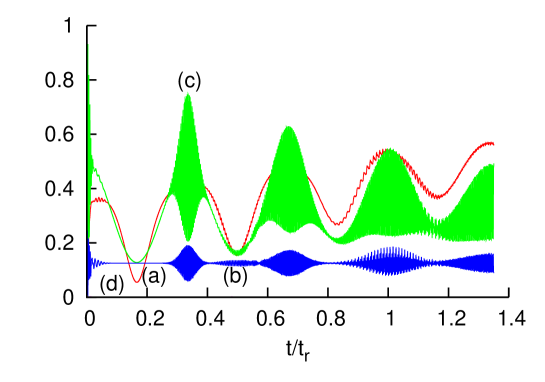
Figure 14: (color online) ‘Collapse and Revival of Entanglement’ for three qubits for the initial state, $\frac{1}{2}\left(\sqrt{3}{\left|m=1/2\right\rangle}+{\left|m=-3/2\right\rangle}\right)$, which is inside the basin of attraction, with $\bar{n}=50$ and $\theta=0$. (a) the entropy of the qubits. (b) the probability of all the qubits being in the state ${\left|g\right\rangle}$. (c) the probability of being in the initial state, $P_{init}(t)$. (d) the value of tangle when one qubit has been traced out. In fact this pink line remains zero for all time, so there is no $W$ state entanglement present.

The qubits are started in a maximally entangled GHZ state, ($\tau_{ABC}=1$), that lies in the basin of attraction and are then allowed to evolve. At a later time the entropy goes close to zero and the qubits are close to the product form shown in Eq. (47). This is a completely unentangled state and as the entropy is also zero in the large $\bar{n}$ approximation, there is no entanglement in the entire system. After the ‘attractor’ time the entropy increases and is no longer close to zero. We follow the green curve in Fig. 14 and note that $P_{init}(t)$ increases to a value near 0.8 and therefore we propose there is some three qubit mixed state entanglement present in the qubit system. In the large $\bar{n}$ approximation this value does go to unity, so the system is in the initial state, up to a phase. In this approximation we will therefore necessarily get a full revival of three-body GHZ entanglement.

As further confirmation that the entanglement is of 3-body form, we have also calculated the entanglement present between just two of the qubits after tracing out one of the qubits. It was found that the tangle between any two qubits remained zero throughout the evolution. Therefore we can conclude the entanglement present is just GHZ entanglement and there is no W component present (as a W component would lead to non-zero 2-qubit entanglement).

We have demonstrated the revival of entanglement for the numerically evaluated exact solution for two and three qubits, and shown it to be true for all values of $N_{q}$ in the large $\bar{n}$ approximation. Of particular note is that the type of entanglement we observe is of the GHZ form and is thus a true $N_{q}$-qubit entanglement that cannot be reduced to a simpler form. Remarkably, this implies that the quantum information encoded in an $N_{q}$-qubit GHZ entangled state—for any value of $N_{q}$—can be encoded into the state of a single field mode.

V Conclusion

We have studied the ‘Collapse and Revival of Entanglement’ in the two, three and many qubit JCM. We have shown that the idea of an ‘attractor’ state discovered by Gea-Banacloche J. Gea-Banacloche (1990) for one qubit does indeed exist in the multi qubit cases described by the Tavis-Cummings model. Unlike the one qubit case, the qubits have to be within a basin of attraction in order for the qubit system to disentangle itself from the field at certain times. When the qubits are started in a state in the basin of attraction then the system behaves in a similar way to the one qubit case.

The basin of attraction contains mostly entangled states and there are some interesting entanglement properties associated with the whole system when the qubits are started in this basin of attraction. The system evolves and there is then entanglement between the field and the qubit system, but when the system goes to the ‘attractor’ state all entanglement has completely left the system. The field and the qubits are both in pure states with the qubit state being in the completely unentangled ‘attractor’ state. At a later time it has been found that the entanglement does return to the system and then the process repeats. We represented explicit examples of entanglement present between the qubits and also between the qubit system and the field. We have called this phenomenon ‘Collapse and Revival of Entanglement’. For initial qubit states outside the basin of attraction, sudden death and rebirth J. H. Eberly and Ting Yu (2007) of entanglement can occur.

Appendix A Spin Coherent States

There exist spin states analogous to the coherent state of the harmonic oscillator. For the one dimensional harmonic oscillator the coherent states are functions of a variable $\alpha$ which runs over the entire complex plane:

$${\left|\alpha\right\rangle} = \frac{1}{\cal{N}}e^{\alpha a^{\dagger}}{\left|0\right\rangle}$$ (63)

$$= \frac{1}{\cal{N}}\sum_{n=0}^{\infty}\frac{(\alpha a^{\dagger})^{n}}{n!}{\left|0\right\rangle}$$ (64)

$$= e^{-{\left|\alpha\right|}^{2}/2}\sum_{n=0}^{\infty}\frac{\alpha^{n}}{\sqrt{n!}}{\left|n\right\rangle}$$ (65)

where the normalisation factor $\cal{N}$ $=e^{{\left|\alpha\right|}^{2}/2}$.

These states from a complete set, in the sense that C. C. Gerry and P. L. Knight (2005)

$$\frac{1}{\pi}\int{\left|\alpha\right\rangle}{\left\langle\alpha\right|}d^{2}\alpha=\sum_{n=0}^{\infty}{\left|n\right\rangle}{\left\langle n\right|}=\bf{1}$$ (66)

where the right hand side is the unit matrix, or identity operator.

To find the analogue for spin half particles we consider a single particle of spin $S=N_{q}/2$. We define the ground state ${\left|0\right\rangle}$ as the state such that $\hat{S}^{z}=S{\left|0\right\rangle}$ where $\hat{S}^{z}=\sum_{i=0}^{N_{q}}\sigma^{z}_{i}$ is the operator of the $z$ component of spin. Then the operator $\hat{S}^{+}=\frac{\hat{S}^{x}+i\hat{S}^{y}}{2}$ creates spin deviations. In a similar way to the field coherent state the spin coherent state for many spin half particles is J. M. Radcliffe (1971); F. T. Arecchi, E. Courtens, R. Gilmore and H. Thomas (1972); W.-M. Zhang, Da H. Feng and Gilmore (1990):

$${\left|z,N_{q}\right\rangle} = \frac{1}{\cal{N}}e^{zS^{+}}{\left|0\right\rangle}$$ (67)

$$= \frac{1}{\cal{N}}\sum_{n=0}^{N_{q}}\frac{(zS^{+})^{n}}{n!}{\left|0\right\rangle}$$ (68)

$$= \frac{1}{(1+{\left|z\right|}^{2})^{N_{q}/2}}\sum_{m=-N_{q}/2}^{N_{q}/2}\sqrt{\frac{N_{q}!}{(\frac{N_{q}}{2}-m)!(\frac{N_{q}}{2}+m)!}}z^{(\frac{N_{q}}{2}-m)}{\left|N_{q},m\right\rangle}$$ (69)

where the normalisation factor $\cal{N}$ $=\frac{1}{(1+{\left|z\right|}^{2})^{N_{q}/2}}$, $m={\textstyle\frac{N_{e}-N_{g}}{2}}$ is the spin of the state and $z$ is a complex number that determines the center of the coherent state. A spin coherent state is a product state and therefore has no entanglement. For example if $z=1$, then the average value of the spin coherent state is ${\left|N_{q},m=0\right\rangle}$, if $z=0$ then the average value of the spin coherent state is ${\left|N_{q},m={\textstyle\frac{N_{q}}{2}}\right\rangle}$ and if $z=\infty$ then the average value of the spin coherent state is ${\left|N_{q},m=-{\textstyle\frac{N_{q}}{2}}\right\rangle}$.

The states ${\left|z,N_{q}\right\rangle}$ form a complete set and the completeness relation is:

$$\frac{N_{q}+1}{\pi}\int\frac{{\left|z\right\rangle}{\left\langle z\right|}}{(1+{\left|z\right|}^{2})^{2}}d^{2}z=\sum_{m=-N_{q}/2}^{N_{q}/2}{\left|N_{q},m\right\rangle}{\left\langle N_{q},m\right|}=\bf{1}$$ (70)

In our work we present the ‘attractor’ states for many qubits in Eq. 59 as spin coherent states. These states themselves are indeed spin coherent states. If we set $z=ie^{i\theta}$ in Eq. 69 then we get ${\left|\psi^{+}_{N_{q}\,att}\right\rangle}$ and if we set $z=-ie^{i\theta}$ then we get ${\left|\psi^{-}_{N_{q}\,att}\right\rangle}$.

When looking at the coherent state of a harmonic oscillator, there exists a set of states called Schrödinger cat states that are the addition of two coherent states that are macroscopically different, e.g. ${\textstyle\frac{1}{\sqrt{2}}}({\left|\alpha\right\rangle}+{\left|-\alpha\right\rangle})$. There also exist spin coherent states that are analogous to these Schrödinger cat states. They are also defined as the addition of two macroscopically different states, i.e. ${\textstyle\frac{1}{\sqrt{2}}}({\left|z,N_{q}\right\rangle}+{\left|-z,N_{q}\right\rangle})$.

In our work we have plotted $Q$ function diagrams for the cavity field state using the coherent state. There also exists an analogous function for the qubits, defined in terms of spin coherent states in a similar way, using the completeness relation Eq. 70. This spin $Q$ function is given by

$$Q_{q}(z,t)=\frac{{\left\langle z\right|}\rho_{q}(t){\left|z\right\rangle}}{\left(1+{\left|z\right|}^{2}\right)^{2}}\;.$$ (71)

We have used this in our analysis to make interesting plots which demonstrate pictorially that the states in the basin of attraction for multi-qubit systems are indeed Schrödinger cat states of the qubits.