Quantum contributions in the ice phases: the path to a new empirical model for water – TIP4PQ/2005

Abstract

With a view to a better understanding of the influence of atomic quantum delocalisation effects on the phase behaviour of water, path integral simulations have been undertaken for almost all of the known ice phases using the TIP4P/2005 model, in conjunction with the rigid rotor propagator proposed by Müser and Berne [Phys. Rev. Lett. 77, 2638 (1996)]. The quantum contributions then being known, a new empirical model of water is developed (TIP4PQ/2005) which reproduces, to a good degree, a number of the physical properties of the ice phases, for example densities, structure and relative stabilities.

I Introduction

“Water, water, every where…” goes the poet Samuel Taylor Coleridge’s The Rime of the Ancient Mariner, which provides a magnificent résumé of our reason for studying this ubiquitous material. Many volumes have been written about water and ice (to cite just a few Eisenberg and Kauzmann (1969); Petrenko and Whitworth (1999); Franks (2000); Ball (2001); boo (2009)), and a good deal more await writing, before we fully understand this enigmatic molecule.

Currently the point has been reached where many properties, including the global phase diagram of water and the ice phases, can be reproduced qualitatively (and in some cases, quantitatively) using little more than a simple empirical model Sanz et al. (2004). However, there are several aspects of water where our knowledge, and thus our understanding, is far from complete. One such aspect is the high pressure/temperature region of the phase diagram, where the precise location of the melting curves is still yet to be agreed upon due to the difficult nature of the experiments. For example, it is an open question as to whether water becomes super-ionic in this region Goncharov et al. (2005); Schwegler et al. (2008). In one of the ice polymorphs, ice X, the notion of a water molecule even becomes lost, the protons being shared equally between oxygen atoms Benoit et al. (1998); Loubeyre et al. (1999). The low temperature region of the phase diagram is also extremely interesting, where a host of ‘anomalous’ or atypical trends are also present. Examples are the well known maximum in density at 3.984 Celsius, a minimum in the isothermal compressibility at 46.5 Celsius, and an unusual variation of the diffusion coefficient with pressure. These trends are especially apparent in super-cooled water where one can also find a minimum in both the density Liu et al. (2007) and a dynamic transition to Arrhenius behaviour for the diffusion coefficient Xu et al. (2005); Kumar et al. (2007). It has been suggested that many of the anomalous properties of water at low temperatures could be understood by an hypothesised second critical point Poole et al. (1992); Debenedetti and Stanley (2003); Debenedetti (2003) buried deep within “no-mans land” Stanley et al. (2000), a region of the phase diagram inaccessible to experiment. If this is so, it would go a long way to explaining another feature of water; its capacity to form several amorphous phases (glasses) at low temperatures.

In elucidating the origin of these anomalies, computer simulations have played a prominent role, for example their part in the proposal of a second critical point in water Poole et al. (1992); Stanley et al. (1994) using a simple empirical model. Classical computer simulations do, however, have their limitations. There are certain systems, water being one of them, where quantum effects are significant Morrone and Car (2008); Paesani and Voth (2009). As an example, let us examine the difference in temperature between the melting point and the temperature of maximum density. For H₂O this amounts to 3.984K, whereas for D₂O it is 7.365K. From the point of view of the Born-Oppenheimer approximation the potential energy surface (PES) is independent of the isotope considered. Thus the different behaviour of these isotopes is due to how the molecules react to this PES. This is known as an atomic quantum delocalisation effect. In this particular case the origin of the differences, both structural and dynamical, is in good part due to the quantum nature of the hydrogen protons and the strength of the hydrogen bond. Another example is the self-diffusion coefficient, which increases by more than 50% in a quantum system with respect to classical molecular dynamics simulations de la Peña and Kusalik (2006); Miller and Manolopoulos (2005).

The overall structure of water is that of an asymmetric top, which is to say that all three principal moments of inertia are distinct. What is particularly interesting is that since hydrogen is the lightest atom, the rotational moments of inertia are small enough to show marked quantum behaviour. Thus water has significant quantum effects even at room temperature. The importance of these quantum effects increases as the temperature is lowered. For the ice phases these effects are expected to be significant, especially at 77K where many experiments on ice are frequently performed using liquid nitrogen. Thus far there has been relatively little work on these effects for ice, and almost all of the work that has been published has focused on ice I_h Gai et al. (1996); de la Peña et al. (2005); de la Peña and Kusalik (2006); Paesani and Voth (2008). The objective of this publication is to quantify the size of these effects in all of the ice phases, apart from that of ice X, which cannot be described by the rigid models used in this work.

These atomic quantum delocalisation effects will be studied using the empirical TIP4P/2005 model Abascal and Vega (2005). Over the last few years a number of the present authors have undertaken extensive simulation studies examining the performance of a number of commonly used models for water, in particular the TIP3P, TIP4P, TIP5P and SPC/E models Vega et al. (2009). The principal findings have been that the TIP3P Jorgensen et al. (1983), TIP5P Mahoney and Jorgensen (2000) and SPC/E Berendsen et al. (1987) models experience difficulties when it comes to describing the global phase diagram of water and the ice phases. However, the TIP4P model does indeed provide a qualitatively correct phase diagram. Based on this finding, the TIP4P model was re-parameterised in order to improve the quantitative representation, leading to the TIP4P/2005 model Abascal et al. (2009). It has since been found that this model also provides a good description of the maximum in density of liquid water and its variation with pressure Pi et al. (2009), of the compressibility minima Pi et al. (2009), the surface tension Vega and de Miguel (2007), the vapour liquid equilibria Vega et al. (2006), the critical properties Vega et al. (2006), the equation of state at high pressures Vega et al. (2009), the diffusion coefficient Vega et al. (2009), and the viscosity Vega et al. (2009).

That said, the model was parameterised for classical simulations, so the introduction of atomic quantum delocalisation effects, although improving the qualitative description, will cause a deterioration in the quantitative description. In the first stage of this research we shall analyse the impact of atomic quantum delocalisation effects on the properties of the ice phases using this potential. That will elucidate where, and how, atomic quantum delocalisation effects modify the properties of water with respect to the classical limit. These differences then known, we provide a re-parameterised version of the TIP4P/2005 model which we shall call the TIP4PQ/2005 model, the Q indicating that this model is suitable for quantum simulations. As was pointed out by Morse and Rice Morse and Rice (1982) as well as by Whalley “…effective potentials that are used to simulate water ought to be tested on the many phases of ice before being treated as serious representations of liquid water” Whalley (1984).

II Methodology

Simulations were performed using the path integral formulation, which permits us to study the quantum effects related to the finite mass of the atoms (in many quantum chemistry calculations, the electrons are treated as being quantum, however the nuclei are treated as classical point masses). A particularly elegant technique for studying quantum effects in many body systems is that of path-integral Monte Carlo (PIMC). There are many good introductions concerning PIMC in the literature Feynman and Hibbs (1965); Chandler and Wolynes (1981); Gillan (1990); Ceperley (1995); Allen and Tildesley (1987), here we shall focus on the aspects most pertinent to the simulations we have performed.

Water is, of course, a flexible molecule. For path integral simulations one generally requires the number of Trotter slices, $P$, to be Markland and Manolopoulos (2008)

$$P>\frac{\hbar\omega_{\mathrm{max}}}{k_{B}T}$$ (1)

where $\omega_{\mathrm{max}}$ is the ‘fastest’ frequency present in the system in question. In water the intramolecular vibrations are of the order of $\omega_{\mathrm{max}}/2\pi c\approx 4000~{}\mathrm{cm}^{-1}$ which leads to $P>20$. Using the rigid body approximation for water the fastest motion now becomes the libration, with a frequency of $<900~{}\mathrm{cm}^{-1}$, thus reducing $P$ to around 5-6. This represents a substantial reduction in the computational overhead associated with traditional PIMC calculations (although new techniques have recently been developed by Manolopoulos et al. to increase the efficiency of flexible molecule PIMC Markland and Manolopoulos (2008)). It must be said that by choosing to use a rigid model, one precludes the ability to study some aspects of water, such as the high frequency region of the infra-red adsorption spectrum Poulsen et al. (2005); Habershon et al. (2008). The infra-red spectrum of water and ice can be divided up into two distinct regions. Above $\approx 900~{}\mathrm{cm}^{-1}$ one has the contribution associated with the intramolecular degrees of freedom of bending and stretching. Below $\approx 900~{}\mathrm{cm}^{-1}$, as previously mentioned, one has the section that corresponds to translational and librational movements, and are mostly due to inter-molecular forces. Quantum contributions to the Helmholtz energy $(A)$ within a perturbative treatment for a rigid asymmetric top are given by Powles and Rickayzen (1979):

$$\frac{A-A_{C1}}{N_{m}}=\frac{\hbar^{2}}{24(k_{B}T)^{2}}\left[\frac{\left<F^{2}\right>}{M}+\frac{\left<\Gamma_{A}^{2}\right>}{I_{A}}+\frac{\left<\Gamma_{B}^{2}\right>}{I_{B}}+\frac{\left<\Gamma_{C}^{2}\right>}{I_{C}}\right]-\frac{\hbar^{2}}{24}\sum_{\mathrm{cyclic}}\left(\frac{2}{I_{A}}-\frac{I_{A}}{I_{B}I_{C}}\right)+{\mathcal{O}}(\hbar^{4})$$ (2)

A good proportion of the quantum effects in water are due to the strength of the hydrogen bond, along with a particularly small inertia tensor. It is this that lends importance to the torque $(\Gamma)$ terms found in the above equation, which results in the appearance of the librational band. In contrast, this region for a molecule such as SO₂, where no such hydrogen bonding is present, is far less important. By using the path integral formulation for a rigid model we shall be studying atomic quantum delocalisation effects in the influential region encountered below $\approx 900~{}\mathrm{cm}^{-1}$. In a study of the phonon density of states for ice I_h Dong and Li Dong and Li (200) showed that the rigid TIP4P model does a reasonable job of reproducing this low frequency section of the spectrum. Even given the fact that intramolecular effects are important, it is surely the case that a rigid body path-integral study is more physically realistic than a purely classical study, which neglects all atomic quantum delocalisation effects. Such an approach has been adopted in a number of studies, using for example the SPC/E model Miller and Manolopoulos (2005). In view of this, and given the success that the TIP4P/2005 model has had in describing the ice phases classically, the rigid TIP4P/2005 model is the natural candidate for a preliminary study of atomic quantum delocalisation effects in ices. Given that the TIP4P/2005 model is a rigid asymmetric top, we shall first present the path integral description of a rigid rotor.

II.1 Path integrals for a rigid molecule

The coordinates used to describe a rigid molecule are $\mathbf{r}_{1}\mathbf{\Omega}_{1}$, where $\mathbf{r}_{1}$ represents the centre of mass and $\mathbf{\Omega}_{1}=(\phi_{1},\theta_{1},\chi_{1})$ represents the Euler angles that fix the molecule orientation. The Hamiltonian of a rigid asymmetric rotor can be written in the form Marx and Müser (1999):

$$\hat{H}_{1}=\hat{T}^{\mathrm{tra}}+\hat{T}^{\mathrm{rot}}+\hat{U}\,,$$ (3)

where $\hat{T}^{\mathrm{tra}}$ represents the kinetic energy operator associated to the centre of mass translation, $\hat{U}$ appears as a potential energy operator that is a function of the coordinates $\mathbf{r}_{1}\mathbf{\Omega}_{1}$, and the rotational kinetic energy operator is given by Marx and Müser (1999):

$$\hat{T}^{\mathrm{rot}}=\sum_{i=1}^{3}\frac{\hat{L}_{i}^{2}}{2I_{i}}\,,$$ (4)

where $\hat{L}_{i}$ are the components of the angular momentum operator and $I_{i}$ are the moments of inertia of the molecule referred to its fixed body frame. We assume, without loss of generality, that the moment of inertia tensor is diagonal in the chosen fixed body frame.

In the path integral formulation, the partition function, $Q_{1}$, of a rigid molecule may be expressed by a factorisation of the density matrix into $P$ factors, so that each quantum particle is described by a ring of $P$ replicas or ‘beads’,

$$Q_{1}(\beta) = \lim_{P\rightarrow\infty}\int\ldots\int\prod_{t=1}^{P}\mathrm{d}\mathbf{r}_{1}^{t}\mathrm{d}\mathbf{\Omega}_{1}^{t}\prod_{t=1}^{P}\rho_{1}^{t,t+1}(\beta/P)\,,$$ (5)

where $\beta=1/k_{B}T$ is the inverse temperature, and the propagator $\rho_{1}^{t,t+1}$ is approximated by Marx and Müser (1999):

$$\rho_{1}^{t,t+1}(\beta/P)\approx\left<\mathbf{r}_{1}^{t}\mathbf{\Omega}_{1}^{t}|\exp\left[-\beta\hat{U}/2P\right]\exp\left[-\beta(\hat{T}^{\mathrm{tra}}+\hat{T}^{\mathrm{rot}})/P\right]\exp\left[-\beta\hat{U}/2P\right]|\mathbf{r}_{1}^{t+1}\mathbf{\Omega}_{1}^{t+1}\right>.$$ (6)

The propagator satisfies the cyclic condition that bead $P+1$ corresponds to bead $1$. This rigid molecule propagator is built up of three factors, a potential energy component, a translational component, and a rotational component:

$$\rho_{1}^{t,t+1}(\beta/P)\approx\rho^{t,t+1}_{\mathrm{pot},1}\rho^{t,t+1}_{\mathrm{tra},1}\rho^{t,t+1}_{\mathrm{rot},1}.$$ (7)

The potential energy component is given by Marx and Müser (1999)

$$\rho^{t,t+1}_{\mathrm{pot},1}=\exp\left[-\frac{\beta}{2P}\left(U^{t}+U^{t+1}\right)\right]\,,$$ (8)

where $U^{t}=U(\mathbf{r}_{1}^{t}{\bf\Omega}_{1}^{t})$ is the potential energy of the replica $t$ of the molecule. The translational component is given by Marx and Müser (1999)

$$\rho^{t,t+1}_{\mathrm{tra},1}=\left<\mathbf{r}_{1}^{t}|\exp\left(-\beta\hat{T}^{\mathrm{tra}}/P\right)|\mathbf{r}_{1}^{t+1}\right>=\left(\frac{MP}{2\pi\hbar^{2}\beta}\right)^{3/2}\exp\left[-\frac{MP}{2\hbar^{2}\beta}(\mathbf{r}_{1}^{t}-\mathbf{r}_{1}^{t+1})^{2}\right],$$ (9)

where $M$ is the total mass of the rigid molecule. The two previous equations are well known and are commonly used as the so-called primitive approximation in path integral studies of simple fluids. The rotational propagator between $t$ and $t+1$ is given by Marx and Müser (1999):

$$\rho^{t,t+1}_{\mathrm{rot},1}=\left<{\bf\Omega}_{1}^{t}|\exp\left[-\beta\hat{T}^{\mathrm{rot}}/P\right]|{\bf\Omega}_{1}^{t+1}\right>.$$ (10)

In an important piece of work Müser and Berne Marx and Müser (1999); Müser and Berne (1996) have shown that the rotational contribution to the propagator between the replicas $t$ and $t+1$ of a rigid molecule $i$ is exactly given by

$$\rho_{{\mathrm{rot}},i}^{t,t+1}(\tilde{\theta}_{i}^{t,t+1},\tilde{\phi}_{i}^{t,t+1}+\tilde{\chi}_{i}^{t,t+1})=\sum_{J=0}^{\infty}\sum_{M=-J}^{J}\sum_{\tilde{K}=-J}^{J}f_{i,J,M,\tilde{K}}^{t,t+1}\exp\left(-\frac{\beta E^{JM}_{\tilde{K}}}{P}\right)$$ (11)

where

$$f_{i,J,M,\tilde{K}}^{t,t+1}=\frac{2J+1}{8\pi^{2}}d^{J}_{MM}(\tilde{\theta}_{i}^{t,t+1})\cos[M(\tilde{\phi}_{i}^{t,t+1}+\tilde{\chi}_{i}^{t,t+1})]|A_{\tilde{K}M}^{(JM)}|^{2}$$ (12)

Here $d^{J}_{MM}(\tilde{\theta}_{i}^{t,t+1})$ are Wigner functions and $|A_{\tilde{K}M}^{(JM)}|$ are the coefficients of the expansion of the eigenstates of the asymmetric top in a basis formed by the eigenstates of the symmetric top. $E_{\tilde{K}}^{(JM)}$ are the eigenvalues of the energy of the asymmetric top. The quantum numbers $J$ and $M$ provide the values of the total angular momenta of the asymmetric top and the value of its $z$ component in the laboratory frame. The number $\tilde{K}$ is not a true quantum number, in the sense that it does not provide the value of any physical observable, but rather is an index used to label the $(2J+1)$ energy levels that are obtained for each value of $J$. The angles $\tilde{\theta}^{t,t+1}_{i}$, $\tilde{\phi}^{t,t+1}_{i}$ and $\tilde{\chi}^{t,t+1}_{i}$ are the Euler angles of the replica $t+1$ of molecule $i$ expressed in the body frame fixed in the replica $t$ of the same molecule $i$. Note that the rotational propagator depends solely on two variables, $\tilde{\theta}^{t,t+1}_{i}$ and $\tilde{\phi}^{t,t+1}_{i}+\tilde{\chi}_{i}^{t,t+1}$. Obviously to determine the value of the rotational propagator one must first determine the $(2J+1)$ energy levels of the asymmetric top for each value of $J$. This can be obtained from the $(2J+1)$ eigen-values, $E_{\tilde{K}}^{(JM)}$, of the matrix given in Ref. Zare, 1988. The coefficients $|A_{\tilde{K}M}^{(JM)}|$ are the eigen-vectors associated with these eigen-values. It is computationally convenient to calculate the rotational propagator $\rho_{{\mathrm{rot}},i}^{t,t+1}(\tilde{\theta}_{i}^{t,t+1},\tilde{\phi}_{i}^{t,t+1}+\tilde{\chi}_{i}^{t,t+1})$ for a grid of values of the angles $\tilde{\theta}^{t,t+1}_{i}$ and $\tilde{\phi}^{t,t+1}_{i}+\tilde{\chi}_{i}^{t,t+1}$ for each value of $\beta/P$ to be used, and save this data prior to the simulations. The value of the rotational propagator for any given $\tilde{\theta}^{t,t+1}_{i}$ and $\tilde{\phi}^{t,t+1}_{i}+\tilde{\chi}_{i}^{t,t+1}$ can then be estimated using a linear interpolation algorithm from this tabulated data.

II.2 Path integrals for an ensemble of rigid molecules

Once the translational and rotational propagators are known for a rigid molecule one can calculate the partition function for a set of interacting molecules. Let us assume that we shall be using a pair-wise potential $u_{ij}$ such that the potential energy of the replica $t$ of the system is

$$U^{t}=\sum_{i}\sum_{j>i}u_{ij}(\mathbf{r}_{i}^{t},\mathbf{r}_{j}^{t},{\bf\Omega}_{i}^{t},{\bf\Omega}_{j}^{t}).$$ (13)

Now the canonical partition function, $Q_{N}$, of an ensemble of $N$ molecules described with $P$ beads is given by:

$$Q_{N}(\beta) \approx \frac{1}{N!}\left(\frac{MP}{2\pi\beta\hbar^{2}}\right)^{3NP/2}\int\ldots\int\prod_{i=1}^{N}\prod_{t=1}^{P}d\mathbf{r}_{i}^{t}d{\bf\Omega}_{i}^{t}\times$$ (14)

$$\exp\left(-\frac{MP}{2\beta\hbar^{2}}\sum_{i=1}^{N}\sum_{t=1}^{P}\left(\mathbf{r}_{i}^{t}-\mathbf{r}_{i}^{t+1}\right)^{2}-\frac{\beta}{P}\sum_{t=1}^{P}U^{t}\right)\prod_{i=1}^{N}\prod_{t=1}^{P}\rho_{{\mathrm{rot}},i}^{t,t+1}\,.$$

As can be seen in Eqs. (13) and (14), each replica $t$ of molecule $i$ interacts: (a) with the molecules that have the same index $t$ via the intermolecular potential $u_{ij}$; (b) with replicas $t-1$ and $t+1$ of the same molecule $i$ via a harmonic potential whose coupling parameter depends on the mass of the molecules, $M$, and on the inverse temperature $\beta$; and (c) with replicas $t-1$ and $t+1$ of the same molecule through the terms $\rho_{{\mathrm{rot}},i}^{t-1,t}$ and $\rho_{{\mathrm{rot}},i}^{t,t+1}$ which incorporate the quantisation of the rotation, which in turn depends on the relative orientation of replica $t$ with respect to $t-1$, and $t+1$ with respect to $t$.

Let us define an energy $U^{\prime}$ as:

$$U^{\prime}=\frac{MP}{2\beta^{2}\hbar^{2}}\sum_{i=1}^{N}\sum_{t=1}^{P}\left(\mathbf{r}_{i}^{t}-\mathbf{r}_{i}^{t+1}\right)^{2}+\frac{1}{P}\sum_{t=1}^{P}U^{t}\,,$$ (15)

and the total orientational propagator $P_{\mathrm{rot}}$ as:

$$P_{\mathrm{rot}}=\prod_{i=1}^{N}\prod_{t=1}^{P}\rho_{{\mathrm{rot}},i}^{t,t+1}\,.$$ (16)

Within a Monte Carlo simulation one generates a new configuration starting from a previous configuration. The probability of accepting this new configuration, $p_{accept}$, is given by

$$p_{accept}=\min\left[1,\exp\left(-\beta(U^{\prime}_{new}-U^{\prime}_{old})\right)\frac{P^{new}_{{\mathrm{rot}}}}{P^{old}_{{\mathrm{rot}}}}\right]\,.$$ (17)

It is worthwhile making two observations about the orientational propagator between a pair of contiguous beads $\rho_{{\mathrm{rot}},i}^{t,t+1}$. Firstly, it must be positive in order to be used in the Metropolis acceptance criteria, which is indeed the case. Secondly, the maximum in the orientational propagator is achieved when $\tilde{\theta}=0$ and $\tilde{\phi}+\tilde{\chi}=0$. It is found that at high enough temperature the propagator decays to zero relatively quickly as the values of $\tilde{\theta}$ and $\tilde{\phi}+\tilde{\chi}$ increase. The orientational propagator can also be expressed as an auxiliary energy by defining $u_{i,aux}$ such that

$$u_{i,aux}^{t,t+1}=-\frac{1}{\beta}\ln\rho_{{\mathrm{rot}},i}^{t,t+1}$$ (18)

$u_{i,aux}$ has a minimum at $\tilde{\theta}=0$ and $\tilde{\phi}+\tilde{\chi}=0$ and increases quickly as a function of the variables $\tilde{\theta}$ and $\tilde{\phi}+\tilde{\chi}$. $P_{\mathrm{rot}}$ can now be written as

$$P_{\mathrm{rot}}=\exp(-\beta U_{\mathrm{aux}})=\exp\left(-\beta\sum_{i=1}^{N}\sum_{t=1}^{P}u_{i,aux}^{t,t+1}\right).$$ (19)

Using this auxiliary energy the Metropolis criteria can be now written as :

$$p_{accept}=\min\left[1,\exp\left(-\beta\left((U^{\prime}_{new}+U_{\mathrm{aux},new})-(U^{\prime}_{old}+U_{\mathrm{aux},old})\right)\right)\right]\,.$$ (20)

This expression helps us to clarify the role of the orientational propagator; it can be viewed as a potential that forces two contiguous beads, $t$ and $t+1$, to adopt similar orientations (this corresponds to the minimum of the auxiliary potential) with an energetic penalty when they adopt different orientations. This is analogous to the role played by the harmonic springs connecting the centre of masses of the molecules in Eq. (15).

The internal energy can now be calculated from:

$$E=-\frac{1}{Q_{N}}\frac{\partial Q_{N}}{\partial\beta}\,.$$ (21)

It can be shown that substituting the value of the canonical partition function in this expression results in

$$E=K_{\mathrm{tra}}+K_{\mathrm{rot}}+U\,,$$ (22)

where :

$$K_{tra} = \frac{3NP}{2\beta}-\left\langle\frac{MP}{2\beta^{2}\hbar^{2}}\sum_{i=1}^{N}\sum_{t=1}^{P}({\bf r}_{i}^{t}-{\bf r}_{i}^{t+1})^{2}\right\rangle,$$

$$K_{rot} = \left\langle\frac{1}{P}\sum_{i=1}^{N}\sum_{t=1}^{P}\frac{\sum_{J=0}^{\infty}\sum_{M=-J}^{J}\sum_{\tilde{K}=-J}^{J}f_{J,M,\tilde{K}}^{i,t,t+1}{\tilde{E}}_{\tilde{K}}^{JM}\exp{\left[-\frac{\beta}{P}\tilde{E}_{\tilde{K}}^{JM}\right]}}{\rho_{rot,i}^{t,t+1}}\right\rangle,$$

$$U = \left\langle\frac{1}{P}\sum_{t=1}^{P}U^{t}\right\rangle\,.$$ (23)

As with the rotational propagator, the numerator of $K_{rot}$ in Eq. 23 was calculated prior to the simulations for a grid of the variables $\tilde{\theta}$ and $\tilde{\phi}+\tilde{\chi}$ and subsequently saved in tabular form.

When performing simulations of solids it is more convenient to perform the simulations in the $NpT$ ensemble. The partition function for the $NpT$ ensemble can be calculated using:

$$Q_{NpT}=A\int dV\exp(-\beta pV)Q_{N}$$ (24)

where $A$ is a constant with units of inverse volume that makes $Q_{NpT}$ dimensionless. Its value affects the Helmholtz energy function, but not the configurational properties.

II.3 Simulation details

In this work path integral Monte Carlo simulations are undertaken for the TIP4P/2005 model for fourteen of the fifteen known ice phases. One of the most important variables when it comes to path integral simulations is the number of Trotter slices, or beads, ($P$) employed. If $P=1$ then the simulation is classical. As $P\rightarrow\infty$ then the quantum simulation becomes exact. Given the isomorphism between Trotter slices and the number of component ‘beads’ in a ring polymer Chandler and Wolynes (1981), one can easily see that the time required for a simulation scales with the number of Trotter slices used. For flexible models of water at 300K a typical number of slices is about $P=24$ Lobaugh and Voth (1997); Stern and Berne (2001); Shinoda and Shiga (2005). However, if a rigid model is employed, the number of Trotter slices required can be reduced by about a factor of five Mahoney and Jorgensen (2001); de la Peña et al. (2005). Previous studies for a rigid model of water at 300K found that a value of $P=5$ provides good convergence Gai et al. (1996); de la Peña et al. (2005). Thus in this work the number of Trotter slices times the temperature was maintained at $PT\approx 1500$. For the lowest considered temperature (77K) this corresponds to 20 beads. When computing the asymmetric top eigen-energies and eigenvectors of water the OH distance and the H-O-H bond angle of the TIP4P/2005 model were used, which corresponds to the gas phase geometry of real water. The principal moments of inertia are computed using this geometry along with the masses of the hydrogen and oxygen atoms. Although the model has the negative charge on the site M, this site is massless and therefore it is only used to compute the potential energy of the system.

In this work two models of water are studied, the TIP4P/2005 model Abascal and Vega (2005) and a re-parameterisation, which we shall call the TIP4PQ/2005 model, to ‘compensate’ for quantum effects. The parameters for both of these models are given in Table 1. The only difference between these models is an increase in the charges on the hydrogen sites by 0.02e, along with a corresponding increase in the charge on the oxygen site. For both models the Lennard-Jones potential was truncated at 8.5Å and long-range corrections were included. The TIP4P/2005 model has been designed to be used with Ewald summations de Leeuw et al. (1980a, b) which is a well known technique to treat the long range electrostatic interactions. Ewald summation is more appropriate than the reaction field method when it comes to the simulation of solid phases. The real part of the Coulombic potential was truncated at 8.5Å.

The configurational space of the quantum system was sampled using a Monte Carlo code with four distinct types of trial moves: the displacement of a single bead of one molecule, rotation of a single bead of one molecule, translation of a whole ring, and rotation of all of the replicas of one molecule. A Monte Carlo cycle is defined as $N$ Monte Carlo moves, where the probability of attempting a translation or a rotation of a single bead is 30% each and the probability of attempting a translation of a whole ring or rotating all the replicas of a ring is 20% each. The maximum displacement or rotation in each type of movement was adjusted to obtain a 40% acceptance probability. When simulations were performed in the $NpT$ ensemble, besides the $N$ particle trial moves, one Monte Carlo cycle also includes an attempt to change the volume of the simulation box. The maximum volume change was adjusted so as to obtain a 30% acceptance probability. In general the simulations consisted of 30,000 Monte Carlo equilibration cycles, followed by a further 100,000 cycles for the accumulation of run averages. The number of molecules used in each of the phases are given in Table 2. For the proton disordered ice phases the positions of the hydrogen atoms were generated in such a way as to produce a system that satisfies the so-called Bernal-Fowler ice rules Bernal and Fowler (1933); Pauling (1935), and whose dipole moment as close as possible to zero. This was achieved using the algorithm proposed by Buch et al. Buch et al. (1998); MacDowell et al. (2004).

As mentioned, all simulations were performed in the isothermal-isobaric ($NpT$) ensemble. The implementation of the $NpT$ ensemble in PIMC has already been discussed in previous works Barrat et al. (1989); Müser et al. (1995). It is important to note that the Monte Carlo volume moves should be performed anisotropically, in order to allow the simulation box to ‘relax’ and obtain the true equilibrium unit cell of the model under consideration. In other words, the pressure on the simulation box should be hydrostatic; the pressure tensor is diagonal and each of the elements along the diagonal have the same value. If this is not the case the system will suffer stresses and the structure and thermodynamic properties will not reach their equilibrium values. This is achieved using the technique proposed by Parrinello and Rahman Parrinello and Rahman (1980, 1982); Najafabadi and Yip (1983) and extended to Monte Carlo by Yashonath and Rao Yashonath and Rao (1985). Briefly, the shape of the simulation box is defined by a so-called $H$-matrix representing the Cartesian coordinates of the vectors defining the simulation box. Each of the individual components of the $H$-matrix are adjusted randomly, leading to changes in both the simulation box lengths and in the geometry.

As a preliminary check that the Müser and Berne propagator was implemented correctly the rotational energies were calculated for an isolated H₂O molecule. In Fig. 1 the rotational energies computed from the exact expression of the quantum partition function of an asymmetric top Levine (1975) (with the appropriate rotational constants) are compared to those obtained from PIMC simulations. As can be seen the agreement is excellent. It should be noted that the present calculations do not include exchange effects. However, these are only expected to be relevant at temperatures below those that we have studied in this work.

III Results

A single state point has been simulated for each of the solid phases of water with the exception of ice X, which cannot be described by a rigid model Benoit et al. (1998); Loubeyre et al. (1999). The results of these simulations are presented in Table 2. By comparing the densities obtained from classical TIP4P/2005 simulations to path integral simulations of the TIP4P/2005 model, which henceforth we shall denote as TIP4P/2005_(PI), it is clear that the introduction of atomic quantum delocalisation effects reduces the density of the solid phase by about 0.02 g/cm³ for temperatures above 200K, and by $\approx 0.03-0.04$g/cm³ for temperatures in the range 75-170K. Not surprisingly, quantum effects become increasingly evident as the temperature is reduced. The various contributions to the total energy, $E$, are also tabulated. As far as the translational kinetic energy component, $K_{\mathrm{translational}}$, is concerned one can observe an increase of about 10% for TIP4P/2005_(PI) with respect to TIP4P/2005 (i.e. $(3/2)RT$) at temperatures above 225K. As the temperature is lowered, this difference becomes 100%. This is approximately true for all of the ices. From these results one can conclude that the translational contribution to the heat capacity in quantum simulations is significantly less than the corresponding contribution in classical simulations. If one looks at the rotational kinetic energy contribution, $K_{\mathrm{rotational}}$, the differences are exaggerated even further; ranging from about 100% for ‘high’ temperature ices, and increasing to 600% at low temperatures. From this it is clear that the quantum contributions are manifestly rotational in their nature, whilst translational effects are secondary in the solid phase. Within a perturbative treatment the quantum contribution to the Helmholtz energy function is related to the average of the forces divided by the masses for the translational contribution, and to the average of the torques divided by the principal moments of inertia for the orientational contribution Allen and Tildesley (1987). The mass of water is almost the same as that of neon, however, the quantum effects are far more pronounced in water for the temperature range considered in this work Ramirez and Herrero (2008). The overwhelming reason for this difference is the strength and directionality of the hydrogen bond. This, as well as the fact that the moments of the inertia tensor are quite small due to hydrogen having a very low mass. The temperature dependence of the kinetic rotational energy is rather weak, so its contribution to the heat capacity is expected to be small. On the other hand the quantum contributions to the potential energy are of the order of 1 kcal/mol at high temperatures, which increases to 1.5 kcal/mol at low temperatures. Thus there is a significant difference in $E$ between the TIP4P/2005 and the TIP4P/2005_(PI) results, amounting to about 3 kcal/mol at low temperatures; half of which being due potential energy, and the other half kinetic.

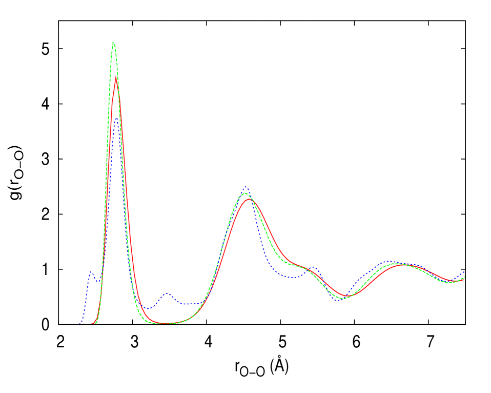
Figure 2: Radial distribution function of ice I_h for TIP4P/2005 (dashed green line) and TIP4P/2005_(PI) (solid red line) at 250 K and p=0 bar. The blue dotted line corresponds to the experimental data of Soper at 220K Soper (2000).

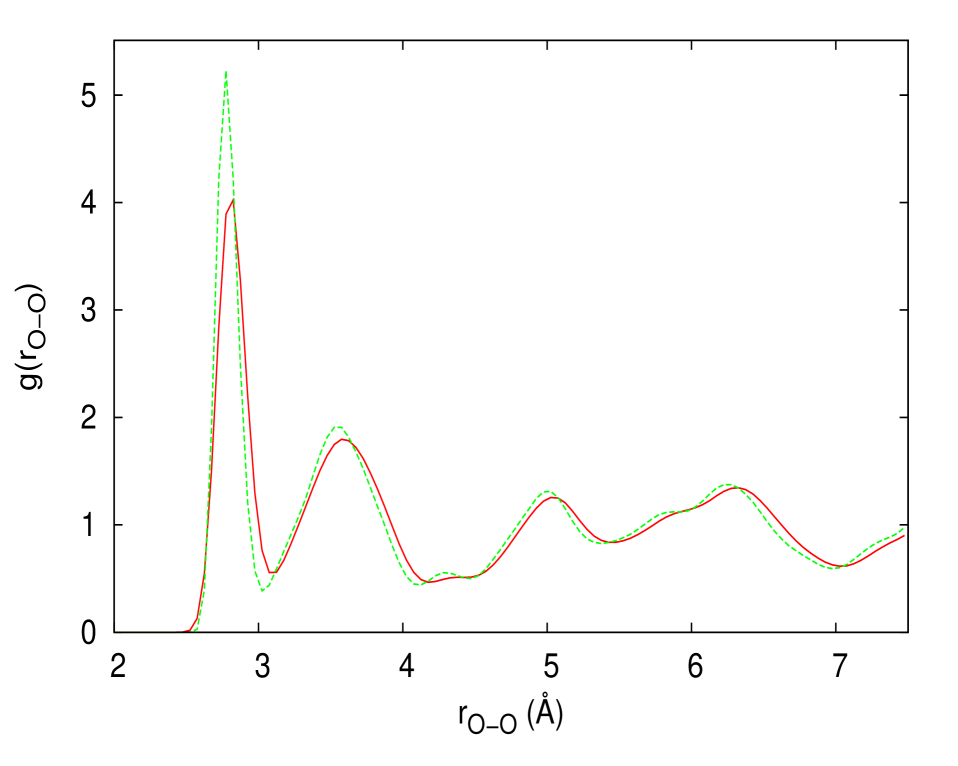
Figure 3: Radial distribution function of ice II for TIP4P/2005 (dashed green line) and TIP4P/2005_(PI) (solid red line) at 123 K and p=0 bar.

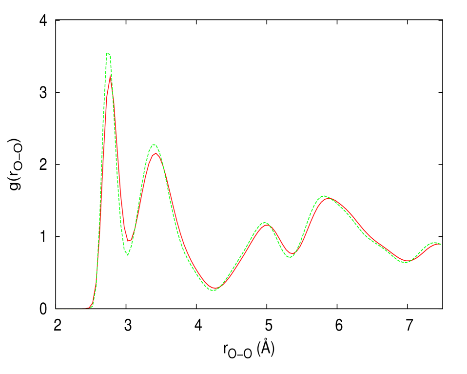
Figure 4: Radial distribution function of ice VI for TIP4P/2005 (dashed green line) and TIP4P/2005_(PI) (solid red line) at 225 K and p=11 kbar.

We shall now turn to the radial distribution functions. These histograms provide insights into the structure of a fluid on a molecular scale Whalley (1984); Vega et al. (2005). One of the first simulation studies of such functions for water using path integral simulations was undertaken by Kuharsky, Rossky and co-workers Kuharski and Rossky (1984); Kuharski and Rossky (1985a); Buono et al. (1991); Kuharski and Rossky (1985b) for the ST2 model. Given the low scattering factor of hydrogen, the oxygen-oxygen ($g_{\rm OO}$) is the distribution function most accessible experimentally. Here we present the oxygen-oxygen radial distribution function for ices I_h, II and VI (Figures 2-4) for classical TIP4P/2005 and TIP4P/2005_(PI). For ice I_h the experimental radial distribution function has also been plotted, using the data provided by Soper Soper (2000) at 220K. To the best of our knowledge as yet there are no experimental radial distribution functions available in the literature for ices II and VI. In Table 3 details are given for specific points located along the oxygen-oxygen radial distribution function curves for ice I_h. On going from classical simulations to path integral simulations the location of the first two peaks shifts to slightly larger distances. Furthermore, there is a notable reduction in the height of these peaks when quantum contributions are incorporated. Similar findings have been published previously for water and for simulations of TIP4P_(PI) of ice I_h by Hernández de la Peña et al. de la Peña et al. (2005). This softening of the distribution functions goes hand-in-hand with the reduction in the density of the ices in the PIMC calculations. It is interesting to speculate whether the addition of the small (and somewhat unusual) first peak in the ice I_h experimental data with the much larger second peak would place the simulation results in a more favourable light.

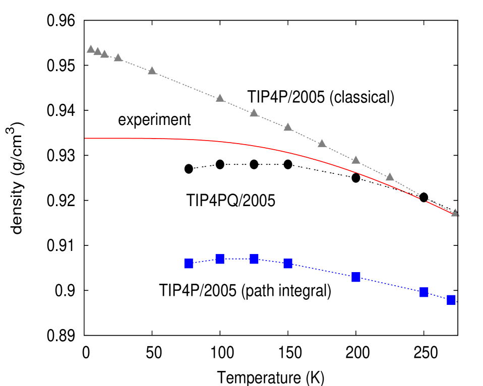
Figure 5: Equations of state for ice I_h at $p=1$ bar. Classical TIP4P/2005 model (grey dot-dashed line / filled triangles) Noya et al. (2007), experimental data (red solid line) Feistel and Wagner (2006), TIP4P/2005_(PI) (blue dotted line/ filled squares) and the new TIP4PQ/2005 model (black double-dotted line / filled circles). The error in the density is of order $\pm 0.002$ g$\cdot$cm^-3.

A consequence of the third law of thermodynamics is that the coefficient of thermal expansion, $\alpha$, tends to zero when the temperature goes to zero. Experimentally one finds that there is very little variation in the density of ice I_h in the temperature range 0-125K. Classical simulations are unable to capture this, as can be seen in the low temperature equations of state published in Ref Noya et al., 2007, where the density of ice continues to increase as the temperature is lowered. Here we have performed simulations of TIP4P/2005_(PI) for temperatures in the range 77-200K along the atmospheric pressure isobar for a number of ices. These results are presented in Table 4. In particular, the equation of state of ice I_h is plotted in Fig. 5 along with classical Noya et al. (2007) and experimental results Feistel and Wagner (2006). One can see a dramatic reduction in the density between classical TIP4P/2005 and TIP4P/2005_(PI) simulations. However, the most important difference is that the density is almost independent of the temperature below $\approx 125$K, in other words, $\alpha$ tends to zero. Given the fact that the TIP4P/2005 model was parameterised for classical simulations, it is no surprise that the TIP4P/2005_(PI) results show a significant deviation from the experimental values. That said, the TIP4P/2005_(PI) curve is, more or less, parallel to the experimental curve, strongly suggesting that a re-parameterisation of the TIP4P/2005 model could improve these results by shifting the TIP4P/2005_(PI) curve to higher densities. It is worth mentioning that the 100K state point for the TIP4P/2005_(PI) model seems to be slightly more dense than the 77K state point. It has been suggested that there is a temperature of maximum density in the ice phase Tanaka (1998); Koyama et al. (2004), however, longer and more detailed simulations would have to be undertaken to establish whether our results do indeed reflect this or not, given that this curvature could well be due to the statistical uncertainties in the simulation results.

In 1984 Whalley estimated the thermodynamic properties of ices at 0K. This estimate was made after analysing the experimental coexistence curves between ices at low temperatures Whalley (1984) and realising that at 0K phase transitions occur with zero enthalpy change. By assuming that the volume and internal energy difference between ices is largely unaffected by pressure (a quite reasonable approximation) Whalley was able to estimate the energies and densities of ices at 0K and zero pressure. Such a calculation is useful as it allows one to obtain an idea of the form of the phase diagram at low temperatures by examining the relative stability of the ice phases. Thus one can estimate the coexistence pressure between two ice phases at zero kelvin using the approximation

$$p_{\mathrm{eq}}=\left.\frac{-\Delta U}{\Delta V}\right|_{p=0}$$ (25)

More recently a similar analysis was undertaken Aragones et al. (2007) for a number of popular empirical models of water. For the SPC/E and TIP5P models ice II was found to be more stable than ice I_h, however, for TIP4P/2005 ice I_h, as is the experimental situation, was more stable than ice II. Here simulations were performed at 125, 100 and 77K for TIP4P/2005_(PI) (for technical reasons PIMC simulations at 0K are infeasible, given the number of beads required). Assuming that the heat capacity, $C_{p}$, follows the Debye law, i.e $C_{p}\propto T^{3}$, then it follows that the enthalpy should scale as $T^{4}$. Note that the internal energy and enthalpies are almost indistinguishable at room pressure; the $pV$ term is negligible compared to the internal energy term. In Fig. 6 the internal energies from Table 4 are plotted as a function of the temperature for TIP4P/2005_(PI) and the estimated values at 0K, obtained from a fit of the form $E=a+bT^{4}$, are given in Table 5. The relative energies between ices obtained at 0K from the extrapolation procedure described above are quite similar to those obtained from the simulations results at 77K. The inclusion of quantum effects consistently increases the energy at 0K of the ice phases by $\approx 3.5$ kcal/mol. However, for ices II, III, V and VI the relative energy remains largely unchanged; differing by only $\approx$ 0.1 kcal/mol from the classical values. The zero point energies of ices II, III, V and VI are quite similar and are expected to have very little effect on the relative stability of the ice phases. This is not the case for ice I_h, atomic quantum delocalisation effects destabilise ice I_h with respect to ice II, the difference now being $\approx$ 0.26 kcal/mol. For example, for TIP4P/2005_(PI) ice II replaces I_h as the most stable ice phase at low temperatures. Given the fact that quantum effects stabilise ice II with respect to ice I_h implies that for the TIP3P, SPC/E, and TIP5P models the inclusion of atomic quantum delocalisation effects would further deteriorate their phase diagrams; the ice I_h phase being stable only for large negative pressures and ice II dominating the low temperate atmospheric pressure isobar. An interesting question is precisely why ice I_h is more affected than the rest of the ices by these atomic quantum delocalisation effects. As discussed previously, within a perturbative treatment the effect of atomic quantum delocalisation effects can be expressed as the average of forces and torques on the molecules divided by their masses or principal moments of inertia. Since the mass and inertia tensors are the same, regardless of the ice phase considered, differences between ices must be due to differences in forces and torques between molecules. In all the ices each water molecule forms four hydrogen bonds with its nearest neighbours. For ice I_h, the four nearest neighbours form an almost perfect tetrahedron. However, for ices II, III, V and VI, the four nearest bonds form a distorted tetrahedron url , resulting in weaker hydrogen bonds (even though they are more dense than ice I_h). It is the strength of the I_h hydrogen bonding that is showing up in the quantum contributions.

The results presented thus far have elucidated the quantum contributions to the properties of the solid phases of water. The TIP4P/2005 model used in this study was originally parameterised to reproduce as faithfully as possible the experimental results for water using classical simulations. Thus in some implicit way, quantum contributions form part of the make-up of this model. It is no surprise that an explicit introduction of quantum effects will degrade the qualitative aspects of this model, which is exactly what we have seen in this work using TIP4P/2005_(PI). We have witnessed that quantum effects decrease both the structure and the density of the ices as the temperature is lowered, and that they modify the relative stability of ices I_h and II. Originally the TIP4P/2005 model was created by examining the derivatives of the parameters of the model for a number of properties, and then, via a least squares fit, the optimum values for the parameters are obtained. These properties include the density and the coexistence lines obtained from values of the Helmholtz energy function. However, here we do not yet have access to the coexistence lines for the TIP4P/2005_(PI) model so in developing the new TIP4PQ/2005 model a modest, and quite probably sub-optimal, change in the parameters was called for.

There is a veritable plethora of classical empirical models for water in the literature. In contrast, there is a paucity of quantum empirical models. It is worth making a mention of three of these quantum models; a re-parameterisation of a flexible version of the SPC/Fw model Paesani et al. (2006), the second is a re-parameterisation of the rigid TIP5P model Mahoney and Jorgensen (2001), and the third is a series of flexible and polarisable potential models named TTM2-F Burnham and Xantheas (2002) and TTM3-F Fanourgakis and Xantheas (2008), obtained from fits to the potential energies of water clusters obtained from first principle calculations. For both the SPC and the TIP5P re-parameterisations the essential difference was that the dipole moment of the molecule was increased, whilst maintaining the remaining parameters of the potential constant. The basic idea is that since atomic quantum delocalisation effects reduce the density and internal energy of the system, increasing the charge is a simple way of ‘re-compensating’ for these changes, coaxing the model back to being its former self. It was with this in mind that the TIP4PQ/2005 model was created. The only difference between the TIP4P/2005 and the TIP4PQ/2005 models is in the dipole moment (see Table 1), which was increased from 2.305D to 2.38D. This was achieved by a 0.02$e$ increase in the charge of the protons. Similar increases in the dipole moments of water (of about 0.08-0.10D) were used in the aforementioned quantum versions of SPC Paesani et al. (2006) and TIP5P models Mahoney and Jorgensen (2001). Such an increase in the charge may not be necessary in a flexible model where, as stated by Mahoney and Jorgensen, “…although quantum effects make the density behaviour of the rigid model worse, they improve the density behaviour of the flexible model.” Mahoney and Jorgensen (2001). This interplay between an increase in the dipole moment and flexibility has also been commented upon by other authors Tironi et al. (1996); Guillot (2002). Obviously this new model is only suitable for quantum simulations of water.

In Table 6 the state points for the ice phases are recalculated using this new TIP4PQ/2005 model. When compared to the experimental values Röttger et al. (1994); Kuhs et al. (1987); Fortes et al. (2005); Londono et al. (1993); Engelhardt and Kamb (1981); Gagnon et al. (1990); Kuhs et al. (1984); Hemley et al. (1987); Line and Whitworth (1996); Lobban et al. (1998); Salzmann et al. (2006) the results are really quite good over the whole range of temperatures and pressures. The average quadratic deviation between experimental and predicted densities (excluding ice VII) is 0.01 g/cm³ for the classical TIP4P/2005 model, which becomes 0.03 g/cm³ for the TIP4P/2005_(PI) model. For the re-parameterised TIP4PQ/2005 model the quadratic deviation is once again 0.01 g/cm³, recovering the situation for the classical model for the state points considered. In Table 7 the unit cell parameters for the TIP4PQ/2005 model for a selection of ice phases have been provided and are also seen to be rather good when compared to the experimental values.

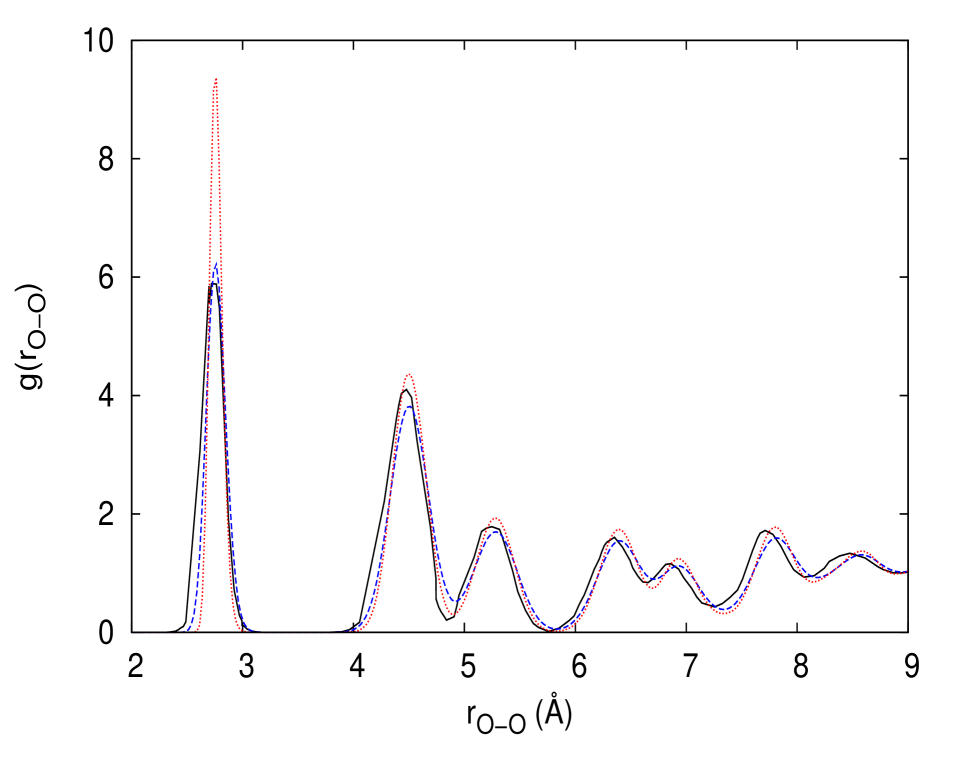
Figure 7: Radial distribution function of ice I_h for the TIP4PQ/2005 model using PIMC (dashed blue line) compared with the classical TIP4P/2005 model (dotted red line) and with experimental data (solid red line) Narten et al. (1976) at 77K and p=1 bar.

In Fig 5 the equation of state for ice I_h is plotted. The TIP4PQ/2005 state points are equidistant from those of TIP4P/2005_(PI), but they are now much closer to the experimental values, with a deviation of around 0.005 g/cm³, which amounts to a difference of only 0.8% with respect to the experimental value. Given the curvature of the equation of state, in line with the third law of thermodynamics, and the small difference between the TIP4PQ/2005 densities and the experimental results, leads us to believe that this is one of the best theoretical descriptions of ice I_h thus far seen in the literature. This is not to say that in the future this cannot be improved upon, for example via the inclusion of flexibility, polarisability etc. in the molecular model. In Fig. 7 the oxygen-oxygen radial distribution function of ice I_h at 77K is compared to the experimental results of Narten Narten et al. (1976), and the results are acceptable almost all the way up to 9Å. The most notable difference can be seen in the height of the first peak; which drops from 9.37 for classical TIP4P/2005, down to 6.21 for TIP4PQ/2005, compared to 5.95 experimentally Narten et al. (1976).

In an analogous study to that for 0K for TIP4P/2005_(PI) the relative stability of ices I_h, II, III, V and VI at low temperatures has been tabulated in Tables 5 and 8 and plotted in Fig. 8. As can be seen the relative energy between ice II and the remainder of the ices is similar to that of TIP4P/2005_(PI). The most significant result is that for TIP4PQ/2005 ice I_h regains its rightful place as the most stable ice phase. Experimentally the energy difference between I_h and II is 0.014 kcal/mol, which for TIP4PQ/2005 becomes 0.04 kcal/mol. In Table 9 results for the 0K coexistence pressures, calculated using equation 25, are presented. It can be seen that both the energies (Table 5) and the coexistence pressures (Table 9) for various transitions are substantially better than the values provided by classical simulations of the TIP4P/2005 model, in particular for the I_h-II transition. This gives us confidence that the TIP4PQ/2005 could well produce a respectable global phase diagram in the future.

IV Conclusions

This work addresses a series of physical properties of water that vary with the inclusion of atomic quantum delocalisation effects, which were introduced to the TIP4P/2005 model using path integral Monte Carlo simulations. Quantum simulations have been undertaken for all of the ice phases of water, with the exception of ice X, for the TIP4P/2005 model, and for the new TIP4PQ/2005 model. Using the Müser and Berne propagator for rigid asymmetric tops, various properties of these ices have been examined.

It has been found that the radial distribution functions become more ‘washed-out’ when quantum effects are taken into account. In other words, the peaks become lower and wider and shift to slightly larger distances. This goes hand-in-hand with a reduction in density for the quantum solid; by $\approx 0.02$ g/cm³ for temperatures above 150K, and $\approx$ 0.04 g/cm³ below 100K.

If a classical empirical model is tailored to reproduce the experimental ice densities at a temperature close to the melting point, as the temperature is reduced the model will start to fail (such is the case, for example, of the TIP4P/2005 model Noya et al. (2007)). This is due to the fact that classical simulations are unable to satisfy one of the consequences of the third law of thermodynamics, namely that the coefficient of thermal expansion, $\alpha$, tends to zero as the temperatures approaches zero Kelvin. It can be seen that the PIMC simulations now, to a good degree, correctly describe the low temperature physics of this model.

The translational component of the kinetic energy bears a passing resemblance to the classical value of $(3/2)RT$, whereas the rotational component is markedly larger.

There is a particularly pronounced effect in the relative stabilities of ices I_h and II, where the stability of ice II is enhanced by the inclusion of atomic quantum delocalisation effects.

In this work a re-parameterisation of the TIP4P/2005 model is provided that ‘compensates’ for the quantum effects so as to maintain the quantitative performance of the TIP4P/2005 model, whilst at the same time reproducing the correct physics at low temperatures. In this new model, which we have called TIP4PQ/2005, the only parameter to have changed is that of the dipole moment; the charge on the hydrogen atom has been increased by 0.02$e$, thus the dipole moment increases from 2.30D to 2.38D.

In this paper it is shown that the TIP4PQ/2005 model provides a good description of the densities of the ice phases for the state points considered. The ice I_h $p=1$ bar isobar has been calculated and the tendency for $\alpha$ to become zero is now present in the equation of state. This new model also correctly describes the relative stabilities of ices I_h and II. An extrapolation indicates that at 0K I_h is more stable than ice II by 0.04 kcal/mol (compared to 0.014 kcal/mol experimentally). The inclusion of quantum effects substantially improves the overall description of all of the ice phases studied here. The TIP4P/2005 does a reasonable job, but the TIP4PQ/2005 is clearly superior. This paper can be regarded as a first step in introducing atomic quantum delocalisation effects in the description of the solid phases of water. However, it is by no means the last word, since obviously water is a flexible molecule. In our opinion the results in the present manuscript could be very useful as a point of departure for the development of a flexible model of water for use in path integral simulations, and provides valuable material from which to make comparisons. Such comparison would establish just how much of the quantum effects in water are due to intra and how much is due to the intermolecular degrees of freedom.

V Acknowledgements

The authors would like to thank J. L. Abascal for insightful conversations and M. I. J. Probert for his hospitality and illuminating discussions whilst one of the authors, C. V. was in York. We would also like to thank the reviewers for their useful comments regarding the manuscript. This work has been funded by grants FIS2007-66079-C02-01 and FIS2006-12117-C04-03 from the DGI (Spain), S-0505/ESP/0299 (MOSSNOHO) from the Comunidad Autonoma de Madrid, and 910570 from the Universidad Complutense de Madrid. E. G. N. would like to thank the MEC for a Juan de la Cierva fellowship.

Table 1: Parameters for both the TIP4P/2005 and the TIP4PQ/2005 models. The distance between the oxygen and hydrogen sites is $d_{\mathrm{OH}}$. The angle, in degrees, formed by hydrogen, oxygen, and the other hydrogen atom is denoted by $\angle$H-O-H. The Lennard-Jones site is located on the oxygen with parameters $\sigma$ and $\epsilon$. The charge on the proton is $q_{\mathrm{H}}$. The negative charge is placed in a point M at a distance $d_{\mathrm{OM}}$ from the oxygen along the H-O-H bisector.

Model	$d_{\mathrm{OH}}$ (Å)	$\angle$H-O-H	$\sigma$(Å)	$\epsilon/k_{B}$(K)	$q_{\mathrm{H}}$(e)	$d_{\mathrm{OM}}$(Å)
TIP4P/2005	0.9572	104.52	3.1589	93.2	0.5564	0.1546
TIP4PQ/2005	0.9572	104.52	3.1589	93.2	0.5764	0.1546

Table 2: Results for the TIP4P/2005_(PI) model for the systems studied, along with a comparison to classical results for the same model. All energies are in units of kcal/mol and the densities are in g$\cdot$cm^-3. The errors (in kcal/mol) are ${\mathcal{O}}(0.003)$ in $K_{\mathrm{translational}}$, ${\mathcal{O}}(0.02)$ in $K_{\mathrm{rotational}}$, ${\mathcal{O}}(0.02)$ in $U$, ${\mathcal{O}}(0.04)$ in $E$ and ${\mathcal{O}}(0.002)$ g$\cdot$cm^-3 in $\rho$ .

Phase (& No molecules)	$T$ (K)	$p$ (bars)	$(3/2)RT$	$K_{\mathrm{translational}}$	$K_{\mathrm{rotational}}$	$K_{\mathrm{total}}$	$U$	$E$	$U$ (classical)	$\rho$ (path-integral)	$\rho$ (classical)
Ih (432)	250	0	0.75	0.83	1.39	2.22	-12.38	-10.17	-13.35	0.899	0.920
Ic (216)	78	0	0.23	0.45	1.36	1.81	-13.03	-11.22	-14.58	0.906	0.943
II (432)	123	0	0.37	0.51	1.26	1.77	-12.83	-11.06	-14.07	1.160	1.198
III (324)	250	2800	0.75	0.83	1.35	2.18	-12.15	-9.96	-13.06	1.141	1.159
IV (432)	110	0	0.33	0.49	1.25	1.74	-12.44	-10.70	-13.74	1.248	1.292
V (504)	237.65	5300	0.71	0.80	1.35	2.14	-12.19	-10.04	-13.21	1.240	1.271
VI (360)	225	11000	0.67	0.78	1.34	2.12	-12.21	-10.10	-13.11	1.356	1.379
VII (432)	300	100000	0.89	1.05	1.44	2.49	-9.32	-6.83	-9.95	1.767	1.782
VIII (600)	77	24000	0.23	0.49	1.17	1.76	-11.31	-9.65	-12.50	1.573	1.616
IX (324)	165	2800	0.49	0.63	1.33	1.96	-12.80	-10.84	-13.95	1.160	1.190
XI (360)	77	0	0.23	0.45	1.36	1.81	-13.04	-11.23	-14.60	0.906	0.945
XII (540)	260	5000	0.77	0.86	1.34	2.20	-11.97	-9.77	-12.85	1.267	1.296
XIII (504)	80	1	0.24	0.44	1.25	1.69	-12.76	-11.07	-14.16	1.217	1.261
XIV (540)	80	1	0.24	0.44	1.27	1.71	-12.80	-11.09	-14.25	1.280	1.331

Table 3: Oxygen-oxygen radial distribution function of ice I_h for various water models at 250K and p=0 bar.

Model	peak 1		peak 2		Reference
	$r$	height	$r$	height
TIP4P (classical)	2.725Å	4.707	4.525Å	2.279	Vega et al. (2005)
TIP4P (path integral)	2.7625Å	4.167	4.5625Å	2.122	This work
TIP4P/2005 (classical)	2.7375Å	5.113	4.5125Å	2.382	This work
TIP4P/2005(PI)	2.7875Å	4.481	4.5875Å	2.270	This work
TIP4PQ/2005	2.7625Å	4.725	4.5375Å	2.405	This work

Table 4: Results for the TIP4P/2005_(PI) model for the low temperature ice phases at a pressure of 1 bar. The energies are in units of kcal/mol and the densities are in g$\cdot$cm^-3. The errors (in kcal/mol) are ${\mathcal{O}}(0.003)$ in $K_{\mathrm{translational}}$, ${\mathcal{O}}(0.02)$ in $K_{\mathrm{rotational}}$, ${\mathcal{O}}(0.02)$ in $U$, ${\mathcal{O}}(0.04)$ in $E$ and ${\mathcal{O}}(0.002)$ g$\cdot$cm^-3 in $\rho$ .

Phase	$T$ (K)	$K_{\mathrm{translational}}$	$K_{\mathrm{rotational}}$	$K_{\mathrm{total}}$	$U$	$E$	$\rho$
Ih	200	0.70	1.36	2.06	-12.62	-10.56	0.903
Ih	150	0.58	1.35	1.93	-12.84	-10.91	0.906
Ih	125	0.53	1.35	1.87	-12.92	-11.05	0.907
Ih	100	0.48	1.35	1.83	-12.99	-11.15	0.907
Ih	77	0.45	1.36	1.80	-13.02	-11.22	0.906
II	200	0.69	1.28	1.96	-12.54	-10.57	1.145
II	150	0.57	1.25	1.82	-12.77	-10.95	1.155
II	125	0.51	1.24	1.75	-12.85	-11.09	1.159
II	100	0.47	1.24	1.71	-12.92	-11.21	1.163
II	77	0.43	1.26	1.84	-12.94	-11.26	1.165
III	200	0.70	1.32	2.02	-12.35	-10.34	1.106
III	150	0.58	1.29	1.87	-12.58	-10.70	1.116
III	125	0.53	1.30	1.82	-12.66	-10.84	1.122
III	100	0.48	1.30	1.77	-12.74	-10.96	1.125
III	77	0.44	1.30	1.74	-12.77	-11.02	1.130
V	200	0.69	1.30	1.99	-12.28	-10.29	1.204
V	150	0.57	1.28	1.85	-12.51	-10.67	1.217
V	125	0.52	1.28	1.78	-12.60	-10.81	1.222
V	100	0.47	1.28	1.74	-12.67	-10.92	1.225
V	77	0.44	1.28	1.72	-12.70	-10.99	1.227
VI	200	0.69	1.27	1.96	-12.19	-10.22	1.282
VI	150	0.58	1.25	1.83	-12.41	-10.58	1.296
VI	125	0.51	1.25	1.76	-12.50	-10.74	1.302
VI	100	0.46	1.25	1.71	-12.57	-10.86	1.306
VI	77	0.43	1.26	1.69	-12.60	-10.91	1.309

Table 5: Comparison of the energies, $E$, at 0K for a selection of phases for both the TIP4P/2005_(PI) and the TIP4PQ/2005 models as well as results for the classical TIP4P/2005 model Aragones et al. (2007). The energies are in units of kcal/mol. The lowest energy (most stable phase) is shown in bold font. The lower section provides the relative energies with respect to ice II.

Ice	$E$ (0K estimate)
	TIP4P/2005	TIP4P/2005(PI)	TIP4PQ/2005	Experimental Whalley (1984)
Ih	-15.059	-11.240	-12.477	-11.315
II	-14.847	-11.290	-12.436	-11.301
III	-14.741	-11.048	-12.210	-11.100
V	-14.644	-11.013	-12.152	-11.088
VI	-14.513	-10.939	-12.033	-10.928
Ih	-0.212	0.050	-0.041	-0.014
II	0	0	0	0
III	0.106	0.242	0.226	0.201
V	0.203	0.277	0.285	0.213
VI	0.334	0.351	0.403	0.373

Table 6: PIMC results for the TIP4PQ/2005 model for the systems studied and their relation to the experimental densities. All energies are in units of kcal/mol and the densities are in g$\cdot$cm^-3. The errors (in kcal/mol) are ${\mathcal{O}}(0.003)$ in $K_{\mathrm{translational}}$, ${\mathcal{O}}(0.02)$ in $K_{\mathrm{rotational}}$, ${\mathcal{O}}(0.02)$ in $U$, ${\mathcal{O}}(0.04)$ in $E$ and ${\mathcal{O}}(0.002)$ g$\cdot$cm^-3 in $\rho$ .

Phase	$T$ (K)	$p$ (bars)	$(3/2)RT$	$K_{\mathrm{translational}}$	$K_{\mathrm{rotational}}$	$K_{\mathrm{total}}$	$U$	$E$	$\rho$ (path-integral)	$\rho$ (experimental)	Reference
Ih	250	0	0.75	0.83	1.45	2.28	-13.74	-11.46	0.921	0.920	Röttger et al. (1994)
Ic	78	0	0.23	0.46	1.43	1.89	-14.33	-12.44	0.925	0.931	Kuhs et al. (1987)
II	123	0	0.37	0.52	1.32	1.85	-14.06	-12.21	1.185	1.190	Fortes et al. (2005)
III	250	2800	0.75	0.84	1.41	2.25	-13.44	-11.18	1.159	1.165	Londono et al. (1993)
IV	110	0	0.33	0.50	1.32	1.82	-13.63	-11.81	1.276	1.272	Engelhardt and Kamb (1981)
V	237.65	5300	0.71	0.81	1.41	2.22	-13.43	-11.21	1.266	1.271	Gagnon et al. (1990)
VI	225	11000	0.67	0.79	1.39	2.18	-13.41	-11.23	1.377	1.373	Kuhs et al. (1984)
VII	300	100000	0.89	1.05	1.47	2.52	-10.37	-7.85	1.780	1.880	Hemley et al. (1987)
VIII	77	24000	0.23	0.50	1.23	1.73	-12.28	-10.56	1.592	1.628 (at 10K)	Kuhs et al. (1984)
IX	165	2800	0.49	0.64	1.39	2.04	-14.07	-12.03	1.182	1.194	Londono et al. (1993)
XI	77	0	0.23	0.46	1.43	1.89	-14.34	-12.46	0.926	0.934 (at 5K)	Line and Whitworth (1996)
XII	260	5000	0.77	0.87	1.40	2.27	-13.23	-10.96	1.297	1.292	Lobban et al. (1998)
XIII	80	1	0.24	0.46	1.32	1.77	-13.95	-12.17	1.242	1.244	Salzmann et al. (2006)
XIV	80	1	0.24	0.46	1.34	1.80	-13.99	-12.20	1.307	1.332	Salzmann et al. (2006)

Table 7: Unit cell parameters for the TIP4PQ/2005 model for a selection of ice phases. Experimental values are from Table 11.2 of Ref Petrenko and Whitworth, 1999. Note that for ice II the hexagonal unit cell, rather than the rhombohedral unit cell, is given. All distances are in angstroms.

Phase	$T$ (K)	$p$(bars)		unit cell
				experimental	simulation
Ih	250	0		a=4.518, c=7.356	a=4.483, c= 7.352
II	123	0		a=12.97, c=6.25	a= 12.98, c=6.23
III	250	2800		a=6.666, c=6.936	a=6.645, c=7.011
V	100	1		a=9.22, b =7.54,	a=9.06, b=7.64,
				c=10.35, $\beta=109.2^{\mathrm{o}}$	c=10.21, $\beta=108.6^{\mathrm{o}}$
VI	225	11000		a=6.181, c=5.698	a=6.167, c=5.713

Table 8: PIMC results for the TIP4PQ/2005 model for the low temperature ice phases at a pressure of 1 bar. All energies are in units of kcal/mol and the densities are in g$\cdot$cm^-3. The errors (in kcal/mol) are ${\mathcal{O}}(0.003)$ in $K_{\mathrm{translational}}$, ${\mathcal{O}}(0.02)$ in $K_{\mathrm{rotational}}$, ${\mathcal{O}}(0.02)$ in $U$, ${\mathcal{O}}(0.04)$ in $E$ and ${\mathcal{O}}(0.002)$ g$\cdot$cm^-3 in $\rho$ .

Phase	$T$ (K)	$K_{\mathrm{translational}}$	$K_{\mathrm{rotational}}$	$K_{\mathrm{total}}$	$U$	$E$	$\rho$
Ih	300	0.97	1.49	2.47	-13.46	-10.99	0.915
Ih	200	0.71	1.44	2.15	-13.98	-11.82	0.925
Ih	150	0.60	1.42	2.02	-14.18	-12.16	0.928
Ih	125	0.54	1.41	1.96	-14.25	-12.29	0.928
Ih	100	0.50	1.42	1.92	-14.32	-12.40	0.928
Ih	77	0.46	1.43	1.89	-14.34	-12.45	0.927
II	125	0.53	1.32	1.84	-14.06	-12.21	1.185
II	100	0.48	1.30	1.78	-14.14	-12.35	1.188
II	77	0.44	1.32	1.76	-14.16	-12.40	1.190
III	150	0.59	1.36	1.95	-13.83	-11.88	1.134
III	125	0.54	1.36	1.90	-13.92	-12.02	1.139
III	100	0.50	1.37	1.87	-13.98	-12.12	1.142
III	77	0.45	1.37	1.82	-14.01	-12.19	1.146
V	125	0.53	1.34	1.84	-13.80	-11.93	1.248
V	100	0.49	1.34	1.82	-13.88	-12.06	1.251
V	77	0.44	1.35	1.79	-13.91	-12.12	1.253
VI	125	0.53	1.32	1.85	-13.67	-11.82	1.330
VI	100	0.48	1.31	1.79	-13.74	-11.95	1.334
VI	77	0.45	1.32	1.77	-13.77	-12.00	1.336

Table 9: Estimates of the coexistence pressures (in bar) for the TIP4PQ/2005 model extrapolated to 0K. Experimental values are taken from the work of Whalley Whalley (1984) and the values for the classical TIP4P/2005 model are from Aragones et al. (2007).

Phases	TIP4P/2005	TIP4PQ/2005	Experimental value
Ih-II	2090	400	$140\pm 200$
Ih-III	3630	3008	$2400\pm 100$
II-V	11230	15630	$18500\pm 4000$
II-VI	8530	10190	$10500\pm 1000$
III-V	3060	1800	$3000\pm 100$
V-VI	6210	5580	$6200\pm 200$

Figure 1: Kinetic rotational energy from PIMC simulations of the isolated H₂O molecule (filled circles) as a function of temperature. Between 10 and 50 replicas (P) have been used, depending on the temperature. There is good agreement between the simulation data and the rotational energy obtained from the theoretical partition function of an asymmetric top having the H₂O geometry (solid line). The magnitude of the error is less than the size of the symbols shown.

Figure 6: Plot of the total energy of ices I_h, II, III, V and VI at low temperatures for p=1 bar for TIP4P/2005_(PI). Lines correspond to the fit $E=a+bT^{4}$. The error in the total energy is of order $\pm 0.04$ kcal/mol.

Figure 8: Plot of the total energy of ices I_h, II, III, V and VI at low temperatures for p=1 bar for the TIP4PQ/2005 model. Lines correspond to the fit $E=a+bT^{4}$. The error in the total energy is of order $\pm 0.04$ kcal/mol.

References

- Eisenberg and Kauzmann (1969) D. Eisenberg and W. Kauzmann, The Structure and Properties of Water (Oxford University Press, 1969).
- Petrenko and Whitworth (1999) V. F. Petrenko and R. W. Whitworth, Physics of Ice (Oxford University Press, 1999).
- Franks (2000) F. Franks, Water: A Matrix of Life (RSC Publishing, 2000), 2nd ed.
- Ball (2001) P. Ball, Life’s Matrix: A Biography of Water (University of California Press, 2001).
- boo (2009) Water - From Interfaces to the Bulk, Faraday Discussions No 141 (RSC Publishing, 2009).
- Sanz et al. (2004) E. Sanz, C. Vega, J. L. F. Abascal, and L. G. MacDowell, Phys. Rev. Lett. 92, 255701 (2004).
- Goncharov et al. (2005) A. F. Goncharov, N. Goldman, L. E. Fried, J. C. Crowhurst, I.-F. W. Kuo, C. J. Mundy, and J. M. Zaug, Phys. Rev. Lett. 94, 125508 (2005).
- Schwegler et al. (2008) E. Schwegler, M. Sharma, F. Gygi, and G. Galli, Proc. Natl. Acad. Sci. USA 105, 14779 (2008).
- Benoit et al. (1998) M. Benoit, D. Marx, and M. Parrinello, Nature 392, 258 (1998).
- Loubeyre et al. (1999) P. Loubeyre, R. LeToullec, E. Wolanin, M. Hanfland, and D. Hausermann, Nature 397, 503 (1999).
- Liu et al. (2007) D. Liu, Y. Zhang, C.-C. Chen, C.-Y. Mou, P. H. Poole, and S.-H. Chen, Proc. Natl. Acad. Sci. USA 104, 9570 (2007).
- Xu et al. (2005) L. Xu, P. Kumar, S. V. Buldyrev, S.-H. Chen, P. H. Poole, F. Sciortino, and H. E. Stanley, Proc. Natl. Acad. Sci. USA 102, 16558 (2005).
- Kumar et al. (2007) P. Kumar, S. V. Buldyrev, S. R. Becker, P. H. Poole, F. W. Starr, and H. E. Stanley, Proc. Natl. Acad. Sci. USA 104, 9575 (2007).
- Poole et al. (1992) P. H. Poole, F. Sciortino, U. Essmann, and H. E. Stanley, Nature 360, 324 (1992).
- Debenedetti and Stanley (2003) P. G. Debenedetti and H. E. Stanley, Physics Today 56, 40 (2003).
- Debenedetti (2003) P. G. Debenedetti, J. Phys. Cond. Mat. 15, R1669 (2003).
- Stanley et al. (2000) H. E. Stanley, S. V. Buldyrev, M. Canpolat, O. Mishima, M. R. Sadr-Lahijany, A. Scala, and F. W. Starr, Phys. Chem. Chem. Phys. 2, 1551 (2000).
- Stanley et al. (1994) H. E. Stanley, C. A. Angell, U. Essmann, M. Hemmati, P. H. Poole, and F. Sciortino, Physica A 205, 122 (1994).
- Morrone and Car (2008) J. A. Morrone and R. Car, Phys. Rev. Lett. 101, 017801 (2008).
- Paesani and Voth (2009) F. Paesani and G. A. Voth, J. Phys. Chem. B 113, 5702 (2009).
- de la Peña and Kusalik (2006) L. H. de la Peña and P. G. Kusalik, J. Chem. Phys. 125, 054512 (2006).
- Miller and Manolopoulos (2005) T. F. Miller and D. E. Manolopoulos, J. Chem. Phys. 123, 154504 (2005).
- Gai et al. (1996) H. Gai, G. K. Schenter, and B. C. Garrett, J. Chem. Phys. 104, 680 (1996).
- de la Peña et al. (2005) L. H. de la Peña, M. S. G. Razul, and P. G. Kusalik, J. Chem. Phys. 123, 144506 (2005).
- Paesani and Voth (2008) F. Paesani and G. A. Voth, The Journal of Physical Chemistry C 112, 324 (2008).
- Abascal and Vega (2005) J. L. F. Abascal and C. Vega, J. Chem. Phys. 123, 234505 (2005).
- Vega et al. (2009) C. Vega, J. L. F. Abascal, M. M. Conde, and J. L. Aragones, Faraday Discussions 141, 251 (2009).
- Jorgensen et al. (1983) W. L. Jorgensen, J. Chandrasekhar, J. D. Madura, R. W. Impey, and M. L. Klein, J. Chem. Phys. 79, 926 (1983).
- Mahoney and Jorgensen (2000) M. W. Mahoney and W. L. Jorgensen, J. Chem. Phys. 112, 8910 (2000).
- Berendsen et al. (1987) H. J. C. Berendsen, J. R. Grigera, and T. P. Straatsma, J. Phys. Chem. 91, 6269 (1987).
- Abascal et al. (2009) J. L. F. Abascal, E. Sanz, and C. Vega, Phys. Chem. Chem. Phys. 11, 556 (2009).
- Pi et al. (2009) H. L. Pi, J. L. Aragones, C. Vega, E. G. Noya, J. L. F. Abascal, M. A. Gonzalez, and C. McBride, Molec. Phys. 107, 365 (2009).
- Vega and de Miguel (2007) C. Vega and E. de Miguel, J. Chem. Phys. 126, 154707 (2007).
- Vega et al. (2006) C. Vega, J. L. F. Abascal, and I. Nezbeda, J. Chem. Phys. 125, 034503 (2006).
- Morse and Rice (1982) M. D. Morse and S. A. Rice, J. Chem. Phys. 76, 650 (1982).
- Whalley (1984) E. Whalley, J. Chem. Phys. 81, 4087 (1984).
- Feynman and Hibbs (1965) R. P. Feynman and A. R. Hibbs, Path-integrals and Quantum Mechanics (McGraw-Hill, 1965).
- Chandler and Wolynes (1981) D. Chandler and P. G. Wolynes, J. Chem. Phys. 74, 4078 (1981).
- Gillan (1990) M. J. Gillan, The path-integral simulation of quantum systems (Kluwer, The Netherlands, 1990), vol. 293 of NATO ASI Series C, chap. 6, pp. 155–188.
- Ceperley (1995) D. M. Ceperley, Rev. Modern Phys. 67, 279 (1995).
- Allen and Tildesley (1987) M. P. Allen and D. J. Tildesley, Computer Simulation of Liquids (Oxford University Press, Oxford, 1987), chap. 10.
- Markland and Manolopoulos (2008) T. E. Markland and D. E. Manolopoulos, J. Chem. Phys. 129, 024105 (2008).
- Poulsen et al. (2005) J. A. Poulsen, G. Nyman, and P. J. Rossky, Proc. Natl. Acad. Sci. USA 102, 6709 (2005).
- Habershon et al. (2008) S. Habershon, G. S. Fanourgakis, and D. E. Manolopoulos, J. Chem. Phys. 129, 074501 (2008).
- Powles and Rickayzen (1979) J. G. Powles and G. Rickayzen, Molec. Phys. 38, 1875 (1979).
- Dong and Li (200) S. Dong and J. Li, Physica B 276-278, 469 (2000).
- Marx and Müser (1999) D. Marx and M. H. Müser, J. Phys. Cond. Mat. 11, R117 (1999).
- Müser and Berne (1996) M. H. Müser and B. J. Berne, Phys. Rev. Lett. 77, 2638 (1996).
- Zare (1988) R. N. Zare, Angular Momentum: Understanding spatial aspects in chamistry and physics (John Wiley & Sons Inc., 1988).
- Lobaugh and Voth (1997) J. Lobaugh and G. A. Voth, J. Chem. Phys. 106, 2400 (1997).
- Stern and Berne (2001) H. A. Stern and B. J. Berne, J. Chem. Phys. 115, 7622 (2001).
- Shinoda and Shiga (2005) W. Shinoda and M. Shiga, Phys. Rev. E 71, 041204 (2005).
- Mahoney and Jorgensen (2001) M. W. Mahoney and W. L. Jorgensen, J. Chem. Phys. 115, 10758 (2001).
- de Leeuw et al. (1980a) S. W. de Leeuw, J. W. Perram, and E. R. Smith, Proc. R. Soc. Lond. A 373, 27 (1980a).
- de Leeuw et al. (1980b) S. W. de Leeuw, J. W. Perram, and E. R. Smith, Proc. R. Soc. Lond. A 373, 57 (1980b).
- Bernal and Fowler (1933) J. D. Bernal and R. H. Fowler, J. Chem. Phys. 1, 515 (1933).
- Pauling (1935) L. Pauling, J. Am. Chem. Soc. 57, 2680 (1935).
- Buch et al. (1998) V. Buch, P. Sandler, and J. Sadlej, J. Phys. Chem. B 102, 8641 (1998).
- MacDowell et al. (2004) L. G. MacDowell, E. Sanz, C. Vega, and J. L. F. Abascal, J. Chem. Phys. 121, 10145 (2004).
- Barrat et al. (1989) J.-L. Barrat, P. Loubeyre, and M. L. Klein, J. Chem. Phys. 90, 5644 (1989).
- Müser et al. (1995) M. H. Müser, P. Nielaba, and K. Binder, Phys. Rev. B 51, 2723 (1995).
- Parrinello and Rahman (1980) M. Parrinello and A. Rahman, Phys. Rev. Lett. 45, 1196 (1980).
- Parrinello and Rahman (1982) M. Parrinello and A. Rahman, J. Chem. Phys. 76, 2662 (1982).
- Najafabadi and Yip (1983) R. Najafabadi and S. Yip, Scripta Metallurgica 17, 1199 (1983).
- Yashonath and Rao (1985) S. Yashonath and C. N. R. Rao, Molec. Phys. 54, 245 (1985).
- Levine (1975) I. N. Levine, Molecular Spectroscopy (John Wiley & Sons Inc., 1975).
- Ramirez and Herrero (2008) R. Ramirez and C. P. Herrero, J. Chem. Phys. 129, 204502 (2008).
- Vega et al. (2005) C. Vega, C. McBride, E. Sanz, and J. L. F. Abascal, Phys. Chem. Chem. Phys. 7, 1450 (2005).
- Kuharski and Rossky (1984) R. A. Kuharski and P. J. Rossky, Chem. Phys. Lett. 103, 357 (1984).
- Kuharski and Rossky (1985a) R. A. Kuharski and P. J. Rossky, J. Chem. Phys. 83, 5164 (1985a).
- Buono et al. (1991) G. S. D. Buono, P. J. Rossky, and J. Schnitker, J. Chem. Phys. 95, 3728 (1991).
- Kuharski and Rossky (1985b) R. A. Kuharski and P. J. Rossky, J. Chem. Phys. 83, 5289 (1985b).
- Soper (2000) A. K. Soper, Chem. Phys. 258, 121 (2000).
- Noya et al. (2007) E. G. Noya, C. Menduiña, J. L. Aragones, and C. Vega, The Journal of Physical Chemistry C 111, 15877 (2007).
- Feistel and Wagner (2006) R. Feistel and W. Wagner, J. Phys. Chem. Ref. Data 35, 1021 (2006).
- Tanaka (1998) H. Tanaka, J. Chem. Phys. 108, 4887 (1998).
- Koyama et al. (2004) Y. Koyama, H. Tanaka, G. Gao, and X. C. Zeng, J. Chem. Phys. 121, 7926 (2004).
- Aragones et al. (2007) J. L. Aragones, E. G. Noya, J. L. F. Abascal, and C. Vega, J. Chem. Phys. 127, 154518 (2007).
- (79) http://www.lsbu.ac.uk/water/.
- Paesani et al. (2006) F. Paesani, W. Zhang, D. A. Case, T. E. Cheatham III, and G. A. Voth, J. Chem. Phys. 125, 184507 (2006).
- Burnham and Xantheas (2002) C. J. Burnham and S. S. Xantheas, J. Chem. Phys. 116, 5115 (2002).
- Fanourgakis and Xantheas (2008) G. S. Fanourgakis and S. S. Xantheas, J. Chem. Phys. 128, 074506 (2008).
- Tironi et al. (1996) I. G. Tironi, R. M. Brunne, and W. F. van Gunsteren, Chem. Phys. Lett. 250, 19 (1996).
- Guillot (2002) B. Guillot, J. Molec. Liq. 101, 219 (2002).
- Röttger et al. (1994) K. Röttger, A. Endriss, J. Ihringer, S. Doyle, and W. F. Kuhs, Acta Crystallographica Section B Structural Science 50, 644 (1994).
- Kuhs et al. (1987) W. F. Kuhs, D. V. Bliss, and J. L. Finney, J. de Physique Colloques 48, C1 (1987).
- Fortes et al. (2005) A. D. Fortes, I. G. Wood, M. Alfredsson, L. Vocadlo, and K. S. Knight, J. App. Crystallography 38, 612 (2005).
- Londono et al. (1993) J. D. Londono, W. F. Kuhs, and J. L. Finney, J. Chem. Phys. 98, 4878 (1993).
- Engelhardt and Kamb (1981) H. Engelhardt and B. Kamb, J. Chem. Phys. 75, 5887 (1981).
- Gagnon et al. (1990) R. E. Gagnon, H. Kiefte, M. J. Clouter, and E. Whalley, J. Chem. Phys. 92, 1909 (1990).
- Kuhs et al. (1984) W. F. Kuhs, J. L. Finney, C. Vettier, and D. V. Bliss, J. Chem. Phys. 81, 3612 (1984).
- Hemley et al. (1987) R. J. Hemley, A. P. Jephcoat, H. K. Mao, C. S. Zha, L. W. Finger, and D. E. Cox, Nature 330, 737 (1987).
- Line and Whitworth (1996) C. M. B. Line and R. W. Whitworth, J. Chem. Phys. 104, 10008 (1996).
- Lobban et al. (1998) C. Lobban, J. L. Finney, and W. F. Kuhs, Nature 391, 268 (1998).
- Salzmann et al. (2006) C. G. Salzmann, P. G. Radaelli, A. Hallbrucker, E. Mayer, and J. L. Finney, Science 311, 1758 (2006).
- Narten et al. (1976) A. H. Narten, C. G. Venkatesh, and S. A. Rice, J. Chem. Phys. 64, 1106 (1976).