Quantum gravity as sum over spacetimes

1 Introduction

A major unsolved problem in theoretical physics is to reconcile the classical theory of general relativity with quantum mechanics. These lectures will deal with an attempt to describe quantum gravity as a path integral over geometries. Such an approach has to be non-perturbative since gravity is a non-renormalizable quantum field theory when the dimension of spacetime is four. In that case the dimension of the gravitational coupling constant $G$ is -2 in units where $\hbar=1$ and $c=1$ and the dimension of mass is one. Thus conventional, perturbative quantum field theory is only expected to be good for energies

$$E^{2}\ll 1/{G}.$$ (1)

That is still perfectly good in all experimental situations we can imagine in the laboratory, but an indication that something “new” has to happen at sufficiently large energy, or equivalently, at sufficiently short distances. It is possible, or maybe even likely, that a breakdown of perturbation theory when (1) is not satisfied indicates that new degrees of freedom should be present in a theory valid at higher energies. Indeed, we have a well known example in the electroweak theory. Originally the electroweak theory was described by a four-fermion interaction. Such a theory is not renormalizable and perturbation theory breaks down at sufficiently high energy. In fact it breaks down unless the energy satisfies (1) with the gravitational coupling constant $G$ replaced the coupling constant $G_{F}$ in front of the four-Fermi interaction (since $G_{F}$ also has mass dimension -2). The breakdown reflects the appearance of new degrees of freedom, the $W$ and the $Z$ particles, and the four-Fermi interaction is now just an approximation to the process where a fermion interacts via $W$ and $Z$ particles with another fermion. The corresponding electroweak theory is renormalizable.

When it comes to gravity there seems to be no “simple” fix like the one just described. However, string theory is an example of a theory which tries to solve the problem by adding (infinitely many) new degrees of freedom. Loop quantum gravity is another approach to quantum gravity which tries to circumvent the problem of non-renormalizability by introducing rules of quantization which are unconventional from a perturbative point of view. The point of view taken here in these lectures is much more mundane. In a sum-over-histories approach we will attempt to define a non-perturbative quantum field theory which has as its infrared limit ordinary classical general relativity and at the same time has a nontrivial ultraviolet limit. From this point of view it is in the spirit of the renormalization group approach, first advocated long ago by Weinberg weinberg , and more recently substantiated by several groups of researchers reuteretc .

To understand the possibility of a nontrivial ultraviolet fixed point let us first apply ordinary perturbation theory to quantum gravity in a regime where (1) is satisfied. One can in a reliable way calculate the lowest-order quantum correction to the gravitational potential of a point particle:

$$\frac{G}{r}\to\frac{G(r)}{r},~{}~{}~{}G(r)=G\left(1-\omega\frac{G}{r^{2}}+\cdots\right),~{}~{}~{}\omega=\frac{167}{30\pi}.$$ (2)

Thus the gravitational coupling constant becomes scale-dependent and transferring from distance to energy we have

$$G(E)=G(1-\omega GE^{2}+\cdots)\approx\frac{G}{1+\omega GE^{2}}.$$ (3)

It should be stressed that the scenario described in (2) and (3) is completely standard in quantum field theory. Let us take the simplest quantum field theory relevant in nature: quantum electrodynamics. The electron as we observe it in low-energy scattering experiments is screened by vacuum polarization: virtual electron-positron pairs, created out of the vacuum and annihilated again so fast that one has consistency with the energy-time uncertainty relations, act like dipoles and the observed charge becomes less than the “bare” charge. To lowest order (one loop) (2) and (3) are replaced by

$$\frac{e^{2}}{r}\to\frac{e^{2}(r)}{r},~{}~{}~{}e(r)=e\left(1-\frac{e^{2}}{6\pi^{2}}\ln(m\,r)\right)+\cdots),~{}~{}~{}m\,r\ll 1.$$ (4)

$$e^{2}(E)=e^{2}\left(1+\frac{e^{2}}{6\pi^{2}}\ln(E/m)\right)+\cdots)\approx\frac{e^{2}}{1-\frac{e^{2}}{6\pi^{2}}\ln(E/m)}.$$ (5)

The last expression in eq. (5) is precisely the renormalization group-improved formula for the running coupling constant in QED. In fact, it is easy to calculate the so-called (one-loop) $\beta$-function for QED from the first equation in (5) and use this $\beta$-function to obtain the expression on the left-hand side of (5). Contrary to (3) it breaks down for sufficiently high energy: it has a so-called Landau pole and it reflects that we expect the interactions of QED to be infinitely strong at short distances. We do not believe that such quantum field theories really exist as “stand-alone” theories. They either require an explicit cut-off, which will then enter in the observables at high energies, or they have to be embedded in a larger theory without a Landau pole.

Assume that the last expression in (3) was exact for all $E$ (which it is not). One can argue that one should use $G(E)$ in eq. (1) rather than $G$, in which case one obtains

$$G(E)E^{2}<\frac{1}{\omega}=\frac{30\pi}{167}~{}~{}~{}(<1).$$ (6)

Thus, assuming (3) it suddenly seems as if quantum gravity had become a reliable quantum theory at all energy scales, the reason being that the effective coupling constant $G(E)$ becomes weaker at high energies. The behaviour (3) can be described in terms of a $\beta$-function for quantum gravity. Introduce the dimensionless coupling constant ${\tilde{G}}(E)$:

$${\tilde{G}}(E)=G(E)E^{2}.$$ (7)

From (3) it follows that ${\tilde{G}}(E)$ satisfies the following equation:

$$E\frac{\mbox{d}{\tilde{G}}}{\mbox{d}E}=\beta({\tilde{G}}),~{}~{}~{}~{}\beta({\tilde{G}})=2{\tilde{G}}-2\omega{\tilde{G}}^{2}.$$ (8)

The zeros of $\beta({\tilde{G}})$ determine the fixed points of the running coupling constant ${\tilde{G}}(E)$. The zero at ${\tilde{G}}=0$ is an infrared fixed point: for $E\to 0$ the coupling constant ${\tilde{G}}(E)\to 0$ and correspondingly the coupling constant $G(E)\to G$. The zero at ${\tilde{G}}=1/\omega$ is an ultraviolet fixed point : for $E\to\infty$ the coupling constant ${\tilde{G}}(E)\to 1/\omega$ (and $G(E)\to 0$ as $1/(\omega E^{2})$).

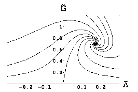
Figure 1: The flow of dimensionless gravitational and cosmological coupling constants ${\tilde{G}}$ and ${\tilde{\Lambda}}$ from a UV fixed point. One line flows to the infrared Gaussian fixed point where ${\tilde{G}}$ and ${\tilde{\Lambda}}$ are zero.

While there is no compelling reason to take the above arguments very seriously, since they are based on a one-loop calculation, the claim in reuteretc is that a more careful analysis using the so-called exact renormalization group equations or a systematic $2+\varepsilon$ expansion confirms the picture of a non-trivial UV fixed point. A typical result of the renormalization group calculation is shown in Fig. 1 in the case where the effective action has been “truncated” to just include the Einstein term and a cosmological term. The figure has a UV fixed point from where the flow to low energies starts and an infrared fixed point (the origin in the coupling constant coordinate system).

Where do we meet such scenarios (IR fixed points at zero coupling and a nontrivial UV fixed point for a suitably defined dimensionless coupling constant)? Assume one has an asymptotically free field theory in $d$ dimensions, i.e. $g=0$ is an UV fixed point. The strong interactions in four-dimensional flat spacetime, quantum chromodynamics (QCD), are such a theory. In high-energy scattering experiments the effective, running coupling constant goes to zero. This has been beautifully verified in high-energy experiments. The non-linear sigma model in two-dimensional spacetime is another model. It plays a very important role in string theory, but even before that was extensively studied as a toy model of QCD since it is asymptotically free (i.e. the running, effective coupling constant goes to zero at high energies). The asymptotically free theories have a negative $\beta$-function. This is what makes the running coupling constant go to zero at high energies. Change now (artificially) the dimension of spacetime infinitesimally from $d$ to $d+\varepsilon$. Then the $\beta$-function to lowest order in $\varepsilon$ will change as follows:

$$\beta_{d}(g)\to\beta_{d+\varepsilon}=\varepsilon g+\beta_{g}(g),$$ (9)

and the situation is as shown in Fig. 2: $g=0$ changes from an UV fixed point to an infrared fixed point while the new UV fixed point will be displaced to finite positive value $g_{c}(\varepsilon)$ of $g$, a value which goes to zero when $\varepsilon$ goes to zero. In the case of gravity we have formally a renormalizable theory when $d=2$, the dimension where the gravitational coupling constant $G$ is dimensionless. One can show that the two-dimensional theory can be viewed as asymptotically free (see eq. (113) below) To apply eq. (9) to four-dimensional quantum gravity starting with a renormalizable theory of gravity means that $\varepsilon$ has to be two, which is not very small. Thus the considerations above make little sense at a quantitative level, but the use of the exact renormalization group indicates, as mentioned, that the qualitative picture is correct.

\psfrag{B}{{\bf{\LARGE$\beta(g)$}}}\includegraphics{beta-f.eps}

Figure 2: The change in the beta function $\beta(g)$ in an asymptotically free theory when the dimension changes from the critical dimension $d$, where the coupling constant $g$ is dimensionless, to $d+\varepsilon$.

The discussion above shows that there might be a chance that quantum gravity can be defined as an ordinary quantum field theory at a non-trivial ultraviolet fixed point. It clearly requires non-perturbative tools to address the question of the existence of such a fixed point and to analyze the properties of the field theory defined by approaching the fixed point. One way to proceed is by using a lattice regularization of the quantum field theory in question. The lattice provides an UV regularization of the quantum field theory, namely, the inverse lattice spacing $1/a$. The task is then to define a suitable “continuum” limit of this lattice theory. The procedure used is typically as follows: let ${\cal O}(x_{n})$ be an observable, $x_{n}$ denoting a lattice point. We write $x_{n}=a\,n$, $n$ measuring the position in integer lattice spacings. One can then obtain, either by computer simulations or by analytical calculations, the correlation length $\xi(g_{0})$ in lattice units, from

$$-\log\langle{\cal O}(x_{n}){\cal O}(y_{m})\rangle\sim|n-m|/\xi(g_{0})+o(|n-m|).$$ (10)

A continuum limit of the lattice theory may then exist if it is possible to fine-tune the bare coupling constant $g_{0}$ of the theory to a critical value $g_{0}^{c}$ such that the correlation length goes to infinity, $\xi(g_{0})\to\infty$. Knowing how $\xi(g_{0})$ diverges for $g_{0}\to g_{0}^{c}$ determines how the lattice spacing $a$ should be taken to zero as a function of the coupling constants, namely,

$$\xi(g_{0})\propto\frac{1}{|g_{0}-g_{0}^{c}|^{\nu}},~{}~{}~{}~{}~{}a(g_{0})\propto|g_{0}-g_{0}^{c}|^{\nu}.$$ (11)

This particular scaling of the lattice spacing ensures that one can define a physical mass $m_{ph}$ by

$$m_{ph}a(g_{0})=1/\xi(g_{0})$$

such that the correlator $\langle{\cal O}(x_{n}){\cal O}(y_{m})\rangle$ falls off exponentially like $\mbox{e}^{-m_{ph}|x_{n}-y_{m}|}$ for $g_{0}\to g_{0}^{c}$ when $|x_{n}-y_{m}|$, but not $|n-m|$, is kept fixed in the limit $g_{0}\to g_{0}^{c}$. Thus we have created a picture where the underlying lattice spacing goes to zero while the physical mass (or the correlation length measured in physical length units, not in lattice spacings) is kept fixed. This is the standard Wilsonian scenario for obtaining the continuum (Euclidean) quantum field theory associated with the critical point $g_{0}^{c}$ of a second order phase transition (for second-order phase transitions there exists a correlation length which diverges, usually associated with the order parameter characterizing the transition).

We would like to apply a similar approach to quantum gravity, and thus obtain a new way to investigate if quantum gravity can be defined non-perturbatively as a quantum field theory. The predictions from such a theory could then be compared with the renormalization group predictions related to the asymptotic safety picture described above. It should be mentioned that the asymptotic safety picture is not the only suggestion for a continuum quantum theory of gravity using only “conventional” ideas of quantum field theory. Very recently two other scenarios have been suggested. One is called Lifshitz gravity horava and is a theory where the non-renormalizability of the Einstein-Hilbert theory is cured by adding higher-order spatial derivatives in a way somewhat similar to what Lifshitz did many years ago in statistical models. In fact, the setup of the theory has some resemblance with the lattice-theory setup of “Causal Dynamical Triangulations (CDT)” , to be described below, since a time foliation is assumed and the infrared limit is that of GR. However, contrary to Lifshitz gravity, we do not attempt to put in higher spatial derivatives in the lattice theory. However, when a continuum limit in the lattice theory is taken in a specific way which is not entirely symmetric in space and time one cannot rule out that higher spatial derivatives can play a role. The other model goes by the name of “scale-invariant gravity” shaposh1 ; shaposh2 . It modifies gravity into a renormalizable theory by introducing a scalar degree of freedom in addition to the transverse gravitational degrees of freedom. Also this model has interesting features not incompatible with the results of computer simulations using the CDT lattice model.

As already mentioned, we will use a lattice approach known as causal dynamical triangulations (CDT) as a regularization. In Sec. 2 we give a short description of the formalism, providing the definitions which are needed later to describe the measurements. CDT establishes a non-perturbative way of performing the sum over four-geometries (for more extensive definitions, see ajl4d ; blp ). It sums over the class of piecewise linear four-geometries which can be assembled from four-dimensional simplicial building blocks of link length $a$, such that only causal spacetime histories are included. The challenge when searching for a field theory of quantum gravity is to find a theory which behaves as described above, i.e. as in eq. (11). The challenge is three-fold: (i) to find a suitable non-perturbative formulation of such a theory which satisfies a minimum of reasonable requirements, (ii) to find observables which can be used to test relations like (10), and (iii) to show that one can adjust the coupling constants of the theory such that (11) is satisfied. Although we will focus on (i) in what follows, let us immediately mention that (ii) is notoriously difficult in a theory of quantum gravity, where one is faced with a number of questions originating in the dynamical nature of geometry. What is the meaning of distance when integrating over all geometries? How do we attach a meaning to local spacetime points like $x_{n}$ and $y_{n}$? How can we define at all local, diffeomorphism-invariant quantities in the continuum which can then be translated to the regularized (lattice) theory? – What we want to point out here is that although (i)-(iii) are standard requirements when relating critical phenomena and (Euclidean) quantum field theory, gravity is special and may require a reformulation of (part of) the standard scenario sketched above. We will return to this issue later.

Our proposed non-perturbative formulation of four-dimensional quantum gravity has a number of nice properties.

First, it sums over a class of piecewise linear geometries. The characteristic feature of piecewise linear geometries is that they admit a description without the use of coordinate systems. In this way we perform the sum over geometries directly, avoiding the cumbersome procedure of first introducing a coordinate system and then getting rid of the ensuing gauge redundancy, as one has to do in a continuum calculation. Our underlying assumptions are that 1) the class of piecewise linear geometries is in a suitable sense dense in the set of all geometries relevant for the path integral (probably a fairly mild assumption), and 2) that we are using a correct measure on the set of geometries. This is a more questionable assumption since we do not even know whether such a measure exists. Here one has to take a pragmatic attitude in order to make progress. We will simply examine the outcome of our construction and try to judge whether it is promising.

Secondly, our scheme is background-independent. No distinguished geometry, accompanied by quantum fluctuations, is put in by hand. If the CDT-regularized theory is to be taken seriously as a potential theory of quantum gravity, there has to be a region in the space spanned by the bare coupling constants where the geometry of spacetime bears some resemblance with the kind of universe we observe around us. That is, the theory should create dynamically an effective background geometry around which there are (small) quantum fluctuations. This is a very nontrivial property of the theory and one we are going to investigate in some detail. Computer simulations presented in these lectures confirm in a much more direct way the indirect evidence for such a scenario which we have known for some time and first reported in emerge ; semi . They establish the de Sitter nature of the background spacetime, quantify the fluctuations around it, and set a physical scale for the universes we are dealing with. The main results of these investigations, without the numerical details, were announced in agjl and a detailed account of the results was presented in bigs4 .

The remainder of these lecture notes is organized as follows: in Sec. 2 we describe the lattice formulation of four-dimensional quantum gravity. In Sec. 3 the numerical results in 4d are summarized. We view these results as very important, but they also serve as a motivation for moving to two dimensions. While there is no propagating graviton in two-dimensional quantum gravity, it is a diffeomorphism-invariant theory and almost all of the conceptional problems mentioned above are present there. Thus it is an important exercise to solve two-dimensional quantum gravity. Surprisingly this can be done in the lattice regularization known as “dynamical triangulation”. An important corollary is that (1) one can explicitly construct the continuum limit of the lattice theory and (2) show that it agrees with the so-called Liouville 2d quantum gravity theory. This latter theory is a continuum conformal field theory, explicit solvable, and, when viewed in the correct way, a diffeomorphism-invariant theory. Thus there is indeed no problem having a lattice regularization of a diffeomorphism-invariant theory. In Sec. 4 we solve what is known as two-dimensional Euclidean quantum gravity. In Sec. 5 we show how one can interpolate from Euclidean 2d quantum gravity to “Lorentzian” 2d quantum gravity which is a two-dimensional version of the four-dimensional gravity theory we have discussed in Sec. 3. Finally Sec. 7 discusses the results obtained and outlines perspectives.

2 CDT

The use of so-called causal dynamical triangulations (CDT) stands in the tradition of teitelboim , which advocated that in a gravitational path integral with the correct, Lorentzian signature of spacetime one should sum over causal geometries only. More specifically, we adopted this idea when it became clear that attempts to formulate a Euclidean non-perturbative quantum gravity theory run into trouble in spacetime dimension $d$ larger than two as will be described below.

This implies that we start from Lorentzian simplicial spacetimes with $d=4$ and insist that only causally well-behaved geometries appear in the (regularized) Lorentzian path integral. A crucial property of our explicit construction is that each of the configurations allows for a rotation to Euclidean signature. We rotate to a Euclidean regime in order to perform the sum over geometries (and rotate back again afterward if needed). We stress here that although the sum is performed over geometries with Euclidean signature, it is different from what one would obtain in a theory of quantum gravity based ab initio on Euclidean spacetimes. The reason is that not all Euclidean geometries with a given topology are included in the “causal” sum since in general they have no correspondence to a causal Lorentzian geometry.

\psfrag{a}{{\bf{\LARGE$t_{i}$}}}\psfrag{b}{{\bf{\LARGE$t_{f}$}}}\psfrag{c}{{\bf{\LARGE$x_{i}$}}}\psfrag{d}{{\bf{\LARGE$x_{f}$}}}\psfrag{t}{{\bf{\LARGE$t$}}}\psfrag{x}{{\bf{\LARGE$x$}}}\psfrag{u}{{\bf{\LARGE$a$}}}\includegraphics{line.eps}

\psfrag{a}{{\bf{\LARGE$t_{i}$}}}\psfrag{b}{{\bf{\LARGE$t_{f}$}}}\psfrag{c}{{\bf{\LARGE$x_{i}$}}}\psfrag{d}{{\bf{\LARGE$x_{f}$}}}\psfrag{t}{{\bf{\LARGE$t$}}}\psfrag{x}{{\bf{\LARGE$x$}}}\psfrag{u}{{\bf{\LARGE$a$}}}\includegraphics{line3d_a.ps}

Figure 3: Piecewise linear space-time histories in quantum mechanics and in (1+1)-dimensional quantum gravity. In the gravity case we show only a single space-time history, while in the quantum particle case we show many such histories as well as the average path (thick line).

We refer to ajl4d for a detailed description of how to construct the class of piecewise linear geometries used in the Lorentzian path integral. The most important assumption is the existence of a global proper-time foliation. This is symbolically illustrated in Fig. 3 where we compare the construction to the one of ordinary quantum mechanics: the path integral of ordinary quantum mechanics is regularized as a sum over piecewise linear paths from point $x_{i}$ to point $x_{f}$ in time $t_{f}-t_{i}$. The time steps have length $a$ and the continuum limit is obtained when the length $a$ of these “building blocks” goes to zero. Similarly, in the quantum gravity case we have a sum over four-geometries, “stretching” between two three-geometries separated a proper time $t$ and constructed from four-dimensional building blocks, as described below. On the figure we show for illustrational simplicity only a single space-time history and replace the three-dimensional spatial geometries with a one-dimensional one of $S^{1}$-topology. Moving from left to right we have a time foliation where at each discrete time step space is represented by a circle. Neighbouring circles are then connected by piecewise flat building blocks, usually triangles, as illustrated in Fig. 17 in Sec. 5. In the “real” four-dimensional case, the spatial slices of topology $S^{1}$ will be replaced by spatial slices of topology $S^{3}$, and neighbouring spatial $S^{3}$ slices are then connected by four-simplices as illustrated in Fig. 4 and described in detail below. There is an important difference between the quantum mechanical sum over paths and our sum over geometries with a time foliation: the time $t$ in the quantum mechanical example is an external parameter, while the time $t$ in the case of quantum gravity is intrinsic. Also, again for the purpose of illustration, the two-dimensional geometry has been drawn embedded in three-dimensional space, but in the path integral implementing the summation over geometries there is no such embedding present. Finally, we cannot refrain from mentioning that the paths shown for the quantum mechanical particle are in fact typical paths which appear for the (Euclideanized) path integral of a particle placed in an external potential. They are picked out from an actual Monte Carlo simulation of such a physical system. Similarly, the 2d surface is a surface picked out from a Monte Carlo simulation of 2d quantum gravity and thus corresponds to a typical 2d surface which appears in the path integral. This is the reason for the somewhat poor graphic representation: there is no natural length-preserving representation of the surface in 3d such that the surface is not self-intersecting. For better graphic illustrations (animations) of the 2d surfaces which appear in the 2d quantum-gravitational path integral we refer to the link link .

As mentioned above, we assume that the spacetime topology is that of $S^{3}\times R$, the spatial topology being that of $S^{3}$ merely for convenience. The spatial geometry at each discrete proper-time step $t_{n}$ is represented by a triangulation of $S^{3}$, made up of equilateral spatial tetrahedra with squared side-length $\ell_{s}^{2}\equiv a^{2}>0$. In general, the number $N_{3}(t_{n})$ of tetrahedra and how they are glued together to form a piecewise flat three-dimensional manifold will vary with each time-step $t_{n}$. In order to obtain a four-dimensional triangulation, the individual three-dimensional slices must still be connected in a causal way, preserving the $S^{3}$-topology at all intermediate times $t$ between $t_{n}$ and $t_{n+1}$ . This is done as illustrated in Fig. 4, introducing what we call (4,1)-simplices and (3,2)-simplices. More precisely, a $(4,1)$-simplex is a four-simplex with four of its vertices (i.e. a boundary tetrahedron) belonging to the triangulation of $S^{3}(t_{n})$, the time-slice corresponding to time $t_{n}$, and the fifth vertex belonging to the triangulation of $S^{3}(t_{n+1})$, the time-slice corresponding to time $t_{n+1}$. Similarly, a $(3,2)$ simplex has three vertices, i.e. a triangle, belonging to the triangulation of $S^{3}(t_{n})$ and two vertices, i.e. a link, belonging to the triangulation of $S^{3}(t_{n+1})$. We have also simplices of type $(1,4)$ and $(2,3)$, which are defined in an obvious way, interchanging the role of $S^{3}(t_{n})$ and $S^{3}(t_{n+1})$. One can show that two triangulations of $S^{3}(t_{n})$ and $S^{3}(t_{n+1})$ can be “connected” by these four building blocks glued together in a suitable way such that we have a four-dimensional triangulation of $S^{3}\times[0,1]$. Also, two given triangulations of $S^{3}(t_{n})$ and $S^{3}(t_{n+1})$ can be connected in many ways compatible with the topology $S^{3}\times[0,1]$.

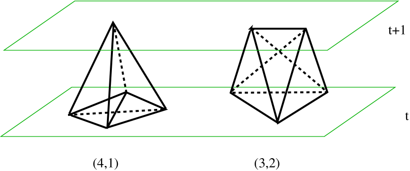
Figure 4: (4,1) and a (3,2) simplices connecting two neighbouring spatial slices. We also have symmetric (1,4) and (2,3) simplices with a vertex and a line, respectively, at time $t$ and a tetrahedron and a triangle, respectively, at time $t+1$. For simplicity we denote the total number of (4,1) and (1,4) simplices by $N^{(4,1)}_{4}$ and similarly the total number of (3,2) and (2,3) simplices by $N_{4}^{3,2}$.

In the path integral we will be summing over all possible ways to connect a given triangulation $S^{3}(t_{n})$ to a given triangulation of $S^{3}(t_{n+1})$ compatible with the topology $S^{3}\times[0,1]$. In addition we will sum over all 3d triangulations of $S^{3}$ at all times $t_{n}$.

We allow for an asymmetry between temporal and spatial lattice length assignments. Denote by $\ell_{t}$ and $\ell_{s}$ the length of the time-like links and the space-like links, respectively. Then $\ell_{t}^{2}\!=\!-\alpha\ell_{s}^{2}$, $\alpha>0$. The explicit rotation to Euclidean signature is done by performing the rotation $\alpha\to-\alpha$ in the complex lower half-plane, $|\alpha|>7/12$, such that we have $\ell_{t}^{2}=|\alpha|\ell_{s}^{2}$ (see ajl4d for a discussion).

The Einstein-Hilbert action $S^{\rm EH}$ has a natural geometric implementation on piecewise linear geometries in the form of the Regge action. This is given by the sum of the so-called deficit angles around the two-dimensional “hinges” (subsimplices in the form of triangles), each multiplied with the volume of the corresponding hinge. In view of the fact that we are dealing with piecewise linear, and not smooth metrics, there is no unique “approximation” to the usual Einstein-Hilbert action, and one could in principle work with a different form of the gravitational action. We will stick with the Regge action, which takes on a very simple form in our case, where the piecewise linear manifold is constructed from just two different types of building blocks. After rotation to Euclidean signature one obtains for the action (see blp for details)

$$S_{E}^{\rm EH} = \frac{1}{16\pi^{2}G}\int d^{4}x\sqrt{g}(-R+2\Lambda)~{}~{}\longrightarrow$$ (12)

$$S_{E}^{\rm Regge} = -(\kappa_{0}+6\Delta)N_{0}+\kappa_{4}(N_{4}^{(4,1)}+N_{4}^{(3,2)})+\Delta(2N_{4}^{(4,1)}+N_{4}^{(3,2)}),$$

where $N_{0}$ denotes the total number of vertices in the four-dimensional triangulation and $N_{4}^{(4,1)}$ and $N_{4}^{(3,2)}$ denote the total number of the four-simplices described above, so that the total number $N_{4}$ of four-simplices is $N_{4}=N_{4}^{(4,1)}+N_{4}^{(3,2)}$. The dimensionless coupling constants $\kappa_{0}$ and $\kappa_{4}$ are related to the bare gravitational and bare cosmological coupling constants, with appropriate powers of the lattice spacing $a$ already absorbed into $\kappa_{0}$ and $\kappa_{4}$. The asymmetry parameter $\Delta$ is related to the parameter $\alpha$ introduced above, which describes the relative scale between the (squared) lengths of space- and time-like links. It is both convenient and natural to keep track of this parameter in our set-up, which from the outset is not isotropic in time and space directions, see again blp for a detailed discussion. Since we will in the following work with the path integral after Wick rotation, let us redefine $\tilde{\alpha}:=-\alpha$ blp , which is positive in the Euclidean domain. For future reference, the Euclidean four-volume of our universe for a given choice of $\tilde{\alpha}$ is given by

$$V_{4}=\tilde{C}_{4}(\xi)\,a^{4}\,N_{4}^{(4,1)}=\tilde{C}_{4}(\xi)\,a^{4}\,N_{4}/(1+\xi),$$ (13)

where $\xi$ is the ratio

$$\xi=N_{4}^{(3,2)}/N_{4}^{(4,1)},$$ (14)

and $\tilde{C}_{4}(\xi)\,a^{4}$ is a measure of the “effective four-volume” of an “average” four-simplex. $\xi$ will depend on the choice of coupling constants in a rather complicated way (for a detailed discussion we refer to ajl4d ; bigs4 ).

The path integral or partition function for the CDT version of quantum gravity is now

$$Z(G,\Lambda)=\int{\cal D}[g]\;\mbox{e}^{-S_{E}^{\rm EH}[g]}~{}~{}~{}\to~{}~{}~{}Z(\kappa_{0},\kappa_{4},\Delta)=\sum_{{\cal T}}\frac{1}{C_{\cal T}}\;\mbox{e}^{-S_{E}({\cal T})},$$ (15)

where the summation is over all causal triangulations ${\cal T}$ of the kind described above, and we have dropped the superscript “Regge” on the discretized action. The factor $1/C_{\cal T}$ is a symmetry factor, given by the order of the automorphism group of the triangulation ${\cal T}$. The actual set-up for the simulations is as follows. We choose a fixed number $N$ of spatial slices at proper times $t_{1}$, $t_{2}=t_{1}+a_{t}$, up to $t_{N}=t_{1}+(N\!-\!1)a_{t}$, where $\Delta t\equiv a_{t}$ is the discrete lattice spacing in temporal direction and $T=Na_{t}$ the total extension of the universe in proper time. For convenience we identify $t_{N+1}$ with $t_{1}$, in this way imposing the topology $S^{1}\times S^{3}$ rather than $I\times S^{3}$. This choice does not affect physical results, as will become clear in due course.

Our next task is to evaluate the non-perturbative sum in (15), if possible, analytically. This can be done in spacetime dimension $d=2$ (al ; alwz (and we discuss this in detail below) and at least partially in $d=3$ worm ; blz , but presently an analytic solution in four dimensions is out of reach. However, we are in the fortunate situation that $Z(\kappa_{0},\kappa_{4},\Delta)$ can be studied quantitatively with the help of Monte Carlo simulations. The type of algorithm needed to update the piecewise linear geometries has been around for a while, starting from the use of dynamical triangulations in bosonic string theory (two-dimensional Euclidean triangulations) adf ; david ; migdal and was later extended to their application in Euclidean four-dimensional quantum gravity aj ; migdal1 . In ajl4d the algorithm was modified to accommodate the geometries of the CDT set-up. The algorithm is such that it takes the symmetry factor $C_{\cal T}$ into account automatically.

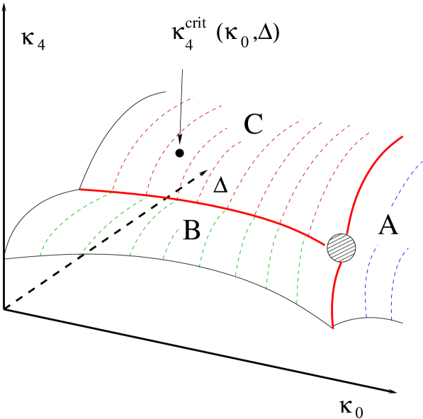
Figure 5: The phases A, B and C in the coupling constant space $(\kappa_{0},\Delta,\kappa_{4})$. Phase C is the one where extended four-dimensional geometries emerge.

We have performed extensive Monte Carlo simulations of the partition function $Z$ for a number of values of the bare coupling constants. As reported in blp , there are regions of the coupling constant space which do not appear relevant for continuum physics in that they seem to suffer from problems similar to the ones found earlier in Euclidean quantum gravity constructed in terms of dynamical triangulations, which essentially led to its abandonment in $d>2$. What is observed in Euclidean four-dimensional quantum gravity is the following: when the (inverse, bare) gravitational coupling $\kappa_{0}$ is sufficiently large one sees so-called branched polymers, i.e. not really a four-dimensional universe, but a universe which branches out like a tree with so many branches that it becomes truly fractal when the number of four-simplices becomes infinite, and its Hausdorff dimension is 2. Such triangulations represent the most extended triangulations one can construct unless one explicitly forbids branching. When the (inverse, bare) gravitational coupling $\kappa_{0}$ is sufficiently small one observes a totally crumpled universe with almost no extension. In this phase there exist vertices of very high order and the connectivity of the triangulation is such that it is possible to move from any four-simplex to any other crossing only a few neighbouring four-simplices. The Hausdorff dimension of such a triangulation is infinite in the limit where the number of four-simplices goes to infinity. These two phases, the crumpled and the branched polymer phase, are separated by a phase transition line along which there is a first-order transition. It was originally hoped that one could find a point on the critical line where the first-order transition becomes second order and which could then be used as a fixed point where a continuum theory of quantum gravity could be defined along the lines suggested by eqs. (10) and (11). However, such a second-order transition was not foundfirstorder , and eventuallythe idea of a theory of four-dimensional Euclidean quantum gravity was abandoned. A new principle for selecting the class of geometries one should use in the path integral was needed and this led to the suggestion to include only causal triangulations in the sum over spacetime histories.

When we include only the causal triangulations in the path integral, we still see a remnant of the Euclidean structure just described, namely, when the (inverse, bare) gravitational coupling $\kappa_{0}$ is sufficiently large, the Monte Carlo simulations exhibit a sequence in time direction of small, disconnected universes, none of them showing any sign of the scaling one would expect from a macroscopic universe. We denote this phase by A. We believe that this phase of the system is a Lorentzian version of the branched-polymer phase of Euclidean quantum gravity. By contrast, when $\Delta$ is sufficiently small, the simulations reveal a universe with a vanishing temporal extension of only a few lattice spacings, ending both in past and future in a vertex of very high order, connected to a large fraction of all vertices. This phase is most likely related to the so-called crumpled phase of Euclidean quantum gravity. We denote this phase by B. The crucial and new feature of the quantum superposition in terms of causal dynamical triangulations is the appearance of a region in coupling constant space which is different and interesting and where continuum physics may emerge. It is in this region that we have performed the simulations discussed here and where work up to now has already uncovered a number of intriguing physical results emerge ; semi ; blp ; spectral . In Fig. 6 we have shown how different configurations look in the three phases discussed above, and in Fig. 5 we have shown the tentative phase diagram in the coupling constant space of $\kappa_{0},\kappa_{4}$ and $\Delta$. A “critical” surface is shown in the figure. Keeping $\kappa_{0}$ and $\Delta$ fixed, $\kappa_{4}$ acts as a chemical potential for $N_{4}$; the smaller $\kappa_{4}$, the larger $\langle N_{4}\rangle$. At some critical value $\kappa_{4}(\kappa_{0},\Delta)$, depending on the choice of $\kappa_{0}$ and $\Delta$, $\langle N_{4}\rangle\to\infty$. For $\kappa_{4}<\kappa_{4}(\kappa_{0},\Delta)$ the partition function is plainly divergent and not defined. When we talk about phase transitions we are always at the “critical” surface

$$\kappa_{4}=\kappa_{4}(\kappa_{0},\Delta),$$ (16)

simply because we cannot have a phase transition unless $N_{4}=\infty$. We put “critical” into quotation marks since it only means that we probe infinite four-volume. No continuum limit is necessarily associated with a point on this surface. To decide this issue requires additional investigation. A good analogy is the Ising model on a finite lattice. To have a genuine phase transition for the Ising model we have to take the lattice volume to infinity since there are no genuine phase transitions for finite systems. However, just taking the lattice volume to infinity is not sufficient to ensure critical behaviour of the Ising model. We also have to tune the coupling constant to its critical value. Being on the “critical” surface, or rather “infinite-volume” surface (16), we can discuss various phases, and these are the ones indicated in the figure. The different phases are separated by phase transitions, which might be first-order. However, we have not yet conducted a systematic investigation of the order of the transitions. Looking at Fig. 5, we have two lines of phase transitions, separating phase A and phase C and separating phase B and phase C respectively. They meet in the point indicated on the figure. It is tempting to speculate that this point might be associated with a higher-order transition, as is common for statistical systems in such a situation. We will return to this point later.

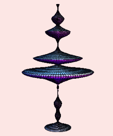
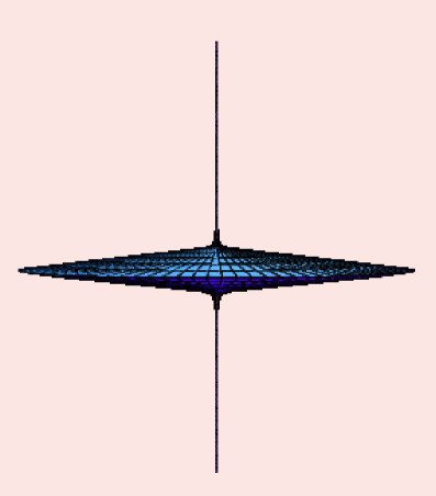
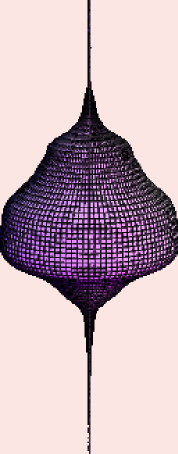
Figure 6: Typical configurations in the phases A, B and C (lowest figure). Phase C is the one where extended four-dimensional geometries emerge.

In the Euclideanized setting the value of the cosmological constant determines the spacetime volume $V_{4}$ since the two appear in the action as conjugate variables. We therefore have $\langle V_{4}\rangle\sim G/\Lambda$ in a continuum notation, where $G$ is the gravitational coupling constant and $\Lambda$ the cosmological constant. In the computer simulations it is more convenient to keep the four-volume fixed or partially fixed. We will implement this by fixing the total number of four-simplices of type $N_{4}^{(4,1)}$ or, equivalently, the total number $N_{3}$ of tetrahedra making up the spatial $S^{3}$ triangulations at times $t_{i}$, $i=1,\dots,N$,

$$N_{3}=\sum_{i=1}^{N}N_{3}(t_{i})=\frac{1}{2}N_{4}^{(4,1)}.$$ (17)

We know from the simulations that in the phase of interest $\langle N_{4}^{(4,1)}\rangle\propto\langle N_{4}^{(3,2)}\rangle$ as the total volume is varied blp . This effectively implies that we only have two bare coupling constants $\kappa_{0},\Delta$ in (15), while we compensate by hand for the coupling constant $\kappa_{4}$ by studying the partition function $Z(\kappa_{0},\Delta;N_{4}^{(4,1)})$ for various $N_{4}^{(4,1)}$. To keep track of the ratio $\xi(\kappa_{0},\Delta)$ between the expectation value $\langle N_{4}^{(3,2)}\rangle$ and $N_{4}^{(4,1)}$, which depends weakly on the coupling constants, we write (c.f. eq. (14))

$$\langle N_{4}\rangle=N_{4}^{(4,1)}+\langle N_{4}^{(3,2)}\rangle=N_{4}^{(4,1)}(1+\xi(\kappa_{0},\Delta)).$$ (18)

For all practical purposes we can regard $N_{4}$ in a Monte Carlo simulation as fixed. The relation between the partition function we use and the partition function with variable four-volume is given by the Laplace transformation

$$Z(\kappa_{0},\kappa_{4},\Delta)=\int_{0}^{\infty}\mbox{d}N_{4}\;\mbox{e}^{-\kappa_{4}N_{4}}\;Z(\kappa_{0},N_{4},\Delta),$$ (19)

where strictly speaking the integration over $N_{4}$ should be replaced by a summation over the discrete values $N_{4}$ can take. Returning to Fig. 5, keeping $N_{4}$ fixed rather than fine-tuning $\kappa_{4}$ to the critical value $\kappa_{4}^{c}$ implies that one is already on the “critical” surface drawn in Fig. 5, assuming that $N_{4}$ is sufficiently large (in principle infinite). Whether $N_{4}$ is sufficiently large to qualify as “infinite” can be investigated by performing the computer simulations for different $N_{4}$’s and comparing the results. This is a technique we will use over and over again in the following.

3 Numerical results

The Monte Carlo simulations referred to above will generate a sequence of spacetime histories. An individual spacetime history is not an observable, in the same way as a path $x(t)$ of a particle in the quantum-mechanical path integral is not. However, it is perfectly legitimate to talk about the expectation value $\langle x(t)\rangle$ as well as the fluctuations around $\langle x(t)\rangle$. Both of these quantities are in principle calculable in quantum mechanics. Let us make a slight digression and discuss this in some detail since it illustrates well the picture we also hope emerges in a theory of quantum gravity. Consider the particle example shown in Fig. 3. We have a particle moving from $x_{i}$ at $t_{i}$ to $x_{f}$ at $t_{f}$. In general there will be a classical motion of the particle satisfying these boundary conditions (we will assume that for simplicity). If $\hbar$ can be considered small compared to the other parameters entering into the description of the system, the classical path will be a good approximation to $\langle x(t)\rangle$ according to Ehrenfest’s theorem. In Fig. 3 the smooth curve represents $\langle x(t)\rangle$. In the path integral we sum over all continuous paths from $(x_{i},t_{i})$ to $(x_{f},t_{f})$ as illustrated in Fig. 3. However, when all other parameters in the problem are large compared to $\hbar$ we expect a “typical” path to be close to $\langle x(t)\rangle$ which also will be close to the classical path. Let us make this explicit in the simple case of the harmonic oscillator. Let $x_{cl}(t)$ denote the solution to the classical equations of motion such that $x_{cl}(t_{i})=x_{i}$ and $x_{cl}(t_{f})=x_{f}$. For the harmonic oscillator the decomposition

$$x(t)=x_{cl}(t)+y(t),~{}~{}~{}~{}y(t_{i})=y(t_{f})=0$$

leads to an exact factorization of the path integral thanks to the quadratic nature of the action. The part involving $x_{cl}(t)$ gives precisely the classical action and the part involving $y(t)$ the contributions from the fluctuations, independent of the classical part. Taking the classical path to be macroscopic gives a picture of a macroscopic path dressed with small quantum fluctuations, small because they are independent of the classical motion. Explicitly we have for the fluctuations (Euclidean calculation):

$$\left\langle\int_{t_{i}}^{t_{f}}\mbox{d}t\;y^{2}(t)\right\rangle=\frac{\hbar}{2m\omega^{2}}\;\left(\frac{\omega(t_{f}-t_{i})}{\tanh(\omega(t_{f}-t_{i}))}-1\right).$$

Thus the harmonic oscillator is a simple example of what we hope for in quantum gravity: Let the size of the system be macroscopic, i.e. $x_{cl}(t)$ is macroscopic (put in by hand): then the quantum fluctuations around this path are small and of the order

$$\langle|y|\rangle\propto\sqrt{\frac{\hbar}{m\omega^{2}(t_{f}-t_{i})}}.$$

We hope this translates into the description of our universe: the macroscopic size of the universe dictated by the (inverse) cosmological constant in any Euclidean description (trivial to show in the model by simply differentiating the partition function with respect to the cosmological constant and in the simulations thus put in by hand) and the small quantum fluctuations dictated by the other coupling constant, namely, the gravitational coupling constant.

3.1 The emergent de Sitter background

Obviously, there are many more dynamical variables in quantum gravity than there are in the particle case. We can still imitate the quantum-mechanical situation by picking out a particular one, for example, the spatial three-volume $V_{3}(t)$ at proper time $t$. We can measure both its expectation value $\langle V_{3}(t)\rangle$ as well as fluctuations around it. The former gives us information about the large-scale “shape” of the universe we have created in the computer. First we will describe the measurements of $\langle V_{3}(t)\rangle$, keeping a more detailed discussion of the fluctuations to Sec. 3.2 below.

A “measurement” of $V_{3}(t)$ consists of a table $N_{3}(i)$, where $i=1,\ldots,N$ denotes the number of time-slices. Recall from Sec. 2 that the sum over slices $\sum_{i=1}^{N}N_{3}(i)$ is kept constant. The time axis has a total length of $N$ time steps, where $N=80$ in the actual simulations, and we have cyclically identified time-slice $N+1$ with time-slice 1.

What we observe in the simulations is that for the range of discrete volumes $N_{4}$ under study the universe does not extend (i.e. has appreciable three-volume) over the entire time axis, but rather is localized in a region much shorter than 80 time slices. Outside this region the spatial extension $N_{3}(i)$ will be minimal, consisting of the minimal number (five) of tetrahedra needed to form a three-sphere $S^{3}$, plus occasionally a few more tetrahedra. This thin “stalk” therefore carries little four-volume and in a given simulation we can for most practical purposes consider the total four-volume of the remainder, the extended universe, as fixed.

In order to perform a meaningful average over geometries which explicitly refers to the extended part of the universe, we have to remove the translational zero mode which is present. We refer to bigs4 for a discussion of the procedure. Having defined the centre of volume along the time-direction of our spacetime configurations we can now perform superpositions of configurations and define the average $\langle N_{3}(i)\rangle$ as a function of the discrete time $i$. The results of measuring the average discrete spatial size of the universe at various discrete times $i$ are illustrated in Fig. 7 and can be succinctly summarized by the formula

$$N_{3}^{cl}(i):=\langle N_{3}(i)\rangle=\frac{N_{4}}{2(1+\xi)}\;\frac{3}{4}\frac{1}{s_{0}N_{4}^{1/4}}\cos^{3}\left(\frac{i}{s_{0}N_{4}^{1/4}}\right),~{}~{}~{}s_{0}\approx 0.59,$$ (20)

where $N_{3}(i)$ denotes the number of three-simplices in the spatial slice at discretized time $i$ and $N_{4}$ the total number of four-simplices in the entire universe. Since we are keeping $N_{4}^{(4,1)}$ fixed in the simulations and since $\xi$ changes with the choice of bare coupling constants, it is sometimes convenient to rewrite (20) as

$$N_{3}^{cl}(i)=\frac{1}{2}N_{4}^{(4,1)}\;\frac{3}{4}\frac{1}{\tilde{s}_{0}(N_{4}^{(4,1)})^{1/4}}\cos^{3}\left(\frac{i}{\tilde{s}_{0}(N_{4}^{(4,1)})^{1/4}}\right),$$ (21)

where $\tilde{s}_{0}$ is defined by $\tilde{s}_{0}(N_{4}^{(4,1)})^{1/4}=s_{0}N_{4}^{1/4}$. Of course, formula (20) is only valid in the extended part of the universe where the spatial three-volumes are larger than the minimal cut-off size.

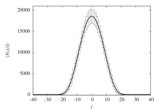
Figure 7: Background geometry $\langle N_{3}(i)\rangle$: MC measurements for fixed $N_{4}^{(4,1)}=160.000$ ($N_{4}=362.000$) and best fit (20) yield indistinguishable curves at given plot resolution. The bars indicate the average size of quantum fluctuations.

The data shown in Fig. 7 have been collected at the particular values $(\kappa_{0},\Delta)=(2.2,0.6)$ of the bare coupling constants and for $N_{4}=362.000$ (corresponding to $N_{4}^{(4,1)}=160.000$). For this value of $(\kappa_{0},\Delta)$ we have verified relation (20) for $N_{4}$ ranging from 45.500 to 362.000 building blocks (45.500, 91.000, 181.000 and 362.000). After rescaling the time and volume variables by suitable powers of $N_{4}$ according to relation (20), and plotting them in the same way as in Fig. 7, one finds almost total agreement between the curves for different spacetime volumes. This is illustrated in Fig. 8. Thus we have here a beautiful example of finite-size scaling, and at least when we discuss the average three-volume $V_{3}(t)$ all our discretized volumes $N_{4}$ are large enough that we can treat them as infinite, in the sense that no further change will occur for larger $N_{4}$.

By contrast, the quantum fluctuations indicated in Fig. 7 as vertical bars are volume-dependent and will be the larger the smaller the total four-volume, see Sec. 3.2 below for details. eq. (20) shows that spatial volumes scale according to $N_{4}^{3/4}$ and time intervals according to $N_{4}^{1/4}$, as one would expect for a genuinely four-dimensional spacetime and this is exactly the scaling we have used in Fig. 8. This strongly suggests a translation of (20) to a continuum notation. The most natural identification is given by

$$\sqrt{g_{tt}}\;V_{3}^{cl}(t)=V_{4}\;\frac{3}{4B}\cos^{3}\left(\frac{t}{B}\right),$$ (22)

where we have made the identifications

$$\frac{t_{i}}{B}=\frac{i}{s_{0}N_{4}^{1/4}},~{}~{}~{}~{}\Delta t_{i}\sqrt{g_{tt}}\;V_{3}(t_{i})=2{\tilde{C}}_{4}N_{3}(i)a^{4},$$ (23)

such that we have

$$\int dt\sqrt{g_{tt}}\;V_{3}(t)=V_{4}.$$ (24)

In (23), $\sqrt{g_{tt}}$ is the constant proportionality factor between the time $t$ and genuine continuum proper time $\tau$, $\tau=\sqrt{g_{tt}}\;t$. (The combination $\Delta t_{i}\sqrt{g_{tt}}V_{3}$ contains ${\tilde{C}}_{4}$, related to the four-volume of a four-simplex rather than the three-volume corresponding to a tetrahedron, because its time integral must equal $V_{4}$). Writing $V_{4}=8\pi^{2}R^{4}/{3}$, and $\sqrt{g_{tt}}=R/B$, eq. (22) is seen to describe a Euclidean de Sitter universe (a four-sphere, the maximally symmetric space for positive cosmological constant) as our searched-for, dynamically generated background geometry! In the parametrization of (22) this is the classical solution to the action

$$S=\frac{1}{24\pi G}\int dt\sqrt{g_{tt}}\left(\frac{g^{tt}\dot{V_{3}}^{2}(t)}{V_{3}(t)}+k_{2}V_{3}^{1/3}(t)-\lambda V_{3}(t)\right),$$ (25)

where $k_{2}=9(2\pi^{2})^{2/3}$ and $\lambda$ is a Lagrange multiplier, fixed by requiring that the total four-volume be $V_{4}$, $\int dt\sqrt{g_{tt}}\;V_{3}(t)=V_{4}$. Up to an overall sign, this is precisely the Einstein-Hilbert action for the scale factor $a(t)$ of a homogeneous, isotropic universe (rewritten in terms of the spatial three-volume $V_{3}(t)=2\pi^{2}a(t)^{3}$), although we of course never put any such simplifying symmetry assumptions into the CDT model.

\psfrag{t}{{\bf{\large$\sigma$}}}\psfrag{v}{{\bf{\large$P(\sigma)$}}}\includegraphics{semi.eps}

Figure 8: Rescaling of time and volume variables according to relation (20) for $N_{4}=$ 45.500, 91.000, 181.000 and 362.000. The plot also include the curve (20). More precisely: $\sigma\propto i/N_{4}^{1/4}$ and $P(\sigma)\propto N_{3}(i)/N_{4}^{3/4}$.

A discretized, dimensionless version of (25) is

$$S_{discr}=k_{1}\sum_{i}\left(\frac{(N_{3}(i+1)-N_{3}(i))^{2}}{N_{3}(i)}+\tilde{k}_{2}N_{3}^{1/3}(i)\right),$$ (26)

where $\tilde{k}_{2}\propto k_{2}$. This can be seen by applying the scaling (20), namely, $N_{3}(i)=N_{4}^{3/4}n_{3}(s_{i})$ and $s_{i}=i/N_{4}^{1/4}$. This enables us to finally conclude that the identifications (23) when used in the action (26) lead naïvely to the continuum expression (25) under the identification

$$G=\frac{a^{2}}{k_{1}}\frac{\sqrt{{\tilde{C}}_{4}}\;{\tilde{s}}_{0}^{2}}{3\sqrt{6}}.$$ (27)

Next, let us comment on the universality of these results. First, we have checked that they are not dependent on the particular definition of time-slicing we have been using, in the following sense. By construction of the piecewise linear CDT-geometries we have at each integer time step $t_{i}=i\,a_{t}$ a spatial surface consisting of $N_{3}(i)$ tetrahedra. Alternatively, one can choose as reference slices for the measurements of the spatial volume non-integer values of time, for example, all time slices at discrete times $i-1/2$, $i=1,2,...$ . In this case the “triangulation” of the spatial three-spheres consists of tetrahedra – from cutting a (4,1)- or a (1,4)-simplex half-way – and “boxes”, obtained by cutting a (2,3)- or (3,2)-simplex (the geometry of this is worked out in dl ). We again find a relation like (20) if we use the total number of spatial building blocks in the intermediate slices (tetrahedra+boxes) instead of just the tetrahedra.

Second, we have repeated the measurements for other values of the bare coupling constants. As long as we stay in the phase where an extended universe is observed, the phase C in Fig. 5, a relation like (20) remains valid. In addition, the value of $s_{0}$, defined in eq. (20), is almost unchanged until we get close to the phase transition lines beyond which the extended universe disappears. Only for the values of $\kappa_{0}$ around 3.6 and larger will the measured $\langle N_{3}(t)\rangle$ differ significantly from the value at 2.2. For values larger than 3.8 (at $\Delta=0.6$), the universe will disintegrate into a number of small and disconnected components distributed randomly along the time axis, and one can no longer fit the distribution $\langle N_{3}(t)\rangle$ to the formula (20). Later we will show that while $s_{0}$ is almost unchanged, the constant $k_{1}$ in (26), which governs the quantum fluctuations around the mean value $\langle N_{3}(t)\rangle$, is more sensitive to a change of the bare coupling constants, in particular, in the case where we change $\kappa_{0}$ (while leaving $\Delta$ fixed).

3.2 Fluctuations around de Sitter space

In the following we will test in more detail how well the actions (25) and (26) describe the computer data. A crucial test is how well it describes the quantum fluctuations around the emergent de Sitter background.

The correlation function (the covariance matrix ${\hat{C}}$) is defined by

$$C_{N_{4}}(i,i^{\prime})=\langle\delta N_{3}(i)\delta N_{3}(i^{\prime})\rangle,~{}~{}~{}~{}\delta N_{3}(i)\equiv N_{3}(i)-{\bar{N}}_{3}(i),$$ (28)

where we have included an additional subscript $N_{4}$ to emphasize that $N_{4}$ is kept constant in a given simulation.

The first observation extracted from the Monte Carlo simulations is that under a change in the four-volume $C_{N_{4}}(i,i^{\prime})$ scales as

$$C_{N_{4}}(i,i^{\prime})=N_{4}\;F\Big{(}{i}/N^{1/4}_{4},{i^{\prime}}/N_{4}^{1/4}\Big{)},$$ (29)

where $F$ is a universal scaling function.

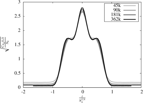
Figure 9: Analyzing the quantum fluctuations of Fig. 7: diagonal entries $F(t,t)^{1/2}$ of the universal scaling function $F$ from (29), for $N_{4}^{(4,1)}=$ 20.000, 40.000, 80.000 and 160.000.

This is illustrated by Fig. 9 for the rescaled version of the diagonal part $C_{N_{4}}^{1/2}(i,i)$, corresponding precisely to the quantum fluctuations $\langle(\delta N_{3}(i))^{2}\rangle^{1/2}$ of Fig. 7. While the height of the curve in Fig. 7 will grow as $N_{4}^{3/4}$, the superimposed fluctuations will only grow as $N_{4}^{1/2}$. We conclude that for fixed bare coupling constants the relative fluctuations will go to zero in the infinite-volume limit .

Let us rewrite the minisuperspace action (25) for a fixed, finite four-volume $V_{4}$ in terms of dimensionless variables by introducing $s=t/V_{4}^{1/4}$ and $V_{3}(t)=V_{4}^{3/4}v_{3}(s)$:

$$S=\frac{1}{24\pi}\;\frac{\sqrt{V_{4}}}{G}\int ds\sqrt{g_{ss}}\left(\frac{g^{ss}\dot{v_{3}}^{2}(s)}{v_{3}(s)}+k_{2}v_{3}^{1/3}(s)\right),$$ (30)

now assuming that $\int ds\sqrt{g_{ss}}\;v_{3}(s)=1$, and with $g_{ss}\equiv g_{tt}$. The same rewriting can be done to (26) which becomes

$$S_{discr}=k_{1}\sqrt{N_{4}}\sum_{i}\Delta s\left(\frac{1}{n_{3}(s_{i})}\left(\frac{n_{3}(s_{i+1})-n_{3}(s_{i})}{\Delta s}\right)^{2}+\tilde{k}_{2}n_{3}^{1/3}(s_{i})\right),$$ (31)

where $N_{3}(i)=N_{4}^{3/4}n_{3}(s_{i})$ and $s_{i}=i/N_{4}^{1/4}$.

From the way the factor $\sqrt{N_{4}}$ appears as an overall scale in eq. (31) it is clear that to the extent a quadratic expansion around the effective background geometry is valid one will have a scaling

$$\langle\delta N_{3}(i)\delta N_{3}(i^{\prime})\rangle=N_{4}^{3/2}\langle\delta n_{3}(t_{i})\delta n_{3}(t_{i^{\prime}})\rangle=N_{4}F(t_{i},t_{i^{\prime}}),$$ (32)

where $t_{i}=i/N_{4}^{1/4}$. This implies that (29) provides additional evidence for the validity of the quadratic approximation and the fact that our choice of action (26), with $k_{1}$ independent of $N_{4}$ is indeed consistent.

To demonstrate in detail that the full function $F(t,t^{\prime})$ and not only its diagonal part is described by the effective actions (25), (26), let us for convenience adopt a continuum language and compute its expected behaviour. Expanding (25) around the classical solution according to $V_{3}(t)=V_{3}^{cl}(t)+x(t)$, the quadratic fluctuations are given by

$$\langle x(t)x(t^{\prime})\rangle \!=\! \int{\cal D}x(s)\;x(t)x(t^{\prime})\;e^{-\frac{1}{2}\int\!\!\int dsds^{\prime}x(s)M(s,s^{\prime})x(s^{\prime})}$$ (33)

$$\!=\! M^{-1}(t,t^{\prime}),$$

where ${\cal D}x(s)$ is the normalized measure and the quadratic form $M(t,t^{\prime})$ is determined by expanding the effective action $S$ to second order in $x(t)$,

$$S(V_{3})=S(V_{3}^{cl})+\frac{1}{18\pi G}\frac{B}{V_{4}}\int\mbox{d}t\;x(t){\hat{H}}x(t).$$ (34)

In expression (34), ${\hat{H}}$ denotes the Hermitian operator

$${\hat{H}}=-\frac{\mbox{d}}{\mbox{d}t}\frac{1}{\cos^{3}(t/B)}\frac{\mbox{d}}{\mbox{d}t}-\frac{4}{B^{2}\cos^{5}(t/B)},$$ (35)

which must be diagonalized under the constraint that $\int dt\sqrt{g_{tt}}\;x(t)=0$, since $V_{4}$ is kept constant.

Let $e^{(n)}(t)$ be the eigenfunctions of the quadratic form given by (34) with the volume constraint enforced, ordered according to increasing eigenvalues $\lambda_{n}$. As we will discuss shortly, the lowest eigenvalue is $\lambda_{1}=0$, associated with translational invariance in time direction, and should be left out when we invert $M(t,t^{\prime})$, because we precisely fix the centre of volume when making our measurements. Its dynamics is therefore not accounted for in the correlator $C(t,t^{\prime})$.

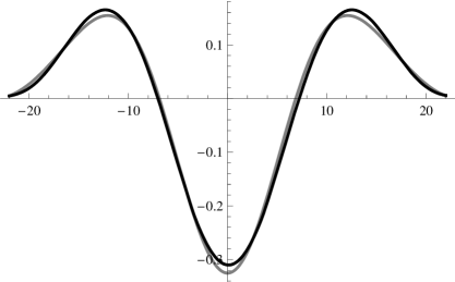
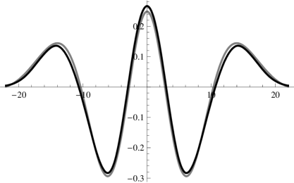
Figure 10: Comparing the two highest even eigenvector of the covariance matrix $C(t,t^{\prime})$ measured directly (gray curves) with the two lowest even eigenvectors of $M^{-1}(t,t^{\prime})$, calculated semi-classically (black curves).

If this cosmological continuum model were to give the correct description of the computer-generated universe, the matrix

$$M^{-1}(t,t^{\prime})=\sum_{n=2}^{\infty}\frac{e^{(n)}(t)e^{(n)}(t^{\prime})}{\lambda_{n}}$$ (36)

should be proportional to the measured correlator $C(t,t^{\prime})$. Fig. 10 shows the eigenfunctions $e^{(2)}(t)$ and $e^{(4)}(t)$ (with two and four zeros respectively), calculated from ${\hat{H}}$ with the constraint $\int dt\sqrt{g_{tt}}\;x(t)=0$ imposed. Simultaneously we show the corresponding eigenfunctions calculated from the data, i.e. from the matrix $C(t,t^{\prime})$, which correspond to the (normalizable) eigenfunctions with the highest and third-highest eigenvalues. The agreement is very good, in particular, when taking into consideration that no parameter has been adjusted in the action (we simply take $B=s_{0}N_{4}^{1/4}\Delta t$ in (22) and (34), which gives $B=14.47a_{t}$ for $N_{4}=362.000$).

The reader may wonder why the first eigenfunction exhibited has two zeros. As one would expect, the ground state eigenfunction $e^{(0)}(t)$ of the Hamiltonian (35), corresponding to the lowest eigenvalue, has no zeros, but it does not satisfy the volume constraint $\int dt\sqrt{g_{tt}}\;x(t)=0$. The eigenfunction $e^{(1)}(t)$ of ${\hat{H}}$ with next-lowest eigenvalue has one zero and is given by the simple analytic function

$$e^{(1)}(t)=\frac{4}{\sqrt{\pi B}}\sin\Big{(}\frac{t}{B}\Big{)}\,\cos^{2}\Big{(}\frac{t}{B}\Big{)}=c^{-1}\frac{dV_{3}^{cl}(t)}{dt},$$ (37)

where $c$ is a constant. One realizes immediately that $e^{(1)}$ is the translational zero mode of the classical solution $V_{3}^{cl}(t)$ ($\propto\cos^{3}t/B$). Since the action is invariant under time translations, we have

$$S(V_{3}^{cl}(t+\Delta t))=S(V_{3}^{cl}(t)),$$ (38)

and since $V_{3}^{cl}(t)$ is a solution to the classical equations of motion we find to second order (using the definition (37))

$$S(V_{3}^{cl}(t+\Delta t))=S(V_{3}^{cl}(t))+\frac{c^{2}(\Delta t)^{2}}{18\pi G}\frac{B}{V_{4}}\int dt\;e^{(1)}(t){\hat{H}}e^{(1)}(t),$$ (39)

consistent with $e^{(1)}(t)$ having eigenvalue zero.

It is clear from Fig. 10 that some of the eigenfunctions of ${\hat{H}}$ (with the volume constraint imposed) agree very well with the measured eigenfunctions. All even eigenfunctions (those symmetric with respect to reflection about the symmetry axis located at the centre of volume) turn out to agree very well. The odd eigenfunctions of ${\hat{H}}$ agree less well with the eigenfunctions calculated from the measured $C(t,t^{\prime})$. The reason seems to be that we have not managed to eliminate the motion of the centre of volume completely from our measurements. There is an inherent ambiguity in fixing the centre of volume of one lattice spacing, which turns out to be sufficient to reintroduce the zero mode in the data. Suppose we had by mistake misplaced the centre of volume by a small distance $\Delta t$. This would introduce a modification

$$\Delta V_{3}=\frac{dV_{3}^{cl}(t)}{dt}\;\Delta t$$ (40)

proportional to the zero mode of the potential $V_{3}^{cl}(t)$. It follows that the zero mode can re-enter whenever we have an ambiguity in the position of the centre of volume. In fact, we have found that the first odd eigenfunction extracted from the data can be perfectly described by a linear combination of $e^{(1)}(t)$ and $e^{(3)}(t)$. It may be surprising at first that an ambiguity of one lattice spacing can introduce a significant mixing. However, if we translate $\Delta V_{3}$ from eq. (40) to “discretized” dimensionless units using $V_{3}(i)\sim N_{4}^{3/4}\cos(i/N_{4}^{1/4})$, we find that $\Delta V_{3}\sim\sqrt{N_{4}}$, which because of $\langle(\delta N_{3}(i))^{2}\rangle\sim N_{4}$ is of the same order of magnitude as the fluctuations themselves. In our case, this apparently does affect the odd eigenfunctions.

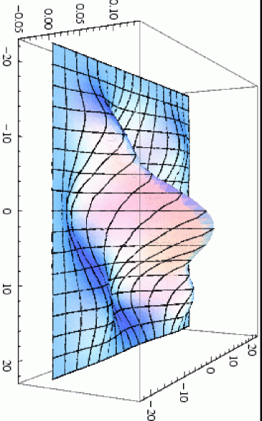
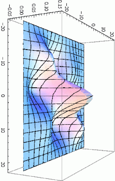
Figure 11: Comparing data for the extended part of the universe: measured $C(t,t^{\prime})$ (above) versus $M^{-1}(t,t^{\prime})$ obtained from analytical calculation (below). The agreement is good, and would have been even better had we included only the even modes.

One can also compare the data and the matrix $M^{-1}(t,t^{\prime})$ calculated from (36) directly. This is illustrated in Fig. 11, where we have restricted ourselves to data from inside the extended part of the universe. We imitate the construction (36) for $M^{-1}$, using the data to calculate the eigenfunctions, rather than ${\hat{H}}$. One could also have used $C(t,t^{\prime})$ directly, but the use of the eigenfunctions makes it somewhat easier to perform the restriction to the bulk. The agreement is again good (better than 15% at any point on the plot), although less spectacular than in Fig. 10 because of the contribution of the odd eigenfunctions to the data.

3.3 The size of the universe and the flow of $G$

It is natural to view the coupling constant $G$ in front of the effective action for the scale factor as the gravitational coupling constant $G$. The effective action which described our computer-generated data was given by eq. (25) and its dimensionless lattice version by (26). The computer data allows us to extract $k_{1}\propto a^{2}/G$, $a$ being the spatial lattice spacing, the precise constant of proportionality being given by eq. (27):

$${G}=\frac{a^{2}}{k_{1}}\frac{\sqrt{{\tilde{C}}_{4}}\;{\tilde{s}}_{0}^{2}}{3\sqrt{6}}.$$ (41)

For the bare coupling constants $(\kappa_{0},\Delta)=(2.2,0.6)$ we have high-statistics measurements for $N_{4}$ ranging from 45.500 to 362.000 four-simplices (equivalently, $N_{4}^{(4,1)}$ ranging from 20.000 to 160.000 four-simplices). The choice of $\Delta$ determines the asymmetry parameter $\alpha$, and the choice of $(\kappa_{0},\Delta)$ determines the ratio $\xi$ between $N_{4}^{(3,2)}$ and $N_{4}^{(4,1)}$. This in turn determines the “effective” four-volume ${\tilde{C}}_{4}$ of an average four-simplex, which also appears in (41). The number ${\tilde{s}}_{0}$ in (41) is determined directly from the time extension $T_{\rm univ}$ of the extended universe according to

$$T_{\rm univ}=\pi\;{\tilde{s}}_{0}\Big{(}N_{4}^{(4,1)}\Big{)}^{1/4}.$$ (42)

Finally, from our measurements we have determined $k_{1}=0.038$. Taking everything together according to (41), we obtain $G\approx 0.23a^{2}$, or $\ell_{Pl}\approx 0.48a$, where $\ell_{Pl}=\sqrt{G}$ is the Planck length.

From the identification of the volume of the four-sphere, $V_{4}=8\pi^{2}R^{4}/{3}={\tilde{C}}_{4}N_{4}^{(4,1)}a^{4}$, we obtain that $R=3.1a$. In other words, the linear size $\pi R$ of the quantum de Sitter universes studied here lies in the range of 12-21 Planck lengths for $N_{4}$ in the range mentioned above and for the bare coupling constants chosen as $(\kappa_{0},\Delta)=(2.2,0.6)$.

Our dynamically generated universes are therefore not very big, and the quantum fluctuations around their average shape are large as is apparent from Fig. 7. It is rather surprising that the semi-classical minisuperspace formulation is applicable for universes of such a small size, a fact that should be welcome news to anyone performing semi-classical calculations to describe the behaviour of the early universe. However, in a certain sense our lattices are still coarse compared to the Planck scale $\ell_{Pl}$ because the Planck length is roughly half a lattice spacing. If we are after a theory of quantum gravity valid on all scales, we are in particular interested in uncovering phenomena associated with Planck-scale physics. In order to collect data free from unphysical short-distance lattice artifacts at this scale, we would ideally like to work with a lattice spacing much smaller than the Planck length, while still being able to set by hand the physical volume of the universe studied on the computer.

The way to achieve this, under the assumption that the coupling constant $G$ of formula (41) is indeed a true measure of the gravitational coupling constant, is as follows. We are free to vary the discrete four-volume $N_{4}$ and the bare coupling constants $(\kappa_{0},\Delta)$ of the Regge action (see blp for further details on the latter). Assuming for the moment that the semi-classical minisuperspace action is valid, the effective coupling constant $k_{1}$ in front of it will be a function of the bare coupling constants $(\kappa_{0},\Delta)$, and can in principle be determined as described above for the case $(\kappa_{0},\Delta)=(2.2,0.6)$. If we adjusted the bare coupling constants such that in the limit as $N_{4}\to\infty$ both

$$V_{4}\sim N_{4}a^{4}~{}~{}~{}{\rm and}~{}~{}~{}G\sim a^{2}/k_{1}(\kappa_{0},\Delta)$$ (43)

remained constant (i.e. $k_{1}(\kappa_{0},\Delta)\sim 1/\sqrt{N_{4}}$), we would eventually reach a region where the Planck length was significantly smaller than the lattice spacing $a$, in which event the lattice could be used to approximate spacetime structures of Planckian size and we could initiate a genuine study of the sub-Planckian regime.

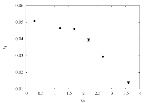
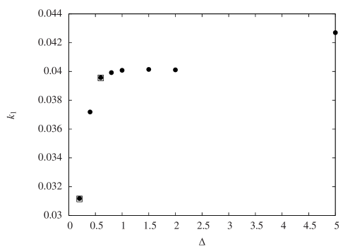
Figure 12: The measured effective coupling constant $k_{1}$ as function of the bare $\kappa_{0}$ (top, $\Delta=0.6$ fixed) and the asymmetry $\Delta$ (bottom, $\kappa_{0}=2.2$ fixed). The marked point near the middle of the data points sampled is the point $(\kappa_{0},\Delta)=(2.2,0.6)$ where most measurements in the remainder of the paper were taken. The other marked points are those closest to the two phase transitions, to the “branched-polymer phase” (top), and the “crumpled phase” (bottom).

Since we have no control over the effective coupling constant $k_{1}$, the first obvious question which arises is whether we can at all adjust the bare coupling constants in such a way that at large scales we still see a four-dimensional universe, with $k_{1}$ going to zero at the same time. The answer seems to be in the affirmative, as we will go on to explain.

Fig. 12 shows the results of extracting $k_{1}$ for a range of bare coupling constants for which we still observe an extended universe. In the top figure $\Delta=0.6$ is kept constant while $\kappa_{0}$ is varied. For $\kappa_{0}$ sufficiently large we eventually reach a point where a phase transition takes place (the point in the square in the bottom right-hand corner is the measurement closest to the transition we have looked at). For even larger values of $\kappa_{0}$, beyond this transition, the universe disintegrates into a number of small universes, in a CDT-analogue of the branched-polymer phase of Euclidean quantum gravity. The plot shows that the effective coupling constant $k_{1}$ becomes smaller and possibly goes to zero as the phase transition point is approached, although our current data do not yet allow us to conclude that $k_{1}$ does indeed vanish at the transition point.

Conversely, the bottom figure of Fig. 12 shows the effect of varying $\Delta$, while keeping $\kappa_{0}=2.2$ fixed. As $\Delta$ is decreased towards 0, we eventually hit another phase transition, separating the physical phase of extended universes from the CDT-equivalent of the crumpled phase of Euclidean quantum gravity, where the entire universe will be concentrated within a few time steps, as already mentioned above. (The point closest to the transition where we have taken measurements is the one in the bottom left-hand corner.) Also when approaching this phase transition the effective coupling constant $k_{1}$ goes to 0, leading to the tentative conclusion that $k_{1}\to 0$ along the entire phase boundary.

However, to extract the coupling constant $G$ from (41) we not only have to take into account the change in $k_{1}$, but also that in ${\tilde{s}}_{0}$ (the width of the distribution $N_{3}(i)$) and in the effective four-volume ${\tilde{C}}_{4}$ as a function of the bare coupling constants. Combining these changes, we arrive at a slightly different picture. Approaching the boundary where spacetime collapses in time direction (by lowering $\Delta$), the gravitational coupling constant $G$ decreases, despite the fact that $1/k_{1}$ increases. This is a consequence of ${\tilde{s}}_{0}$ decreasing considerably. On the other hand, when (by increasing $\kappa_{0}$) we approach the region where the universe breaks up into several independent components, the effective gravitational coupling constant $G$ increases, more or less like $1/k_{1}$, where the behaviour of $k_{1}$ is shown in Fig. 12 (top). This implies that the Planck length $\ell_{Pl}=\sqrt{G}$ increases from approximately $0.48a$ to $0.83a$ when $\kappa_{0}$ changes from 2.2 to 3.6. Most likely we can make it even bigger in terms of Planck units by moving closer to the phase boundary.

On the basis of these arguments, it seems likely that the non-perturbative CDT-formulation of quantum gravity does allow us to penetrate into the sub-Planckian regime and probe the physics there explicitly. Work in this direction is currently ongoing. One interesting issue under investigation is whether and to what extent the simple minisuperspace description remains valid as we go to shorter scales. We have already seen deviations from classicality at short scales when measuring the spectral dimension spectral ; blp , and one would expect them to be related to additional terms in the effective action (25) and/or a nontrivial scaling behaviour of $k_{1}$. This raises the interesting possibility of being able to test explicitly the scaling violations of $G$ predicted by renormalization group methods in the context of asymptotic safety reuteretc .

4 Two-dimensional Euclidean quantum gravity

The results described above are of course interesting and suggest that there might exist a field theory of quantum gravity in four dimensions (three space and one time dimension). However, the results are based on numerical simulations. As already mentioned it is of great conceptional interest that we have a toy model, two-dimensional quantum gravity, where both the lattice theory and the continuum quantum gravity theory can be solved analytically and agree. Of course we can still be in the situation that there exists no description of quantum gravity as a field theory in four dimensions (although we have presented some evidence in favour of such a scenario above), but we can then not blame the underlying formalism for being inadequate.

4.1 Continuum formulation

Let $M^{h}$ denote a closed, compact, connected and orientable surface of genus $h$ and Euler characteristic $\chi(h)=2-2h$. The partition function of two-dimensional Euclidean quantum gravity is formally given by

$$Z(\Lambda,G)=\sum_{h=0}^{\infty}\int{\cal D}[g]\,e^{-S(g;\Lambda,G)},$$ (44)

where $\Lambda$ denotes the cosmological constant, $G$ is the gravitational coupling constant and $S$ is the continuum Einstein–Hilbert action defined by

$$S(g;\Lambda,G)=\Lambda\int_{M^{h}}d^{2}\xi\sqrt{g}-\frac{1}{2\pi G}\int_{M^{h}}d^{2}\xi\sqrt{g}\,R.$$ (45)

In eq. (44), we take the sum to include all possible topologies of two-dimensional manifolds (i.e. over all genera $h$), and in eq. (45) $R$ denotes the scalar curvature of the metric $g$ on the manifold $M^{h}$. The functional integration is over all diffeomorphism equivalence classes $[g]$ of metrics on $M^{h}$.

In two dimensions the curvature part of the Einstein–Hilbert action is a topological invariant according to the Gauss–Bonnet theorem, which allows us to write

$$Z(\Lambda,G)=\sum_{h=0}^{\infty}e^{\chi(h)/G}Z_{h}(\Lambda),$$ (46)

where

$$Z_{h}(\Lambda)=\int{\cal D}[g]\,e^{-S(g;\Lambda)},$$ (47)

and

$$S(g;\Lambda)=\Lambda\,V_{g},$$ (48)

where $V_{g}=\int d^{2}\xi\,\sqrt{g}$ is the volume of the universe for a given diffeomorphism class of metrics. In the remainder of this section we will, for simplicity, restrict our attention to manifolds homeomorphic to $S^{2}$ or $S^{2}$ with a fixed number of holes unless explicitly stated otherwise. In this case we disregard the topological term in the action since it is a constant. The sphere $S^{2}$ with $b$ boundary components will be denoted $S^{2}_{b}$ and we denote the partition function for the sphere, $Z_{0}(\Lambda)$ in eq. (47), by $Z(\Lambda)$.

In the presence of a boundary it is natural to add to the action a boundary term

$$S(g;\Lambda,Z_{1},...,Z_{b})=\Lambda V_{g}+\!\sum_{i=1}^{b}Z_{i}L_{i,g},$$ (49)

where $L_{i,g}$ denotes the length of the $i$th boundary component with respect to the metric $g$. We refer to the $Z_{i}$’s as the cosmological constants of the boundary components. The partition function is in this case given by

$$W(\Lambda;Z_{1},...,Z_{b})=\int{\cal D}[g]\,e^{-S(g;\Lambda,Z_{1},\ldots,Z_{b})}.$$ (50)

Since the lengths of the boundary components are invariant under diffeomorphisms, it makes sense to fix them to values $L_{1},\ldots,L_{b}$ and define the Hartle–Hawking wave functionals by

$$W(\Lambda;L_{1},...,L_{b})=\int{\cal D}[g]\,e^{-S(g;\Lambda)}\,\prod_{i=1}^{b}\delta(L_{i}-L_{i,g}),$$ (51)

where $S(g;\Lambda)$ is given by eq. (48). Since eq. (50) is the Laplace transform of eq. (51), i.e.

$$W(\Lambda;Z_{1},...,Z_{b})=\int_{0}^{\infty}\prod_{i=1}^{b}dL_{i}\,e^{-Z_{i}L_{i}}\,W(\Lambda;L_{1},...,L_{b}),$$ (52)

we denote them by the same symbol. We distinguish between the two by the names of the arguments.

4.2 The lattice regularization

At the outset we restrict the topology of surfaces to be that of $S^{2}$ with a fixed number of holes. We view abstract triangulations of $S^{2}_{b}$ as defining a grid in the space of diffeomorphism equivalence classes of metrics on $S^{2}_{b}$. Each triangle is a “building block” with side lengths $a$. This $a$ will be a UV cut-off which we will relate to the bare coupling constants on the lattice. However, presently it is convenient to view $a$ as being 1 (length unit).

Let $T$ denote a triangulation of $S^{2}_{b}$. The regularized theory of gravity will be defined by replacing the action $S_{g}(\Lambda,Z_{1},\ldots,Z_{b})$ in eq. (49) by

$$S_{T}(\mu,\lambda_{1},\ldots,\lambda_{b})=\mu N_{t}+\sum_{i=1}^{b}\lambda_{i}l_{i},$$ (53)

where $N_{t}$ denotes the number of triangles in $T$ and $l_{i}$ is the number of links in the $i$th boundary component. The parameter $\mu$ is the bare cosmological constant and the $\lambda_{i}$’s are the bare cosmological constants of the boundary components. The integration over diffeomorphism equivalence classes of metrics in eq.  (50) becomes a summation over non-isomorphic triangulations. We define the loop functions (discretized versions of $W(\Lambda,Z_{1},\ldots,Z_{b})$) by summing over all triangulations of $S^{2}_{b}$:

$$w(\mu,\lambda_{1},\ldots,\lambda_{b})=\sum_{l_{1},\ldots,l_{b}}\,\sum_{T\in{\cal T}(l_{1},\ldots,l_{b})}\,e^{-S_{T}(\mu,\lambda_{1},\ldots,\lambda_{b})}.$$ (54)

Analogously, we define the partition function for closed surfaces by

$$Z(\mu)=\sum_{T\in{\cal T}}\frac{1}{C_{T}}\,e^{-S_{T}(\mu)},$$ (55)

where $C_{T}$ is the symmetry factor of $T$ and $S_{T}(\mu)=\mu N_{t}$. Since we consider surfaces of a fixed topology we have left out the curvature term in the action. It will be introduced later, when the restriction on topology is lifted.

Next we write down the regularized version of the Hartle–Hawking wave functionals $W(\Lambda,L_{1},\ldots,L_{b})$:

$$w(\mu,l_{1},\ldots,l_{b})=\sum_{T\in{\cal T}(l_{1},\ldots,l_{b})}e^{-S_{T}(\mu)}$$ (56)

with an abuse of notation similar to the one in the previous section. This can also be written in the form

$$w(\mu,l_{1},\ldots,l_{b})=\sum_{k}e^{-\mu k}w_{k,l_{1},\ldots,l_{b}}\;,$$ (57)

where we have introduced the notation

$$w_{k,l_{1},\ldots,l_{b}}$$

for the number of triangulations in ${\cal T}(l_{1},\ldots,l_{b})$ with $k$ triangles.

The discretized analogues of the Laplace transformations which relate $W(\Lambda,Z_{1},\ldots,Z_{b})$ and $W(\Lambda,L_{1},\ldots,L_{b})$ are

$$w(\mu,\lambda_{1},\ldots,\lambda_{b})=\sum_{l_{1},\ldots,l_{b}}e^{-\sum_{i}\lambda_{i}l_{i}}w(\mu,l_{1},\ldots,l_{b})$$ (58)

and eq. (57). Similarly, we have for the partition functions

$$Z(\mu) = \sum_{k}e^{-\mu k}Z(k),$$ (59)

$$Z(k) = \sum_{T\in{\cal T},N_{t}=k}\frac{1}{C_{T}}.$$ (60)

It follows from the definitions (57)–(58) that $w(\mu,\lambda_{1},\ldots,\lambda_{b})$ is the generating function for the numbers $w_{k,l_{1},\ldots,l_{b}}$, the arguments of the generating function being $e^{-\mu}$ and $e^{-\lambda_{i}}$. In this way the evaluation of the loop functions of two-dimensional quantum gravity is reduced to the purely combinatorial problem of finding the number of non-isomorphic triangulations of $S^{2}$ or $S^{2}_{b}$ with a given number of triangles and boundary components of given lengths.

We use the notation

$$w(g,z_{1},\ldots,z_{b})=\sum_{k,l_{1},\ldots,l_{b}}w_{k,l_{1},\ldots,l_{b}}\,g^{k}z_{1}^{-l_{1}-1}\cdots z_{b}^{-l_{b}-1}$$ (61)

for the generating function with an extra factor $z_{1}^{-1}\ldots z_{b}^{-1}$, i.e. we make the identifications

$$g=e^{-\mu},~{}~{}~{}~{}z_{i}=e^{\lambda_{i}}.$$ (62)

The reason for this particular choice of variables in the generating function is motivated by its analytic structure, which will be revealed below.

In the following we consider a particular class of triangulations

Figure 13: A typical unrestricted “triangulation”.

which includes degenerate boundaries. It may be defined as the class of complexes homeomorphic to the sphere with a number of holes that one obtains by successively gluing together a collection of triangles and a collection of double-links which we consider as (infinitesimally narrow) strips, where links, as well as triangles, can be glued onto the boundary of a complex both at vertices and along links. Gluing a double link along a link makes no change in the complex. An example of such a complex is shown in Fig. 13. The reason we use this class of triangulations is that they match the “triangulations” we obtain from the so-called matrix models to be considered below. We call this class of complexes “unrestricted triangulations”.

One could have chosen a more regular class of triangulations, corresponding more closely to our intuitive notion of a surface. However the degenerate structures present in the unrestricted triangulations appear on a slightly larger scale in the regular triangulations in the form of narrow strips consisting of triangles. Since we want to take the lattice side $a$ of a triangle to zero in the continuum limit, there should be no difference in that limit between various classes of triangulations, unless more severe constraints are introduced. We say that “the continuum limit is universal”. But at some point the constraint can be so strong that the continuum limit is changed. We will meet precisely such a change below, leading from (Euclidean) dynamical triangulations (DT) to causal dynamical triangulations (CDT).

Let $w(g,z)$ denote the generating function for the (unrestricted) triangulations with one boundary component. Then we have

$$w(g,z)=\sum_{k=0}^{\infty}\sum_{l=0}^{\infty}w_{k,l}\,{g^{k}}\,z^{-(l+1)}\equiv\sum_{l=0}^{\infty}\frac{w_{l}(g)}{z^{l+1}}$$ (63)

We have included the triangulation consisting of one point. It gives rise to the term $1/z$ and we have $w_{0}(g)=1$. The function $w_{1}(g)$ starts with the term $g$, which corresponds to an unrestricted triangulation with a boundary consisting of one (closed) link with one vertex and containing one triangle. The coefficients $w_{k,1}$ in the expansion $w_{1,1}g+w_{3,1}g^{3}+\cdots\;$ of $w_{1}(g)$ are the numbers of unrestricted triangulations with a boundary consisting of one link.

The coefficients of $w(g,z)$ fulfill a recursion relation which has the simple graphical representation shown in Fig. 14.

Figure 14: Graphical representation of relation (64): The boundary contains one marked link which is part of a triangle or a double link. Associated to each triangle is a weight $g$, and to each double link a weight 1.

The diagrams indicate two operations that one can perform on a marked link on the boundary to produce a triangulation which has either fewer triangles or fewer boundary links. The first term on the right-hand side of Fig. 14 corresponds to the removal of a triangle. The second term corresponds to the removal of a double-link. Note that removing a triangle creates a new double-link if the triangle has two boundary links. In addition, note that we count triangulations with one marked link on each boundary component and adopt the notation introduced above for the corresponding quantities.

The equation associated with the diagrams is

$$\left[w(g,z)\right]_{k,l}=\left[gzw(g,z)\right]_{k,l}+\left[\frac{1}{z}w^{2}(g,z)\right]_{k,l}.$$ (64)

The subscripts $k,l$ indicate the coefficient of $g^{k}/z^{l+1}$. Let us explain the equation in some detail. The factor $gz$ in eq. (64) is present since the triangulation corresponding to the first term on the right-hand side of Fig. 14 has one triangle less and one boundary link more than the triangulation on the left-hand side. The function $w^{2}(g,z)$ in the last term in eq.  (64) arises from the two blobs connected by the double-link in Fig. 14 and the $1/z$ in front of $w^{2}(g,z)$ is inserted to make up for the decrease by two in the length of the boundary when removing the double link.

As the reader may have discovered, eqs. (64) is not correct for the smallest values of $l$. Consider Fig. 14. The first term on the left-hand side of eq. (64) (a single vertex) has no representation on the diagram. In order for eq. (64) to be valid for $k=l=0$ we have to add the term $1/z$ on the right-hand side of eq. (64). Furthermore, it is clear from Fig. 14 that the first term on the right-hand side has at least two boundary links. Consequently, the term $gzw(g,z)$ on the right-hand side of eq. (64) should be replaced by $gz(w(g,z)-1/z-w_{1}(g)/z^{2})$ such that all terms corresponding to triangulations with boundaries of length 0 and 1 are subtracted. It follows that the correct equation is

$$(z-gz^{2})w(g,z)-1+g(w_{1}(g)+z)=w^{2}(g,z).$$ (65)

We will refer to eq. (65) as the loop equation. It is a second-order equation in $w(g,z)$. As will be clear in the following this algebraic feature allows us to extract asymptotic formulas for the number of triangulations with $k$ triangles in the limit $k\to\infty$.

4.3 Counting graphs

Let us begin by solving eq. (65) in the limit $g=0$. In this case there are no internal triangles and the triangulations are in one-to-one correspondence with rooted branched polymers . The double-links correspond to the links of the branched polymers and the root is the marked link, see Fig. 15.

Figure 15: Rooted branched polymers created by gluing of a boundary with one marked link.

If $g=0$ then eq.  (65) reads

$$w^{2}(z)-zw(z)+1=0.$$ (66)

The above equation has two solutions. The one that corresponds to the counting problem has a Taylor expansion in $z^{-1}$ whose first term is $z^{-1}$ (recall that $w_{0,0}=1$). This solution is given by

$$w(z)=\frac{1}{2}\left(z-\sqrt{z^{2}-4}\right).$$ (67)

Expanding in powers of $1/z$ yields

$$w(z)=\sum_{l=0}^{\infty}\frac{w_{2l}}{z^{2l+1}},$$ (68)

where

$$w_{2l}=\frac{(2l)!}{(l+1)!\,l!}=\frac{1}{\sqrt{\pi}}\,l^{-3/2}\,4^{l}\,(1+O(1/l)),$$ (69)

and $w_{2l}$ is the number of rooted polymers with $l$ links. Note that $w_{2l}$ are the Catalan numbers, known from many combinatorial problems.

The generating function $w(z)$ is analytic in the complex plane $C$ with a cut on the real axis along the interval $[-2,2]$. The endpoints of the cut determine the radius of convergence of $w(z)$ as a function of $1/z$ or, equivalently, the exponential growth of $w_{2l}$.

We can solve the second-order equation (65) and obtain

$$w(g,z)=\frac{1}{2}\left(V^{\prime}(z)-\sqrt{(V^{\prime}(z))^{2}-4Q(z)}\right),$$ (70)

where, anticipating generalizations, we have introduced the notation

$$V^{\prime}(z)=z-gz^{2},~{}~{}~{}~{}Q(z)=1-gw_{1}(g)-gz.$$ (71)

The sign of the square root is determined as in eq. (67) by the requirement that $w(g,z)=1/z+O(1/z^{2})$ for large $z$ (since $w_{0,0}=1$). If $g=0$ then $V^{\prime}(z)^{2}-4Q(z)=z^{2}-4$. For $g>0$, on the other hand, $V^{\prime}(z)^{2}-4Q(z)$ is a fourth-order polynomial of the form

$$V^{\prime}(z)^{2}-4Q(z)=\{z-(2+2g)+O(g^{2})\}$$ (72)

$$~{}~{}~{}\times\{z+(2-2g)+O(g^{2})\}\{gz-(1-2g^{2})+O(g^{3})\}^{2}$$

in a neighbourhood of $g=0$ since the analytic structure of $w(g,z)$ as a function of $z$ cannot change discontinuously at $g=0$. We can therefore write

$$V^{\prime}(z)^{2}-4Q(z)=(z-c_{+}(g))(z-c_{-}(g))(c_{2}(g)-gz)^{2},$$ (73)

and, by eq. (70),

$$w(g,z)=\frac{1}{2}\left(z-gz^{2}+(gz-{c}_{2})\sqrt{(z-c_{+})(z-c_{-})}\right),$$ (74)

where $c_{-},c_{+}$ and ${c}_{2}$ are functions of $g$, analytic in a neighbourhood of $g=0$. We label the roots so that $c_{-}\leq c_{+}$. The numbers $c_{-}$, $c_{+}$ and $c_{2}$ are uniquely determined by the requirement that $w(g,z)=1/z+O(1/z^{2})$, again originating from $w_{0,0}=1$. This requirement gives three equations for the coefficients of $z,z^{0},z^{-1}$.

We can generalize the above counting problem to planar complexes made up of polygons with an arbitrary number $j\leq n$ of sides, including “one-sided” and “two-sided” polygons. If we attribute a weight $gt_{j}$ to each $j$-sided polygon and a weight $z$ to each boundary link, and adopt the notation

$$V^{\prime}(z)=z-g(t_{1}+t_{2}z+t_{3}z^{2}+\cdots+t_{n}z^{n-1}),$$ (75)

$$Q(z)=1-g\sum_{j=2}^{n}t_{j}\sum_{l=0}^{j-2}z^{l}w_{j-2-l}(g),~{}~{}~{}~{}w_{0}(g)=1,$$ (76)

the analogue of eq. (65) is

$$w(g,z)^{2}=V^{\prime}(z)w(g,z)-Q(z),$$ (77)

or

$$w(g,z) = g\left(t_{1}\frac{1}{z}+t_{2}+t_{3}z+\cdots+t_{n}z^{n-2}\right)w(g,z)$$ (78)

$$+\frac{1}{z}Q(z)+\frac{1}{z}w^{2}(g,z).$$

The graphical representation of (78) is shown in Fig. 16. The subtraction of the polynomial $Q(z)$ in eq. (77) reflects the fact that the term with a $j$-sided polygon in Fig. 16 must have a boundary of length at least $j-1$ for $j>1$. The constant term $1$ in $Q$ corresponds to the complex consisting of a single vertex.

Figure 16: Graphical representation of relation (78): the marked link of the boundary belongs either to an $i$-gon (associated weight $g\,t_{i}$) or a double link (associated weight 1). It is also a graphical representation of eq. (114) if instead of weight 1 we associate a weight $g_{s}$ to the marked double link.

The solution can be written

$$w(g,z)=\frac{1}{2}\left(V^{\prime}(z)-M(z)\sqrt{(z-c_{+}(g))(z-c_{-}(g)}\right),$$ (79)

where $M(z)$ is a polynomial of a degree which is one less than that of $V^{\prime}(z)$. Again, the polynomial $M$ is uniquely determined by the requirement that $w(g,z)$ falls off at infinity as before, i.e. $w(g,z)=1/z+O(1/z^{2})$, and the additional requirement that $w(z)$ has a single cut. It is sometimes convenient to write (79) as

$$w(g,z)=\frac{1}{2}\left(V^{\prime}(z)-\sum_{k=1}^{n-1}M_{k}(g)(z-c_{+})^{k-1}\sqrt{(z-c_{+}(g))(z-c_{-}(g)}\right).$$ (80)

One can show the following: for $t_{1},\ldots,t_{n-1}\geq 0$ and $t_{n}>0$ one has

$$M_{k}(g)<0,~{}~{}~{}~{}~{}k<n,$$ (81)

while

$$M_{1}(g)>0$$ (82)

in a neighbourhood of $g=0$. When we increase $g$ we first reach a point $g_{c}$, where (81) is still satisfied but

$$M_{1}(g_{c})=0.$$ (83)

The coupling constant point $g_{c}$ is thus the point where the analytical structure of $w(g,z)$ changes from being identical to that of the branched polymer, i.e. it behaves like $(z-c_{+})^{1/2}(z-c_{-})^{1/2}$, to $(z-c_{+})^{3/2}(z-c_{-})^{1/2}$. The function $w(g,z)$ is an analytic function around the point $g=0$ ($w(g=0,z)$ is the branched-polymer partition function discussed above). The radius of convergence is precisely $g_{c}$. If we return to the expansion in (64) each term $w_{l}(g)$ has this radius of convergence. It is the generating function for triangulations with one boundary consisting of $l$ links. The singularity of $w_{l}(g)$ for $g\to g_{c}$ determines the asymptotic behaviour of the number of such triangulations for a large number of triangles, i.e. the leading behaviour of the numbers $w_{k,l}$ for large $k$ (see (89) and (90) below).

Let us introduce $g_{j}=gt_{j}$ as new variables. We have

$$w(g_{i},z)=\sum_{l,k_{1},\ldots,k_{n}}w_{\{k_{j}\},l}\,z^{-(l+1)}\prod_{j=1}^{n}g_{j}^{k_{j}},$$ (84)

where $w_{\{k_{j}\},l}$ is the number of planar graphs with $k_{j}$ $j$-sided polygons, $j=1,\ldots,n$, and a boundary of length $l$.

From $w(g_{i},z)$ we can derive the generating function for planar graphs with two boundary components by applying the loop insertion operator

$$\frac{d}{dV(z)}=\sum_{j=1}^{\infty}\frac{j}{z^{j+1}}\,\frac{d}{dg_{j}}.$$ (85)

One should think of this operator as acting on formal power series in an arbitrary number of variables $g_{j}$. The action of $d/dV(z_{2})$ on $w(g_{i},z_{1})$ has in each term of the power series the effect of reducing the power $k_{j}$ of a specific coupling constant $g_{j}$ by one and adding a factor $jk_{j}/z_{2}^{j+1}$. The geometrical interpretation is that a $j$-sided polygon is removed, leaving a marked boundary of length $j$ to which the new indeterminate $z_{2}$ is associated. The factor $k_{j}$ is due to the possibility to make the replacement at any of the $k_{j}$ $j$-sided polygons present in the planar graph, while $j$ is the number of possibilities to choose the marked link on the new boundary component. The generating function for planar graphs with $b$ boundary components can therefore be expressed as

$$w(g_{i},z_{1},\ldots,z_{b})=\frac{d}{dV(z_{b})}\cdots\frac{d}{dV(z_{2})}w(g_{i},z_{1}).$$ (86)

A most remarkable result is the following: for any potential $V(g_{i},z)$ the two-loop function $w(g_{i},z_{1},z_{2})$ has the form

$$w(g_{i},z_{1},z_{2})$$

$$=\frac{1}{2(z_{1}-z_{2})^{2}}\left(\frac{z_{1}z_{2}-\frac{1}{2}(z_{1}+z_{2})(c_{+}+c_{-})+c_{+}c_{-}}{\sqrt{[(z_{1}-c_{+})(z_{1}-c_{-})][(z_{2}-c_{+})(z_{2}-c_{-})]}}-1\right).$$

Note that there is no explicit reference to the potential $V(g_{i},z)$, but of course $c_{+}$ and $c_{-}$ depend on the potential.

From this formula one can in principle construct the multi-loop function $w(g,z_{1},\ldots,z_{b})$ by applying the loop insertion operator $b-2$ times. One can use this formula to find the leading singularity of $w(g,z_{1},\ldots,z_{b})$ when $g\to g_{c}$, the critical value of the coupling constant $g$ and the value where $M_{1}(g)=0$. One finds

$$w(g,z_{1},\ldots,z_{b})\sim\left(\frac{1}{\sqrt{g_{c}-g}}\right)^{2b-5},$$ (88)

as $g\to g_{c}$. This implies that the generating function $w(g,l_{1},\ldots,l_{b})$ for the number of triangulations, $w_{k,l_{1},\ldots,l_{b}}$, constructed from $k$ triangles with $b$ boundary components of length $l_{1},\ldots,l_{b}$, has a singularity as $g\to g_{c}$ that is independent of the length of the boundary components and is given by

$$w_{h}(g,l_{1},\ldots,l_{b})\sim\left(\frac{1}{\sqrt{g_{c}-g}}\right)^{2b-5}.$$ (89)

Finally, we obtain from eq. (89) the asymptotic behaviour of $w_{k,l_{1},\ldots,l_{b}}$ as $k\to\infty$:

$$w_{k,l_{1},\ldots,l_{b}}\sim\left(\frac{1}{g_{c}}\right)^{k}\,k^{-\frac{5}{2}+b-1}.$$ (90)

We note that these results can be generalized to triangulations which have $h$ handles:

$$w_{h}(g,l_{1},\ldots,l_{b})\sim\left(\frac{1}{\sqrt{g_{c}-g}}\right)^{2b+(h-1)5}.$$ (91)

$$w^{(h)}_{k,l_{1},\ldots,l_{b}}\sim\left(\frac{1}{g_{c}}\right)^{k}\,k^{(h-1)\frac{5}{2}+b-1}.$$ (92)

For future applications it is important to note that the position of the leading singularity $g_{c}$ in (91) or, alternatively, the exponential growth of the number of triangles in (92), is independent of the number of handles or the number of boundaries.

4.4 The continuum limit

We now show how continuum physics is related to the asymptotic behaviour of $w^{(h)}_{k,l_{1},\ldots,l_{b}}$ for $k\to\infty$ and $l_{1},\ldots,l_{b}\to\infty$ in a specific way, and we use the results for the generating functions $w_{h}(g,z_{1},\ldots,z_{b})$ derived in the previous sections to study this limit.

Before discussing details it is useful to clarify how we expect the continuum wave functionals $W(\Lambda,Z_{1},\ldots,Z_{b})$ to renormalize. Since the cosmological constants $\Lambda$ and $Z_{i}$ have dimensions $1/a^{2}$ and $1/a$, respectively, $a$ being the length of the lattice cutoff, it is natural to expect that they are subject to an additive renormalization

$$\Lambda_{c}=\frac{\mu_{c}}{a^{2}}+\Lambda,~{}~{}~{}~{}Z_{i,c}=\frac{\lambda_{i,c}}{a}+Z_{i},$$ (93)

where $\Lambda_{c}$ and $Z_{i,c}$ are the bare cosmological coupling constants. Since our regularization is represented in terms of discretized two-dimensional manifolds, the bare cosmological constants should be related to the dimensionless coupling constants $\mu,\lambda_{i}$ by

$$\Lambda_{c}=\frac{\mu}{a^{2}},~{}~{}~{}~{}~{}Z_{i,c}=\frac{\lambda_{i}}{a},$$ (94)

so that eq. (93) can be written

$$\mu-\mu_{c}=a^{2}\Lambda,~{}~{}~{}~{}~{}~{}\lambda_{i}-\lambda_{i,c}=aZ_{i}.$$ (95)

In the following we assume for simplicity that all the $\lambda_{i,c}$s are equal to $\lambda_{c}$. We identify the constants $\mu_{c}$ and $\lambda_{c}$ with the critical couplings $g_{c}$ and $c_{+}(g_{c})$ via the relations

$$\frac{1}{g_{c}}=e^{\mu_{c}},~{}~{}~{}~{}~{}~{}c_{+}(g_{c})=e^{\lambda_{c}}.$$ (96)

Recalling the relation (62) between $\mu,g$ and $z,\lambda$, it follows that the $a\to 0$ limit of the functions $w(\mu,\lambda_{1},\ldots,\lambda_{b})$ is determined by their singular behaviour at $g_{c}$. The renormalization (93) has the effect of cancelling the exponential entropy factor for the triangulations, see eq.  (90). Note that since we have the same exponential factors for all genera, we expect the renormalization of the cosmological constants to be independent of genus.

We begin by studying the continuum limit for planar surfaces. Then we will discuss how to take higher genera into account, thereby reintroducing the gravitational coupling constant $G$ and also discussing its renormalization. This will lead us to the so-called double-scaling limit.

We are interested in a limit of the discretized models where the length $a$ of the links goes to zero while the number $k$ of triangles and the lengths $l_{i}$ of the boundary components go to infinity in such a way that

$$V=ka^{2}~{}~{}~{}~{}\mbox{\rm and}~{}~{}~{}~{}L_{i}=l_{i}a$$ (97)

remain finite. The asymptotic behaviour of $w_{k,l_{1},\ldots,l_{b}}$ is given by eq. (90) if the $l_{1},\ldots,l_{b}$ remain bounded. In this case the leading term is of the form

$$e^{\mu_{c}V/a^{2}}(V/a^{2})^{\beta},$$

where $\beta$ is a critical exponent. If the boundary lengths $l_{1},\ldots,l_{b}$ diverge according to eq. (97), we expect a corresponding factor

$$e^{\lambda_{c}L_{i}/a}(L_{i}/a)^{\alpha},$$

where $\alpha$ is another critical exponent. This form of the entropy was encountered for branched polymers in eq. (69). We can therefore express the expected asymptotic behaviour of the coefficients $w_{k,l_{1},\ldots,l_{b}}$ as

$$w_{k,l_{1},\ldots,l_{b}}\sim e^{\frac{\mu_{c}}{a^{2}}V}\;e^{\lambda_{c}\sum_{i}l_{i}}\;a^{-\alpha b-2\beta}\,W(V,L_{1},\ldots,L_{b}),$$ (98)

as $a\to 0$, with $V$ and $L_{i}$ defined by eq. (97) fixed. The factor $a^{-\alpha b-2\beta}$ may be thought of as a wave-function renormalization.

From eq. (98) we deduce that the scaling behaviour of the discretized wave functional $w(\mu,\lambda_{1},\ldots.,\lambda_{b})$ is given by

$$w(\mu,\lambda_{1},\ldots,\lambda_{b})=\sum_{k,l_{1},\ldots,l_{b}}e^{-\mu k}\,e^{-\sum_{i}\lambda_{i}l_{i}}\,w_{k,l_{1},\ldots,l_{b}}$$ (99)

$$\sim\frac{1}{a^{\alpha b+2\beta}}\sum_{k,l_{1},\ldots,l_{b}}e^{-(\mu-\mu_{0})k}\,e^{-\sum_{i}(\lambda_{i}-\lambda_{0})l_{i}}W(V,L_{1},\ldots,L_{b})$$

$$\sim\frac{1}{a^{(\alpha+1)b+(2\beta+2)}}\,W(\Lambda,Z_{1},\ldots,Z_{b}),$$

where we have used the relation

$$W(\Lambda,Z_{1},\ldots,Z_{b})=\int_{0}^{\infty}dV\prod_{i=1}^{b}dL_{i}\;e^{-\Lambda V-\sum_{i}Z_{i}L_{i}}\;W(V,L_{1},\ldots,L_{b}).$$ (100)

Our next goal is to show that we can take a limit as suggested by eqs. (95) and (99). In terms of the variables $g,z_{i}$ we have

$$g=g_{c}(1-\Lambda a^{2}),~{}~{}~{}~{}z_{i}=z_{c}(1+aZ_{i}),$$ (101)

where we have introduced the notation

$$z_{c}=c_{+}(g_{c})=e^{\lambda_{c}}$$ (102)

for the critical value $c_{+}(g_{c})$ of $z$ corresponding to the largest allowed value of $g$. Inserting (101) and (102) in the expression (4.3) one obtains

$$w(g,z_{1},z_{2})\sim a^{-2}W(\Lambda,Z_{1},Z_{2})$$ (103)

where

$$W(\Lambda,Z_{1},Z_{2})=\frac{1}{2}\frac{1}{(Z_{1}-Z_{2})^{2}}\left(\frac{\frac{1}{2}(Z_{1}+Z_{2})+\sqrt{\Lambda}}{\sqrt{(Z_{1}+\sqrt{\Lambda})(Z_{2}+\sqrt{\Lambda})}}-1\right),$$ (104)

Similarly one can show, using the loop insertion operator, that when the number of boundaries is larger than two one has

$$w(g,z_{1},\ldots,z_{b})\sim\frac{1}{a^{7b/2-5}}\left(-\frac{d}{d\Lambda}\right)^{b-3}\,\left[\frac{1}{\sqrt{\Lambda}}\,\prod^{b}_{i=1}\frac{1}{(Z_{i}+\sqrt{\Lambda})^{3/2}}\right],$$ (105)

i.e.

$$W(\Lambda,Z_{1},\ldots,Z_{b})\sim\left(-\frac{d}{d\Lambda}\right)^{b-3}\,\left[\frac{1}{\sqrt{\Lambda}}\,\prod^{b}_{i=1}\frac{1}{(Z_{i}+\sqrt{\Lambda})^{3/2}}\right].$$

The continuum expressions for the n-loop functions are all universal and independent of the explicit form of the potential $V(z)$ as long as the weights $t_{i}\geq 0$. For the one-loop function the situation is different. As is seen by formally applying the counting of powers $a$ in (105) to the case $b=1$ one obtains the power $a^{3/2}$, i.e. a positive power of $a$. The important point in (105) and (103) is that the power is negative: in the scaling limit $a\to 0$ these terms will dominate. This is how the formulas should be understood: there are other terms too, but they will be subdominant when $a\to 0$, i.e. when $g\to g_{c}$ and $z\to z_{c}$ as dictated by (101) and (102). For the one-loop function the term associated with $a^{3/2}$ will vanish when $a\to 0$ and we will be left with a non-universal term explicitly dependent on the potential $V$. However, the term associated with $a^{3/2}$ is still the leading term which is non-analytic in the coupling constant $g$, so if we differentiate a number of times with respect to $g$ and then take the limit $a\to 0$ it will be dominant. No continuum physics is associated with the analytic terms since they contain $g$ only to some finite positive power, and are thus associated with only a finite number of triangles (of which the lattice length $a\to 0$ when $g\to g_{c}$) if we recall the interpretation of $w(g,z)$ as the generating function of the number of triangulations. Inserting (101) and (102) in the expression (80) one obtains

$$w(g,z)=\frac{1}{2}(V^{\prime}(z)+a^{3/2}W(\Lambda,Z)+O(a^{5}/2))$$ (106)

where

$$W(\Lambda,Z)=(Z-\frac{1}{2}\sqrt{\Lambda})\sqrt{Z+\sqrt{\Lambda}}.$$ (107)

This ends the calculation of the loop-loop correlation functions for manifolds with topology $S^{2}_{b}$, the sphere with $b$ boundaries. The results agree with continuum calculations using quantum Liouville theory and it follows that one can obtain a continuum, diffeomorphism-invariant theory starting out with a suitable lattice theory, where the lattice link length acts as a diffeomorphism-invariant UV cut-off and simply taking the lattice spacing $a\to 0$, while renormalizing the bare couplings in a standard way, namely, the cosmological and the boundary cosmological coupling constants.

Let us end this description of Euclidean quantum gravity by mentioning the corresponding results for higher-genus surfaces. The generalization of (105) is

$$w_{h}(g,z_{1},\ldots,z_{b})\sim\frac{1}{a^{7b/2+(5h-5)}}W_{h}(\Lambda,Z_{1},\ldots,Z_{b}).$$ (108)

In particular, taking $b=0$ leads to the expression

$$Z_{h}(g)\sim\frac{\tau_{h}}{(a^{2}\Lambda)^{5(h-1)/2}},$$ (109)

for the singular part of the partition function, where the constants $\tau_{h}$ can in principle be (and have been) computed.

In (109) we have actually completed the task of calculating (47). We can now reintroduce the gravitational coupling constant $G$ and try to calculate the complete partition function

$$Z(G,\Lambda)=\sum_{h=0}^{\infty}\tau_{h}\,\,e^{\frac{2-2h}{G}}\,a^{5(1-h)}\Lambda^{\frac{5(1-h)}{2}}.$$ (110)

The factor $a^{-5}$ present for each genus can be absorbed in a renormalization of the gravitational coupling constant

$$\frac{1}{G_{ren}}=\frac{1}{G(a)}-\frac{5}{4}\log\frac{\Lambda}{a^{2}},$$ (111)

where $G_{ren}$ denotes the renormalized gravitational coupling. A continuum limit of (110) only exists in the limit $a\to 0$ if we allow $G$ to be a function of the lattice spacing $a$ determined by (111) for fixed $G_{ren}$ and $\Lambda$. The continuum limit is then given by

$$Z(G,\Lambda)=\sum_{h=0}^{\infty}\tau_{h}\;\left(\mbox{e}^{-1/G}\Lambda^{-\frac{5}{4}}\right)^{2h-2},$$ (112)

and depends only on the variable $x=\Lambda e^{4/(5G)}$. To actually calculate $Z(G,\Lambda)$ we have to perform the summation over the number of handles $h$ in (112), an interesting task which we will not address here. Rather, we will focus on eq. (111), since we can use this equation to calculate the $\beta$-function for $G$ using

$$\beta(G)\equiv\left.-a\frac{\mbox{d}G(a)}{\mbox{d}a}\right|_{\Lambda,G_{ren}}=-\;{5}{2}G^{2}.$$ (113)

Two-dimensional Euclidean quantum gravity is asymptotically free as already mentioned in the introduction.

5 Two-dimensional Lorentzian quantum gravity

As already mentioned above, Euclidean quantum gravity does not really work in more than two dimensions (in the sense of leading to a continuum theory of higher-dimensional geometry). By contrast, the formalism called CDT, based on causal dynamical triangulations, seems to lead to very interesting results. It is based on the idea that there exists a globally defined (proper-)time variable, which can be used to describe the evolution of the universe. In addition, one assumes that the topology of space is unchanged with respect to the foliation defined by this global time.

These requirements are definitely not satisfied in two-dimensional Euclidean quantum gravity. In principle one can also “superimpose” a proper time on Euclidean quantum universes and follow their evolution as first described in the seminal work by Kawai and collaborators. Starting out with a spatial universe of topology $S^{1}$, it will immediately split up into many disconnected spatial , one-dimensional universes as a function of proper time. It turns out that the structure is fractal, in the sense that an infinity of spatial universes, most of them of infinitesimal spatial extension, will be created as a function of proper time.

Since two-dimensional Euclidean quantum gravity is explicitly solvable, even on a lattice before the continuum limit is taken, as described above, it is of interest to understand the transition from the Euclidean lattice gravity theory to the CDT lattice gravity theory. Clearly one has to suppress the splitting of a spatial universe into two or more disconnected spatial universes if one wants to move from the spacetime configurations which characterize the Euclidean path integral to the configurations present in the CDT path integral. It makes sense to talk about the splitting of a spatial universe into two if the universe has Lorentzian signature, since such a splitting (in the simplest case) is associated with an isolated point where the metric and its associated light-cone structure are degenerate, which has a diffeomorphism-invariant meaning. This was the motivation for imposing such a constraint in the original CDT model. By working in Lorentzian signature initially, and only later rotating to Euclidean signature, this constraint survives also in (the Euclidean version of) CDT. Going back to Fig. 16, this suggests that one should associate a factor $g_{s}$ instead of a factor 1 with the graph with the double line. Geometrically this figure can be viewed as a process where a triangle is removed at a marked link (and a new link is marked at the new boundary), except in the case where the marked link does not belong to a triangle, but is part of a double-link, in which case the double link is removed and the triangulation is separated into two. If one thinks of the recursion process in Fig. 16 as a “peeling away” of the triangulation as proper time advances, the presence of a double link represents the “acausal” splitting point beyond which the triangulation splits into two discs with two separate boundary components (i.e. two separate one-dimensional spatial universes). The interpretation of this process, advocated in fractal , is that it represents a split of the spatial boundary with respect to (Euclidean) proper time. Associating an explicit weight $g_{s}$ with this situation and letting $g_{s}\to 0$ suppress this process compared to processes where we simply remove an $i$-gon from the triangulation. Nevertheless, we will see below that there exists an interesting scaling of $g_{s}$ with $a$ such that the process survives when we let $a\to 0$, but with a result different from the Euclidean quantum gravity theory. We call this new limit generalized CDT alwz .

Let us introduce the new coupling constant $g_{s}$ in eq. (78). The equation is then changed to

$$w(z)=g\left(\sum_{i=1}^{n}t_{i}z^{i-2}\right)w(z)+\frac{g_{s}}{z}\,w^{2}(z)+\frac{1}{z}\,Q(z,g).$$ (114)

In the analysis it will be convenient to keep the coupling constant $t_{1}>0$, although we are usually not so interested in situations with one-gons. It can be motivated as follows. Consider a “triangulation” consisting of $T_{1}$ one-gons, $T_{2}$ two-gons, $T_{3}$ triangles, $T_{4}$ squares etc., up to $T_{n}$ n-gons. The total coupling-constant factor associated with the triangulation is given by

$$g^{T_{1}+\cdots+T_{n}}g_{s}^{-T_{1}/2+T_{3}/2+\cdots+(n/2-1)T_{n}}.$$ (115)

We observe that in the limit $g_{s}\to 0$, a necessary condition for obtaining a finite critical value $g_{c}(g_{s})$ is $T_{1}>0$. We should emphasize that the analysis described below can be carried out also if we suppress the appearance of any one-gons (by setting $t_{1}=0$) in our triangulations, but it is slightly more cumbersome since then $g_{c}(g_{s})\to\infty$ as $g_{s}\to 0$, requiring further rescalings.

For simplicity we will consider the simplest nontrivial model with potential

$$V(z)=\frac{1}{g_{s}}\left(-gz+\frac{1}{2}z^{2}-\frac{g}{3}z^{3}\right)$$ (116)

and analyze its behaviour in the limit $g_{s}\to 0$. The disk amplitude (79) now has the form

$$w(z)=\frac{1}{2g_{s}}\left(-g+z-gz^{2}+g(z-c_{2})\sqrt{(z-c_{+})(z-c_{-})}\right),$$ (117)

and the constants $c_{2}$, $c_{+}$ and $c_{-}$ are determined by the requirement that $w(z)\to 1/z$ for $z\to\infty$. Compared with the analysis of the previous section, the algebraic condition fixing the coefficient of $1/z$ to be unity will now enforce a completely different scaling behaviour as $g_{s}\to 0$.

For the time being, we will think of $g_{s}$ as small and fixed, and perform the scaling analysis for $g_{c}(g_{s})$. As already mentioned above, the critical point $g_{c}$ is determined by the additional requirement $M_{1}=0$ in the representation (80), i.e. that $c_{2}(g_{c})=c_{+}(g_{c})$, which presently leads to the equation

$$\left(1-4g_{c}^{2}\right)^{3/2}=12\sqrt{3}\;g_{c}^{2}\,g_{s}.$$ (118)

Anticipating that we will be interested in the limit $g_{s}\to 0$, we write the critical points as

$$g_{c}(g_{s})=\frac{1}{2}(1-\Delta g_{c}(g_{s})),~{}~{}~{}\Delta g_{c}(g_{s})=\frac{3}{2}g_{s}^{2/3}+O(g_{s}^{4/3}),$$ (119)

and

$$z_{c}(g_{s})=c_{+}(g_{c},g_{s})=\frac{1}{2g_{c}(g_{s})}\left(1+\sqrt{\frac{1-4g_{c}(g_{s})^{2}}{3}}\right)=1+g_{s}^{1/3}+O(g_{s}^{2/3}),$$ (120)

while the size of the cut in (116), $c_{+}(g_{c})-c_{-}(g_{c})$, behaves as

$$c_{+}(g_{c})-c_{-}(g_{c})=4g_{s}^{1/3}+0(g^{2/3}_{s}).$$ (121)

Thus the cut shrinks to zero as $g_{s}\to 0$.

Expanding around the critical point given by (119)-(120) a nontrivial limit can be obtained if we insist that in the limit $a\rightarrow 0$, $g_{s}$ scales according to

$$g_{s}=G_{s}a^{3},$$ (122)

where $a$ is the lattice cut-off introduced earlier. With this scaling the size of the cut scales to zero as $4\,a\,G_{s}^{1/3}$. In addition $\sqrt{(z-c_{+})(z-c_{-})}\propto a$ if we introduce the standard identification (101): $z=c_{+}(g_{c})+a\,Z$. This scaling is different from the conventional scaling in Euclidean quantum gravity where $\sqrt{(z-c_{+})(z-c_{-})}\propto a^{1/2}$ since in that case $(z-c_{+})$ scales while $(z-c_{-})$ does not scale.

We can now write

$$g=g_{c}(g_{s})(1-a^{2}\Lambda)={\bar{g}}(1-a^{2}\Lambda_{{\rm cdt}}+O(a^{4})),$$ (123)

with the identifications

$$\Lambda_{{\rm cdt}}\equiv\Lambda+\frac{3}{2}G_{s}^{2/3},~{}~{}~{}~{}{\bar{g}}=\frac{1}{2},$$ (124)

as well as

$$z=z_{c}+aZ={\bar{z}}+aZ_{\rm cdt}+O(a^{2}),$$ (125)

with the identifications

$$Z_{\rm cdt}\equiv Z+G_{s}^{1/3},~{}~{}~{}~{}{\bar{z}}=1.$$ (126)

Using these definitions one computes in the limit $a\to 0$ that

$$w(z)=\frac{1}{a}\;\frac{\Lambda_{{\rm cdt}}-\frac{1}{2}Z_{\rm cdt}^{2}+\frac{1}{2}(Z_{\rm cdt}-H)\sqrt{(Z_{\rm cdt}+H)^{2}-\frac{4G_{s}}{H}}}{2G_{s}}.$$ (127)

In (127), the constant $H$ (or rather, its rescaled version $h=H/\sqrt{2\Lambda_{{\rm cdt}}}\;$) satisfies the third-order equation

$$h^{3}-h+\frac{2G_{s}}{(2\Lambda_{{\rm cdt}})^{3/2}}=0,$$ (128)

which follows from the consistency equations for the constants $c_{2}$, $c_{+}$ and $c_{-}$ in the limit $a\to 0$. We thus define

$$w(z)=\frac{1}{a}\,W_{\rm cdt}(Z_{\rm cdt},\Lambda_{{\rm cdt}},G_{s})\equiv\frac{1}{a}\,W(Z,\Lambda,G_{s})$$ (129)

in terms of the continuum Hartle-Hawking wave functions $W_{\rm cdt}(Z_{\rm cdt},\Lambda_{{\rm cdt}},G_{s})$ and $W(Z,\Lambda,G_{s})$.

Notice that while the cut of $\sqrt{(z-c_{+})(z-c_{-})}$ goes to zero as the lattice spacing $a$, it nevertheless survives in the scaling limit when expressed in terms of renormalized “continuum” variables, as is clear from eq. (127). Only in the limit $G_{s}\to 0$ it disappears and we have

$$w(z)=\frac{1}{a}\,W_{\rm cdt}(Z_{\rm cdt},\Lambda_{{\rm cdt}},G_{s})~{}~{}\underset{G_{s}\to 0}{\longrightarrow}~{}~{}\frac{1}{a}\;\frac{1}{Z_{\rm cdt}+\sqrt{2\Lambda_{{\rm cdt}}}},$$ (130)

which is the original CDT disk amplitude introduced in al .

Figure 17: The propagation of a spatial slice from time $t$ to time $t+1$. The end of the strip should be joined to form a band with topology $S^{1}\times[0,1]$.

Let us make some comments:

(1) We have dealt here directly with a “generalized” CDT model which in the limit $G_{s}\to 0$ reproduces the “original” CDT disk amplitude (130). The original two-dimensional CDT model was defined according to the principles already outlined in our discussion of four-dimensional quantum gravity. Thus the interpolation between two spatial slices separated by one lattice spacing of proper time is shown in Fig. 17. This figure is the two-dimensional analogue of Fig. 4. The combinatorial problem of summing over all such surfaces connecting two spatial boundaries separated by a certain number of time steps can be solved al , and the continuum limit can be taken. The corresponding continuum “propagator” is found to be

$$G(X,Y;T)=\frac{4\Lambda_{{\rm cdt}}\mbox{e}^{-2\sqrt{\Lambda_{{\rm cdt}}}\,T}}{(\sqrt{\Lambda_{{\rm cdt}}}+X)+\mbox{e}^{-2\sqrt{\Lambda_{{\rm cdt}}}\,T}(\sqrt{\Lambda_{{\rm cdt}}}-X)}$$

$$\times\,\frac{1}{(\sqrt{\Lambda_{{\rm cdt}}}+X)(\sqrt{\Lambda_{{\rm cdt}}}+Y)-\mbox{e}^{-2\sqrt{\Lambda_{{\rm cdt}}}\,T}(\sqrt{\Lambda_{{\rm cdt}}}-X)(\sqrt{\Lambda_{{\rm cdt}}}-Y)},$$

where $X,Y$ are the boundary cosmological constants associated with the two boundaries of the cylinder and $T$ is the proper time separating the two boundaries. The propagator has an asymmetry between $X$ and $Y$ because we have marked a point (a vertex in the discretized model). By an inverse Laplace transform one can calculate the propagator $G(X,L;T)$ as a function of the length of the unmarked boundary. In particular, we have

$$G(X,L=0;T)=\int_{-i\infty}^{i\infty}\mbox{d}Y\;G(X,Y;T),$$ (132)

and we define the CDT disk amplitude as

$$W^{(0)}(X)=\int_{0}^{\infty}\mbox{d}T\;G(X,L=0;T),$$ (133)

and it is given by the expression on the far right in (130).

The generalized CDT model allows branching of the spatial universes as a function of proper time $T$, the branching being controlled by the coupling constant $G_{s}$. This results in the graphical equation for the generalized CDT disk amplitude shown in Fig. 18. The corresponding equation is:

$$W(X) = W^{(0)}(X)+G_{s}\int_{0}^{\infty}\mbox{d}T\int_{0}^{\infty}\mbox{d}L_{1}\mbox{d}L_{2}$$

$$(L_{1}+L_{2})G(X,L_{1}+L_{2};T)W(L_{1})W(L_{2}),$$

where $W(L)$ is the disk amplitude corresponding to boundary length $L$. It can be solved alwz for $W(X)$ and the solution is $W_{\rm cdt}(X,\Lambda_{{\rm cdt}},G_{s})$ found above.

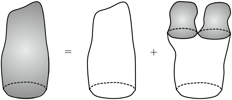
Figure 18: Graphical illustration of eq. (5). Shaded parts represent the generalized CDT disk amplitude, unshaded parts the original CDT disk amplitude and the original CDT propagator (5).

(2) Using eq. (128) we can expand $w(z)$ into a power series in $G_{s}/(2\Lambda_{{\rm cdt}})^{3/2}$ whose radius of convergence is $1/3\sqrt{3}$. For fixed values of $\Lambda_{{\rm cdt}}$, this value corresponds to the largest value of $G_{s}$ where (128) has a positive solution for $h$. The existence of such a bound on $G_{s}$ for fixed $\Lambda_{{\rm cdt}}$ was already observed in alwz . This bound can be re-expressed more transparently in the present Euclidean context, where it is more natural to keep the “Euclidean” cosmological constant $\Lambda$ fixed, rather than $\Lambda_{{\rm cdt}}$. We have

$$\frac{G_{s}}{(2\Lambda_{{\rm cdt}})^{3/2}}\leq\frac{1}{3\sqrt{3}}~{}\Rightarrow~{}\frac{{3}G_{s}^{2/3}}{2\Lambda+{3}G_{s}^{2/3}}\leq 1,$$ (135)

which for fixed $\Lambda>0$ is obviously satisfied for all positive $G_{s}$. In order to see that the usual Euclidean 2d quantum gravity (characterized by some finite value for $g_{s}$) can be re-derived from the disk amplitude (127), let us expand eq. (127) for large $G_{s}$. The square root part becomes

$$a^{-1}\;G_{s}^{-5/6}\;\left(Z-\sqrt{2\Lambda/3}\right)\sqrt{Z+2\sqrt{2\Lambda/3}},$$ (136)

which coincides with the generic expression $a^{3/2}W(Z,\Lambda)$ in Euclidean 2d quantum gravity (c.f. eqs. (106) and (107)) if we take $G_{s}$ to infinity as $g_{s}/a^{3}$ (and take into account a trivial rescaling of the cosmological constant). However, if we reintroduce the same scaling in the $V^{\prime}(z)$-part of $w(z)$, it does not scale with $a$ but simply goes to a constant. This term would dominate $w(z)$ in the limit $a\to 0$ if one did not remove it by hand, as is usually done in the Euclidean model.

(3) Why does the potential $V^{\prime}(z)$ (and therefore the entire disk amplitude $w(z)$) scale (like $1/a$) in the new continuum limit with $g_{s}=G_{s}a^{3}$, $a\to 0$, contrary to the situation in ordinary Euclidean quantum gravity? This is most clearly seen by looking again at the definitions (123) and (125). Because of the vanishing

$$V^{\prime}({\bar{z}},{\bar{g}})=0,~{}~{}~{}~{}V^{\prime\prime}({\bar{z}},{\bar{g}})=0$$ (137)

in the point $({\bar{z}},{\bar{g}})=(1,1/2)$, expanding around $({\bar{z}},{\bar{g}})$ according to (123), (125) leads automatically to a potential which is of order $a^{2}$ when expressed in terms of the renormalized constants $(Z_{\rm cdt},\Lambda_{{\rm cdt}})$, precisely like the square-root term when expressed in terms of $(Z_{\rm cdt},\Lambda_{{\rm cdt}})$.

The point $({\bar{z}},{\bar{g}})$ differs from the critical point $(z_{c}(g_{s}),g_{c}(g_{s}))$, as long as $g_{s}\not=0$. In fact, both $1/{\bar{z}}$ and ${\bar{g}}$ lie beyond the radii of convergence of $1/z$ and $g$, which are precisely $1/z_{c}(g_{s})$ and $g_{c}(g_{s})$. However, since the differences are of order $a$ and $a^{2}$, respectively, they simply amount to shifts in the renormalized variables, as made explicit in eqs. (124) and (126). Therefore, re-expressing $W(Z,\Lambda,G_{s})$ in (129) in terms of the variables $Z_{\rm cdt}$ and $\Lambda_{{\rm cdt}}$ simply leads to the expression $W_{\rm cdt}(Z_{\rm cdt},\Lambda_{{\rm cdt}},G_{s})$, first derived in alwz . Similarly, any geometric quantities defined with respect to $Z$ and $\Lambda$ can equally well be expressed in terms of $Z_{\rm cdt}$ and $\Lambda_{{\rm cdt}}$. For instance, the average continuum length of the boundary and the average continuum area of a triangulation are given by

$$\langle L\rangle=\frac{\partial\ln W(Z,\Lambda,G_{s})}{\partial Z}=\frac{\partial\ln W_{\rm cdt}(Z_{\rm cdt},\Lambda_{{\rm cdt}},G_{s})}{\partial Z_{\rm cdt}},$$ (138)

$$\langle A\rangle=\frac{\partial\ln W(Z,\Lambda,G_{s})}{\partial\Lambda}=\frac{\partial\ln W_{\rm cdt}(Z_{\rm cdt},\Lambda_{{\rm cdt}},G_{s})}{\partial\Lambda_{{\rm cdt}}}.$$ (139)

In the limit of $G_{s}\to 0$, the variables $(Z,\Lambda)$ and $(Z_{\rm cdt},\Lambda_{{\rm cdt}})$ become identical and the disk amplitude becomes the original CDT amplitude $(Z_{\rm cdt}+\sqrt{2\Lambda_{{\rm cdt}}})^{-1}$ alluded to in (130).

6 Matrix model representation

Above we have solved the two-dimensional gravity models by purely combinatorial techniques which emphasize the geometric interpretation: the quantum theory as a sum over geometries. The use of so-called matrix models allows one to perform the summation over the piecewise linear geometries in a relatively simple way. Surprisingly, it turns out that the scaling limit of the generalized CDT model has itself a matrix model representation. We will here describe how matrix models can be used instead of the combinatorial methods and how one is led to the CDT matrix model.

Let $\phi$ be a Hermitian $N\times N$ matrix with matrix elements $\phi_{\alpha\beta}$ and consider for $k=0,1,2,\ldots$ the integral

$$\int d\phi\;e^{-\frac{1}{2}\mathrm{tr}\,\phi^{2}}\frac{1}{k!}\left(\frac{1}{3}\mathrm{tr}\,\phi^{3}\right)^{k},$$ (140)

where

$$d\phi=\prod_{\alpha\leq\beta}d\,{\rm Re}\,\phi_{\alpha\beta}\prod_{\alpha<\beta}d\,{\rm Im}\,\phi_{\alpha\beta}.$$ (141)

We can regard $\phi$ as a zero-dimensional matrix-valued field so the integral can be evaluated in the standard way by doing all possible Wick contractions of $(\mathrm{tr}\,\phi^{3})^{k}$ and using

$$\left\langle\phi_{\alpha\beta}\phi_{\alpha^{\prime}\beta^{\prime}}\right\rangle=C\int d\phi\;e^{-\frac{1}{2}\sum_{\alpha\beta}|\phi_{\alpha\beta}|^{2}}\phi_{\alpha\beta}\phi_{\alpha^{\prime}\beta^{\prime}}=\delta_{\alpha\beta^{\prime}}\delta_{\beta\alpha^{\prime}},$$ (142)

where $C$ is a normalization factor. The evaluation of the expression (140) can be interpreted graphically by associating to each factor $\mathrm{tr}\,\phi^{3}$ an oriented triangle and to each term $\phi_{\alpha\beta}\phi_{\beta\gamma}\phi_{\gamma\alpha}$ contributing to the trace a labeling of its vertices by $\alpha,\beta,\gamma$ in cyclic order, such that the matrix element $\phi_{\alpha\beta}$ is associated with the oriented link whose endpoints are labeled by $\alpha$ and $\beta$ in accordance with the orientation. eq. (142) can then be interpreted as a gluing of the link labeled by $(\alpha\beta)$ to an oppositely oriented copy of the same link, see Fig. 19.

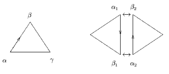
Figure 19: The matrix representation of triangles which converts the gluing along links to a Wick contraction.

In this way the integral (140) can be represented as a sum over closed, possibly disconnected, triangulations with $k$ triangles. Triangulations with an arbitrary genus arise in this representation. By summing over $k$ in (140) it follows by standard arguments that the (formal) logarithm of the corresponding integral is represented as a sum over all closed and connected triangulations. The contribution of a given triangulation can be determined by observing that in the process of gluing we pick up a factor of $N$ whenever a vertex becomes an internal vertex in the triangulation. Thus, the weight of a triangulation $T$ is simply

$$N^{N_{v}(T)}.$$

If we make the substitution

$$\mathrm{tr}\,\phi^{3}\to\frac{g}{\sqrt{N}}\mathrm{tr}\,\phi^{3},$$ (143)

the weight of $T$ is replaced by

$$g^{k}N^{N_{v}(T)-k/2}=g^{k}N^{\chi(T)},$$

where $\chi(T)$ is the Euler characteristic of $T$. Note also that the factor $(k!)^{-1}$ in (140) is cancelled in the sum over different triangulations because of the $k!$ possible permutations of the triangles, except for triangulations with non-trivial automorphisms, in which case the symmetry factor $C_{T}^{-1}$ survives. With the identifications

$$\frac{1}{G}=\log N,~{}~{}~{}~{}~{}\mu=-\log g$$ (144)

we conclude that

$$Z(\mu,G)=\log\frac{Z(g,N)}{Z(0,N)}$$ (145)

where $Z(\mu,\kappa)$ is defined by eq. (59)–(60) and

$$Z(g,N)=\int d\phi\;\exp\left(-\frac{1}{2}\mathrm{tr}\,\phi^{2}+\frac{g}{3\sqrt{N}}\mathrm{tr}\,\phi^{3}\right).$$ (146)

The integral (146) is of course divergent and should just be regarded as a shorthand for the formal power series in the coupling constant $g$.

It is straightforward to generalize the preceding arguments to the case of general unrestricted triangulations, where arbitrary polygons are allowed. Instead of one coupling constant $g$ we have a set $g_{1},g_{2},g_{3},\ldots$, but we will still use the notation $g$ or $g_{i}$. In this case eq. (146) is replaced by

$$Z(g_{i},N))=\int d\phi\;e^{-N\mathrm{tr}\,V(\phi)},$$ (147)

where the potential $V$, which depends on all the coupling constants $g_{i}$, is given by

$$V(\phi)=\frac{1}{2}\phi^{2}-\sum_{j=1}^{\infty}\frac{g_{j}}{j}\phi^{j}.$$ (148)

In eq. (148) we have scaled $\phi\to\sqrt{N}\phi$ for later convenience. It is not difficult to check that the obvious generalization of eq. (145) holds and the weight of a triangulation $T$ is given by

$$C_{T}^{-1}N^{\chi(T)}\prod_{j\geq 1}g_{j}^{N_{j}(T)},$$

where $N_{j}(T)$ is the number of $j$-gons in $T$. eq. (147) is of course a representation of a formal power series which is obtained by expanding the exponential of the non-quadratic terms as a power series in the coupling constants and then performing the Gaussian integrations term by term.

Differentiating $\log Z(g_{i},N)$ with respect to the coupling constants $g_{j}$, one obtains the expectation values of products of traces of powers of $\phi$. These expectation values have a straightforward interpretation in terms of triangulations. Denoting the expectation with respect to the measure

$$Z(g_{i},N)^{-1}e^{-N\mathrm{tr}\,V(\phi)}\,d\phi$$

by $\left\langle\cdot\right\rangle$ we see, for example, that $\left\langle N^{-1}\mathrm{tr}\,\phi^{n}\right\rangle$ is given by the sum over all connected triangulations of arbitrary genus whose boundary is an $n$-gon with one marked link. Similarly,

$$\frac{1}{N^{2}}\left\langle\mathrm{tr}\,\phi^{n}\mathrm{tr}\,\phi^{m}\right\rangle-\frac{1}{N^{2}}\left\langle\mathrm{tr}\,\phi^{n}\right\rangle\left\langle\mathrm{tr}\,\phi^{m}\right\rangle$$ (149)

is given by the sum over all connected triangulations whose boundary consists of two components with $n$ and $m$ links. More generally, the relation to the combinatorial problem is given by

$$w(g_{i},z_{1},\ldots,z_{b})=N^{b-2}\sum_{k_{1},\ldots,k_{b}}\frac{\left\langle\mathrm{tr}\,\phi^{k_{1}}\cdots\mathrm{tr}\,\phi^{k_{b}}\right\rangle_{conn}}{z^{k_{1}+1}_{1}\cdots z^{k_{b}+1}_{b}},$$ (150)

where the subscript conn indicates the connected part of the expectation $\left\langle\cdot\right\rangle$. One can rewrite eq. (150) as

$$w(g_{i},z_{1},\ldots,z_{b})=N^{b-2}\left\langle\mathrm{tr}\,\frac{1}{z_{1}-\phi}\;\cdots\;\mathrm{tr}\,\frac{1}{z_{b}-\phi}\right\rangle_{conn}.$$ (151)

The one-loop function $w(g_{i},z)$ is related to the density $\rho(\lambda)$ of eigenvalues of $\phi$ defined by

$$\rho(\lambda)=\left\langle\sum_{i=1}^{N}\delta(\lambda-\lambda_{i})\right\rangle,$$ (152)

where $\lambda_{i}$, $i=1,\ldots,N$ denote the $N$ eigenvalues of the matrix $\phi$. With this definition we have

$$\frac{1}{N}\left\langle\mathrm{tr}\,\phi^{n}\right\rangle=\int^{\infty}_{-\infty}d\lambda\;\rho(\lambda)\lambda^{n},~{}~{}~{}n\geq 0.$$ (153)

Hence,

$$w(g_{i},z)=\int_{-\infty}^{\infty}d\lambda\;\frac{\rho(\lambda)}{z-\lambda}.$$ (154)

In the limit $N\to\infty$ the support of $\rho$ is confined to a finite interval $[c_{-},c_{+}]$ on the real axis. In this case $w(z)$ will be an analytic function in the complex plane, except for a cut along the interval $[c_{-},c_{+}]$. Note that $\rho(\lambda)$ is determined from $w(z)$ by

$$2\pi i\rho(\lambda)=\lim_{\varepsilon\to 0}\left(w(\lambda-i\varepsilon)-w(\lambda+i\varepsilon)\right).$$ (155)

6.1 The loop equations

A standard method in quantum field theory is to derive identities by a change of variables in functional integrals. Here we apply this method to the matrix models and explore the invariance of the matrix integral (147) under infinitesimal field redefinitions of the form

$$\phi\to\phi+\varepsilon\phi^{n},$$ (156)

where $\varepsilon$ is an infinitesimal parameter. One can show that to first order in $\varepsilon$ the measure $d\phi$ defined by eq. (141) transforms as

$$d\phi\to d\phi\left(1+\varepsilon\sum_{k=0}^{n}\mathrm{tr}\,\phi^{k}\;\mathrm{tr}\,\phi^{n-k}\right).$$ (157)

The action transforms according to

$$\mathrm{tr}\,V(\phi)\to\mathrm{tr}\,V(\phi)+\varepsilon\mathrm{tr}\,\phi^{n}V^{\prime}(\phi)$$ (158)

to first order in $\varepsilon$. We can use these formulas to study the transformation of the measure under more general field redefinitions of the form

$$\phi\to\phi+\varepsilon\sum_{k=0}^{\infty}\frac{\phi^{k}}{z^{k+1}}=\phi+\varepsilon\frac{1}{z-\phi}.$$ (159)

This field redefinition only makes sense if $z$ is on the real axis outside the support $\rho$. In the limit $N\to\infty$ this is possible for $z$ outside the interval $[c_{-},c_{+}]$. Under the field redefinitions (159) the transformations of the measure and the action are given by

$$d\phi\to d\phi\left(1+\varepsilon\,\mathrm{tr}\,\frac{1}{z-\phi}\;\mathrm{tr}\,\frac{1}{z-\phi}\right),$$ (160)

$$\mathrm{tr}\,V(\phi)\to\mathrm{tr}\,V(\phi)+\varepsilon\,\mathrm{tr}\,\left(\frac{1}{z-\phi}V^{\prime}(\phi)\right).$$ (161)

The integral (147) is of course invariant under this change of the integration variables. By use of eqs. (160) and (161) we obtain the identity

$$\int d\phi\left\{\left(\mathrm{tr}\,\frac{1}{z-\phi}\right)^{2}-N\mathrm{tr}\,\left(\frac{1}{z-\phi}V^{\prime}(\phi)\right)\right\}\,e^{-N\mathrm{tr}\,V(\phi)}=0.$$ (162)

The contribution to the integral coming from the first term in $\{\cdot\}$ in eq. (162) is, by definition,

$$N^{2}w^{2}(z)+w(z,z).$$ (163)

The contribution from the second term inside $\{\cdot\}$ in eq. (162) can be written as an integral over the one-loop function as follows:

$$\frac{1}{N}\left\langle\mathrm{tr}\,\frac{V^{\prime}(\phi)}{z-\phi}\right\rangle=\int d\lambda\,\rho(\lambda)\,\frac{V^{\prime}(\lambda)}{z-\lambda}=\oint_{C}\frac{d\omega}{2\pi i}\,\frac{V^{\prime}(\omega)}{z-\omega}\;w(\omega),$$ (164)

where the second equality follows from eq. (155). The curve $C$ encloses the support of $\rho$ but not $z$. It is essential for the existence of $C$ that $\rho$ have compact support. We can then write eq. (162) in the form

$$\oint_{C}\frac{d\omega}{2\pi i}\frac{V^{\prime}(\omega)}{z-\omega}\;w(\omega)=w^{2}(z)+\frac{1}{N^{2}}w(z,z),$$ (165)

where $z$ is outside the interval $[c_{-},c_{+}]$ on the real axis. Since both sides of eq. (165) can be analytically continued to $C\setminus[c_{-},c_{+}]$ the equation holds in this domain.

We recognize eq. (165) as the loop equation already derived by combinatorial means, except that we here have an additional term involving $w(z,z)$ and with a coefficient $1/N^{2}$. In fact, (165) is the starting point for a $1/N^{2}$-expansion, i.e. a higher-genus expansion. To leading order in $1/N^{2}$ we have (as already derived)

$$w(z)=w_{0}(z)=\frac{1}{2}\left(V^{\prime}(z)-M(z)\sqrt{(z-c_{+})(z-c_{-})}\right)$$ (166)

and from eq. (155) the corresponding eigenvalue density is

$$\rho(\lambda)=\frac{1}{2\pi}M(\lambda)\sqrt{(c_{+}-\lambda)(\lambda-c_{-})}.$$ (167)

Let us now discuss how the new scaling limit is described in the matrix formalism. Hermitian matrix models are often analyzed in terms of the dynamics of their eigenvalues. Since the action in (147) is invariant under the transformation $\phi\to U\phi U^{\dagger}$, with $U\in U(N)$ a unitary $N\times N$-matrix, one can integrate out the “angular” degrees of freedom. What is left is an integration over the eigenvalues $\lambda_{i}$ of $\phi$ only,

$$Z(g)\propto\int\prod_{i=1}^{N}d\lambda_{i}\;e^{-N\sum_{j}V(\lambda_{j})}\;\prod_{k<l}|\lambda_{k}-\lambda_{l}|^{2},$$ (168)

where the last factor, the Vandermonde determinant, comes from integrating over the angular variables, and where

$${\rm tr}\ V(\phi)=\sum_{i=1}^{N}V(\lambda_{i}).$$ (169)

Naively one might expect that the large-$N$ limit is dominated by a saddle-point with $V^{\prime}(\lambda)=0$. However, this is not the case since the Vandermonde determinant in (168) contributes in the large-$N$ limit. The cut which appears in $w(z)$ is a direct result of the presence of the Vandermonde determinant. In this way one can say that the dynamics of the eigenvalues is “non-classical”, deviating from $V^{\prime}(\lambda)=0$, the size of the cut being a measure of this non-classicality. To get to the generalized CDT model we introduced a new coupling constant $g_{s}$ in the matrix model by substituting

$$V(\phi)\to\frac{1}{g_{s}}\;V(\phi),$$ (170)

and considered the limit $g_{s}\to 0$. As we have seen the coupling constant $g_{s}$ controls and reduces the size of the cut and thus brings the system closer to a “classical” behaviour. Thus the quantum fluctuations are reduced in the generalized CDT models.

Let us now consider the matrix potential (116), which formed the starting point of our new scaling analysis. We are still free to perform a change of variables. Inspired by relations (123)–(126), let us transform to new “CDT”-variables

$$\phi\to{\bar{z}}\,{\hat{I}}+a\Phi+O(a^{2}),$$ (171)

at the same time re-expressing $g$ as

$$g={\bar{g}}(1-a^{2}\Lambda_{{\rm cdt}}+O(a^{4})),$$ (172)

following eq. (123). Substituting the variable change into the matrix potential, and discarding a $\phi$-independent constant term, one obtains

$$V(\phi)={\bar{V}}(\Phi)\equiv\frac{\Lambda_{{\rm cdt}}\Phi-\frac{1}{6}\Phi^{3}}{2G_{s}}$$ (173)

in the limit $a\to 0$, from which it follows that

$$Z(g,g_{s})=a^{N^{2}}Z(\Lambda_{{\rm cdt}},G_{s}),~{}~{}~{}Z(\Lambda_{{\rm cdt}},G_{s})=\int d\Phi\;\mbox{e}^{-N\mathrm{tr}\,{\bar{V}}(\Phi)}.$$ (174)

The disk amplitude for the potential ${\bar{V}}(\Phi)$ is precisely $W(Z_{\rm cdt},\Lambda_{{\rm cdt}},G_{s})$, and since by definition

$$\frac{1}{z-\phi}=\frac{1}{a}\,\frac{1}{Z_{\rm cdt}-\Phi},$$ (175)

the first equal sign in eq. (129) follows straightforwardly from the simple algebraic equation (173). We conclude that the continuum generalized CDT-theory is described by the matrix model with potential ${\bar{V}}(\Phi)$.

The conclusion is that to leading order in $N$, the combinatorial method which works with a regularized lattice theory with a geometric interpretation and an explicit cut-off $a$ has a matrix model representation, and even in the continuum limit where $a\to 0$ there exists a matrix model representation of the theory. Once this is proved, one can actually “derive” a number of the results known for the generalized CDT model from the matrix model by the formal manipulations of eqs. (173)-(174), where $a$ appears merely as a parameter without any obvious geometric interpretation as a cut-off. Also, once the matrix model equivalence is established, it is clear that one has automatically a higher-genus expansion available. This higher-genus expansion was first established working with the combinatorial, generalized CDT theory, and based on purely geometric arguments of splitting and joining of space as a function of proper time, as we (partly) described above. Such a theory could be turned into a kind of string field theory, imitating the work of Kawai and collaborators on Euclidean quantum gravity sft . Like in the Euclidean case of Kawai et al., the formulation of the CDT string field theory used entirely a continuum notation (i.e. to cut-off $a$ was already taken to zero). However, contrary to the situation for the Euclidean string field theory, we now have a matrix model representation even in the continuum, and many of the string field theory results derived in alwz follow easily from the loop equations (165) for the potential (173).

6.2 Summation over all genera in the CDT matrix model

One remarkable application of the CDT matrix model representation is that we can find the Hartle-Hawking wave function summed over all genera.

In alwz the matrix model given by eqs. (173) and (174) was related to the CDT Dyson-Schwinger equations by (i) introducing into the latter an expansion parameter $\alpha$, which kept track of the genus of the two-dimensional spacetime, and (ii) identifying this parameter with $1/N^{2}$, where $N$ is the size of the matrix in the matrix integral. The $1/N$-expansion of our matrix model therefore plays a role similar to the $1/N$-expansion originally introduced by ’t Hooft: it reorganizes an asymptotic expansion in a coupling constant $t$ ($t=G_{s}/(\sqrt{\Lambda_{{\rm cdt}}})^{3/2}$ in our case) into convergent sub-summations in which the $k$th summand appears with a coefficient $N^{-2k}$. In QCD applications, the physically relevant value is $N=3$, to which the leading-order terms in the large $N$-expansion can under favourable circumstances give a reasonable approximation.

As we will see, for the purposes of solving our string field-theoretic model non-perturbatively, an additional expansion in inverse powers of $N$ (and thus an identification of the contributions at each particular genus) is neither essential nor does it provide any new insights. This means that we will consider the entire sum over topologies “in one go”, which simply amounts to setting $N=1$, upon which the matrix integral (174) reduces to the ordinary integral

$$Z(G_{s},\Lambda_{{\rm cdt}})=\int\mbox{d}m\;\exp\left[-\frac{1}{2G_{s}}\left(\Lambda_{{\rm cdt}}m-\frac{1}{6}\;m^{3}\right)\right],$$ (178)

while the disk amplitude can be written as

$$W_{\rm cdt}(X)=\frac{1}{Z(G_{s},\Lambda_{{\rm cdt}})}\int\mbox{d}m\;\frac{\exp\left[-\frac{1}{2G_{s}}\left(\Lambda_{{\rm cdt}}m-\frac{1}{6}\;m^{3}\right)\right]}{X-m}.$$ (179)

These integrals should be understood as formal power series in the dimensionless variable $t=G_{s}/(\sqrt{\Lambda_{{\rm cdt}}})^{3/2}$ appearing in eq. (128). Any choice of an integration contour which makes the integral well defined and reproduces the formal power series is a potential non-perturbative definition. However, different contours might produce different non-perturbative contributions (i.e. which cannot be expanded in powers of $t$), and there may even be non-perturbative contributions which are not captured by any choice of integration contour. As usual in such situations, additional physics input is needed to fix these contributions.

To illustrate the point, let us start by evaluating the partition function given in (178). We have to decide on an integration path in the complex plane in order to define the integral. One possibility is to take a path along the negative axis and then along either the positive or the negative imaginary axis. The corresponding integrals are

$$Z(g,\lambda)=\sqrt{\Lambda_{{\rm cdt}}}\;t^{1/3}F_{\pm}(t^{-2/3}),~{}~{}~{}F_{\pm}(t^{-2/3})=2\pi\;e^{\pm i\pi/6}{\rm Ai}(t^{-2/3}\mbox{e}^{\pm 2\pi i/3}),$$ (180)

where Ai denotes the Airy function. Both $F_{\pm}$ have the same asymptotic expansion in $t$, with positive coefficients. Had we chosen the integration path entirely along the imaginary axis we would have obtained ($2\pi i$ times) ${\rm Ai}(t^{-2/3})$, but this has an asymptotic expansion in $t$ with coefficients of oscillating sign, which is at odds with its explicit power expansion in $t$. We have (using the standard notation of Airy functions)

$$F_{\pm}(z)=\pi\Big{(}{\rm Bi}(z)\pm i{\rm Ai}(z)\Big{)},$$ (181)

from which one deduces immediately that the functions $F_{\pm}(t^{-2/3})$ are not real. However, since ${\rm Bi}(t^{-2/3})$ grows like $e^{\frac{2}{3t}}$ for small $t$ while ${\rm Ai}(t^{-2/3})$ falls off like $e^{-\frac{2}{3t}}$, their imaginary parts are exponentially small in $1/t$ compared to the real part, and therefore do not contribute to the asymptotic expansion in $t$. An obvious way to define a partition function which is real and shares the same asymptotic expansion is by symmetrization,

$$\frac{1}{2}(F_{+}+F_{-})\equiv\pi{\rm Bi}.$$ (182)

The situation parallels the one encountered in the double-scaling limit of the “old” matrix model but is less complicated.

Presently, let us collectively denote by $F(z)$ any of the functions $F_{\pm}(z)$ or $\pi{\rm Bi}(z)$, leading to the tentative identification

$$Z(G_{s},\Lambda_{{\rm cdt}})=\sqrt{\Lambda_{{\rm cdt}}}\;t^{1/3}\,F\Big{(}t^{-2/3}\Big{)},~{}~{}~{}~{}F^{\prime\prime}(z)=zF(z),$$ (183)

where we have included the differential equation satisfied by the Airy functions for later reference. Assuming $X>0$, we can write

$$\frac{1}{X-m}=\int_{0}^{\infty}\mbox{d}L\;\exp\left[-\left(X-m\right)L\right].$$ (184)

We can use this identity in eq. (179) to obtain the integral representation

$$W_{\rm cdt}(X)=\int_{0}^{\infty}\mbox{d}L\;\mbox{e}^{-XL}\;\frac{F\Big{(}t^{-2/3}-t^{1/3}\sqrt{\Lambda_{{\rm cdt}}}L\Big{)}}{F\Big{(}t^{-2/3}\Big{)}}.$$ (185)

From the explicit expression of the Laplace transform we can now read off the Hartle-Hawking amplitude as function of the boundary length $L$,

$$W_{\rm cdt}(L)=\frac{F(t^{-2/3}-t^{1/3}\sqrt{\Lambda_{{\rm cdt}}}\,L)}{F(t^{-2/3})}.$$ (186)

Before turning to a discussion of the non-perturbative expression for $W_{\rm cdt}(L)$ we have just derived, let us remark that the asymptotic expansion in $t$ of course agrees with that obtained by recursively solving the CDT Dyson-Schwinger equations. Using the standard asymptotic expansion of the Airy function one obtains

$$W_{\rm cdt}(L)=\mbox{e}^{-\sqrt{\Lambda_{{\rm cdt}}}\,L}\;\mbox{e}^{t\,h(t,\sqrt{\Lambda_{{\rm cdt}}}\,L)}\;\;\frac{\sum_{k=0}^{\infty}c_{k}\;t^{k}\;(1-t\sqrt{\Lambda_{{\rm cdt}}}\,L)^{-\frac{3}{2}k-\frac{1}{4}}}{\sum_{k=0}^{\infty}c_{k}\;t^{k}},$$ (187)

where the coefficients $c_{k}$ are given by $c_{0}=1$, $c_{k}=\frac{1}{k!}\left(\frac{3}{4}\right)^{k}\left(\frac{1}{6}\right)_{k}\left(\frac{5}{6}\right)_{k}$, $k>0$. In (187), we have rearranged the exponential factors to exhibit the exponential fall-off in the length variable $L$, multiplied by a term containing the function

$$h(t,\sqrt{\Lambda_{{\rm cdt}}}\,L)=\frac{2}{3t^{2}}\left[(1-t\sqrt{\Lambda_{{\rm cdt}}}\,L)^{3/2}-1+\frac{3}{2}t\sqrt{\Lambda_{{\rm cdt}}}\,L\right],$$ (188)

which has an expansion in positive powers of $t$.

$W_{\rm cdt}(L)$ has the interpretation of the wave function of the spatial universe according to the hypothesis of Hartle and Hawking. $L\in[0,\infty]$ and the probability of finding a spatial universe with length between $L$ and $L+\mbox{d}L$ is

$$P(L)=\frac{|W_{\rm cdt}(L)|^{2}}{L},$$ (189)

since the integration measure is $\mbox{d}L/L$. Thus the probability is not normalizable in a conventional way and peaked at $L=0$ since $W_{\rm cdt}(L=0)=1$. However, for each term in the asymptotic expansion (187) we obtain a finite value $\langle L\rangle\sim 1/\sqrt{\Lambda_{{\rm cdt}}}$ as one would naturally expect. Since termination of the series in (187) at a finite $k$ also implies restricting the 2d spacetime to have a finite genus we can say that as long as we restrict spacetime to have finite genus we have $\langle L\rangle\sim 1/\sqrt{\Lambda_{{\rm cdt}}}$. However, if we allow spacetimes of arbitrarily large genus to appear, i.e. if topology fluctuations are unconstrained (that means at most suppressed by a coupling constant, but no upper limit on the genus imposed by hand), a remarkable change appears: $\langle L\rangle=\infty$ because the full non-perturbative $W_{\rm cdt}(L)$ does not fall off like $\mbox{e}^{-\sqrt{\Lambda_{{\rm cdt}}}\;L}$ but only as $L^{-1/4}$ (Note that $W_{\rm cdt}(L)$ is still integrable at infinity since the integration measure is $\mbox{d}L/L$). This dramatic change in large $L$ behaviour ($W(L)$ also becomes oscillatory for large $L$, despite the fact that each term in the asymptotic expansion (187) is positive) is clearly to be attributed to surfaces of arbitrarily large genus, i.e. it is a genuinely non-perturbative result.

7 Discussion and perspectives

The four-dimensional CDT model of quantum gravity is extremely simple. It is the path integral over the class of causal geometries with a global time foliation. In order to perform the summation explicitly, we introduce a grid of piecewise linear geometries, much in the same way as when defining the path integral in quantum mechanics. Next, we rotate each of these geometries to Euclidean signature and use as bare action the Einstein-Hilbert action in Regge form. That is all.

The resulting superposition exhibits a nontrivial scaling behaviour as function of the four-volume, and we observe the appearance of a well-defined average geometry, that of de Sitter space, the maximally symmetric solution to the classical Einstein equations in the presence of a positive cosmological constant. We are definitely in a quantum regime, since the fluctuations of the three-volume around de Sitter space are sizable, as can be seen in Fig. 7. Both the average geometry and the quantum fluctuations are well described in terms of the minisuperspace action (25). A key feature to appreciate is that, unlike in standard (quantum-)cosmological treatments, this description is the outcome of a non-perturbative evaluation of the full path integral, with everything but the scale factor (equivalently, $V_{3}(t)$) summed over. Measuring the correlations of the quantum fluctuations in the computer simulations for a particular choice of bare coupling constants enabled us to determine the continuum gravitational coupling constant $G$ as $G\approx 0.42a^{2}$, thereby introducing an absolute physical length scale into the dimensionless lattice setting. Within measuring accuracy, our de Sitter universes (with volumes lying in the range of 6.000-47.000 $\ell_{Pl}^{4}$) are seen to behave perfectly semi-classically with regard to their large-scale properties.

We have also indicated how we may be able to penetrate into the sub-Planckian regime by suitably changing the bare coupling constants. By “sub-Planckian regime” we mean that the lattice spacing $a$ is (much) smaller than the Planck length. While we have not yet analyzed this region in detail, we expect to eventually observe a breakdown of the semi-classical approximation. This will hopefully allow us to make contact with continuum attempts to define a theory of quantum gravity based on quantum field theory. One such attempt has been described in the introduction and is based on the concept of asymptotic safety. It uses renormalization group techniques in the continuum to study scaling violations in quantum gravity around a UV fixed point reuteretc . Other recent continuum field theoretical models of quantum gravity which are not in disagreement with our data are the so-called Lifshitz gravity model horava and the so-called scale-invariant gravity model shaposh1 ; shaposh2 . In principle it is only a question of computer power to decide if any of the models agree with our CDT model of quantum gravity.

On the basis of these results two major issues suggest themselves for further research. First, we need to establish the relation of our effective gravitational coupling constant $G$ with a more conventional gravitational coupling constant, defined directly in terms of coupling matter to gravity. In the present work, we have defined $G$ as the coupling constant in front of the effective action, but it would be desirable to verify directly that a gravitational coupling defined via the coupling to matter agrees with our $G$. In principle it is easy to couple matter to our model, but it is less straightforward to define in a simple way a set-up for extracting the semi-classical effect of gravity on the matter sector. Attempts in this direction were already undertaken in the “old” Euclidean approach js ; newton , and it is possible that similar ideas can be used in CDT quantum gravity.

The second issue concerns the precise nature of the “continuum limit”. Recall our discussion in the Introduction about this in a conventional lattice-theoretic setting. The continuum limit is usually linked to a divergent correlation length at a critical point. It is unclear whether such a scenario is realized in our case. In general, it is rather unclear how one could define at all the concept of a divergent length related to correlators in quantum gravity, since one is integrating over all geometries, and it is the geometries which dynamically give rise to the notion of “length”.

This has been studied in detail in two-dimensional (Euclidean) quantum gravity coupled to matter with central charge $c\leq 1$ corr2d . It led to the conclusion that one could associate the critical behaviour of the matter fields (i.e. approaching the critical point of the Ising model) with a divergent correlation length, although the matter correlators themselves had to be defined as non-local objects due to the requirement of diffeomorphism invariance. On the other hand, the two-dimensional studies do not give us a clue of how to treat the gravitational sector itself, since they do not possess gravitational field-theoretic degrees of freedom. As we have seen the two-dimensional lattice models can be solved analytically and the only fine-tuning needed to approach the continuum limit is an additive renormalization of the cosmological constant. Thus, fixing the two-dimensional spacetime volume $N_{2}$ (the number of triangles), such that the cosmological constant plays no role, there are no further coupling constants to adjust and the continuum limit is automatically obtained by the assignment $V_{2}=N_{2}a^{2}$ and taking $N_{2}\to\infty$. This situation can also occur in special circumstances in ordinary lattice field theory. A term like

$$\sum_{i}c_{1}(\phi_{i+1}-\phi_{i})^{2}+c_{2}(\phi_{i+1}+\phi_{i-1}-2\phi_{i})^{2}$$ (190)

(or a higher-dimensional generalization) will also go to the continuum free field theory simply by increasing the lattice size and using the identification $V_{d}=L^{d}a^{d}$ ($L$ denoting the linear size of the lattice in lattice units), the higher-derivative term being sub-dominant in the limit. It is not obvious that in quantum gravity one can obtain a continuum quantum field theory without fine-tuning in a similar way, because the action in this case is multiplied by a dimensionful coupling constant. Nevertheless, it is certainly remarkable that the infrared limit of our effective action apparently reproduces – within the cosmological setting – the Einstein-Hilbert action, which is the unique diffeomorphism-invariant generalization of the ordinary kinetic term, containing at most second derivatives of the metric. A major question is whether and how far our theory can be pushed towards an ultraviolet limit. We have indicated how to obtain such a limit by varying the bare coupling constants of the theory, but the investigation of the limit $a\to 0$ with fixed $G$ has only just begun and other scenarios than a conventional UV fixed point might be possible. One scenario, which has often been discussed as a possibility, but which is still missing an explicit implementation is the following: when one approaches sub-Planckian scales the theory effectively becomes a topological quantum field theory where the metric plays no role. Also in our very explicit implementation of a quantum gravity model it is unclear how such a scenario would look.

Acknowledgments

The material presented in this review is based on collaborations with numerous colleagues. In particular, we would like to thank Andrzej Görlich, Willem Westra and Stefan Zohren who have contributed in an essential way to the more recent part of the material presented. All authors acknowledge support by ENRAGE (European Network on Random Geometry), a Marie Curie Research Training Network, contract MRTN-CT-2004-005616, and JJ by COCOS (Correlations in Complex Systems), a Marie Curie Transfer of Knowledge Project, contract MTKD-CT-2004-517186, both in the European Community’s Sixth Framework Programme. RL acknowledges support by the Netherlands Organisation for Scientific Research (NWO) under their VICI program. JJ acknowledges a partial support by the Polish Ministry of Science and Information Technologies grant 1P03B04029 (2005-2008).

References

- (1) S. Weinberg: Ultraviolet divergences in quantum theories of gravitation, in General relativity: Einstein centenary survey, eds. S.W. Hawking and W. Israel, Cambridge University Press, Cambridge, UK (1979) pp 790-831.
-
(2)
A. Codello, R. Percacci and C. Rahmede:
Investigating the ultraviolet properties of gravity with a Wilsonian
renormalization group equation,
Annals Phys. 324 (2009) 414-469,
[arXiv:0805.2909,[hep-th]];
M. Reuter and F. Saueressig: Functional renormalization group equations, asymptotic safety, and Quantum Einstein Gravity, Lectures given at First Quantum Geometry and Quantum Gravity School, Zakopane, Poland, 23 Mar - 3 Apr 2007. 57 pages [arXiv:0708.1317, hep-th];
M. Niedermaier and M. Reuter: The asymptotic safety scenario in quantum gravity, Living Rev. Rel. 9 (2006) 5; 173 pages;
H.W. Hamber and R.M. Williams: Nonlocal effective gravitational field equations and the running of Newton’s G, Phys. Rev. D 72 (2005) 044026, 16 pages [arXiv:hep-th/0507017];
D.F. Litim: Fixed points of quantum gravity, Phys. Rev. Lett. 92 (2004) 201301, 4 pages [arXiv:hep-th/0312114];
H. Kawai, Y. Kitazawa and M. Ninomiya: Renormalizability of quantum gravity near two dimensions, Nucl. Phys. B 467 (1996) 313-331 [arXiv:hep-th/9511217]. -
(3)
P. Hořava,
Spectral dimension of the universe in quantum gravity at a Lifshitz
point, 11 pages [arXiv:0902.3657 [hep-th]];
Quantum gravity at a Lifshitz point,, Phys. Rev. D 79 (2009) 084008, 15 pages [arXiv:0901.3775 [hep-th]]. -
(4)
M. Shaposhnikov and D. Zenhausern,
Quantum scale invariance, cosmological constant and hierarchy problem,
Phys. Lett. B 671 (2009) 162-166
[arXiv:0809.3406 [hep-th]];
Scale invariance, unimodular gravity and dark energy, Phys. Lett. B 671 (2009) 187-192 [arXiv:0809.3395 [hep-th]]. - (5) M.E. Shaposhnikov and I.I. Tkachev, Quantum scale invariance on the lattice, 5 pages [arXiv:0811.1967 [hep-th]].
- (6) J. Ambjørn, J. Jurkiewicz and R. Loll: Dynamically triangulating Lorentzian quantum gravity, Nucl. Phys. B 610 (2001) 347-382 [arXiv:hep-th/0105267].
- (7) Link to animation of 2d Lorentzian quantum gravity: http://www.nbi.dk/ ambjorn/lqg2/
- (8) J. Ambjørn, J. Jurkiewicz and R. Loll: Reconstructing the universe, Phys. Rev. D 72 (2005) 064014, 24 pages [arXiv:hep-th/0505154].
- (9) P. Bialas, Z. Burda, A. Krzywicki and B. Petersson: Focusing on the fixed point of 4d simplicial gravity, Nucl. Phys. B 472 (1996) 293-308 [arXiv:hep-lat/9601024].
- (10) J. Ambjørn and R. Loll: Non-perturbative Lorentzian quantum gravity, causality and topology change, Nucl. Phys. B 536 (1998) 407-434 [arXiv:hep-th/9805108].
- (11) J. Ambjørn, J. Jurkiewicz and R. Loll: Emergence of a 4D world from causal quantum gravity, Phys. Rev. Lett. 93 (2004) 131301, 4 pages [arXiv:hep-th/0404156].
- (12) J. Ambjørn, J. Jurkiewicz and R. Loll: Semiclassical universe from first principles, Phys. Lett. B 607 (2005) 205-213 [arXiv:hep-th/0411152].
- (13) J. Ambjørn, A. Görlich, J. Jurkiewicz and R. Loll: Planckian birth of the quantum de Sitter universe, Phys. Rev. Lett. 100 (2008) 091304, 4 pages [arXiv:0712.2485, [hep-th]].
- (14) J. Ambjørn, A. Görlich, J. Jurkiewicz and R. Loll: The nonperturbative quantum de Sitter universe, Phys. Rev. D 78 (2008) 063544, 17 pages [arXiv:0807.4481 [hep-th]].
-
(15)
J. Ambjørn, J. Jurkiewicz and R. Loll:
The universe from scratch,
Contemp. Phys. 47 (2006) 103-117 [arXiv:hep-th/0509010];
R. Loll: The emergence of spacetime, or, quantum gravity on your desktop, Class. Quant. Grav. 25 (2008) 114006, 17 pages [arXiv:0711.0273, [gr-qc]];
J. Ambjørn, A. Gorlich, J. Jurkiewicz and R. Loll: The quantum universe, Acta Phys. Polon. B 39 (2008) 3309-3341. -
(16)
C. Teitelboim:
Causality versus gauge invariance in quantum gravity and supergravity,
Phys. Rev. Lett. 50 (1983) 705-708;
The proper time gauge in quantum theory of gravitation, Phys. Rev. D 28 (1983) 297-309. -
(17)
J. Ambjørn, R. Loll, W. Westra and S. Zohren:
Putting a cap on causality violations in CDT,
JHEP 0712 (2007) 017, 16 pages [arXiv:0709.2784, [gr-qc]];
J. Ambjørn, R. Loll, Y. Watabiki, W. Westra and S. Zohren: A string field theory based on causal dynamical triangulations, JHEP 0805 (2008) 032, 26 pages [arXiv:0802.0719, [hep-th]];
A matrix model for 2D quantum gravity defined by causal dynamical triangulations, Phys. Lett. B 665 (2008) 252-256 [arXiv:0804.0252, [hep-th]];
A new continuum limit of matrix models, Phys. Lett. B 670 (2008) 224-230 [arXiv:0810.2408 [hep-th]];
A Causal Alternative for c=0 Strings, Acta Phys. Polon. B 39 (2008) 3355-3364 [arXiv:0810.2503 [hep-th]];
J. Ambjørn, R. Loll, W. Westra and S. Zohren: Summing over all Topologies in CDT String Field Theory,, 15 pages, arXiv:0905.2108 [hep-th]. -
(18)
J. Ambjørn, J. Jurkiewicz, R. Loll and G. Vernizzi:
Lorentzian 3d gravity with wormholes via matrix models,
JHEP 0109 (2001) 022, 34 pages [arXiv:hep-th/0106082];
3D Lorentzian quantum gravity from the asymmetric ABAB matrix model, Acta Phys. Polon. B 34 (2003) 4667-4688 [arXiv:hep-th/0311072];
J. Ambjørn, J. Jurkiewicz and R. Loll: Renormalization of 3d quantum gravity from matrix models, Phys. Lett. B 581 (2004) 255-262 [arXiv:hep-th/0307263]. - (19) D. Benedetti, R. Loll and F. Zamponi: (2+1)-dimensional quantum gravity as the continuum limit of causal dynamical triangulations, Phys. Rev. D 76 (2007) 104022, 26 pages [arXiv:0704.3214, [hep-th]].
-
(20)
J. Ambjørn, B. Durhuus and J. Fröhlich:
Diseases of triangulated random surface models, and possible cures,
Nucl. Phys. B 257 (1985) 433-449;
J. Ambjørn, B. Durhuus, J. Fröhlich and P. Orland: The appearance of critical dimensions in regulated string theories, Nucl. Phys. B 270 (1986) 457-482. - (21) A. Billoire and F. David: Microcanonical simulations of randomly triangulated planar random surfaces, Phys. Lett. B 168 (1986) 279-283.
- (22) D.V. Boulatov, V.A. Kazakov, I.K. Kostov and A.A. Migdal: Analytical and numerical study of the model of dynamically triangulated random surfaces, Nucl. Phys. B 275 (1986) 641-686.
-
(23)
J. Ambjørn and J. Jurkiewicz:
Four-dimensional simplicial quantum gravity,
Phys. Lett. B 278 (1992) 42-50;
Scaling in four-dimensional quantum gravity, Nucl. Phys. B 451 (1995) 643-676 [arXiv:hep-th/9503006]. - (24) M.E. Agishtein and A.A. Migdal, Simulations of four-dimensional simplicial quantum gravity, Mod. Phys. Lett. A 7 (1992) 1039-1062.
- (25) J. Ambjørn, J. Jurkiewicz and R. Loll: Spectral dimension of the universe, Phys. Rev. Lett. 95 (2005) 171301, 4 pages [arXiv:hep-th/0505113].
- (26) B. Dittrich and R. Loll: Counting a black hole in Lorentzian product triangulations, Class. Quant. Grav. 23 (2006) 3849-3878 [arXiv:gr-qc/0506035].
-
(27)
J. Ambjørn, S. Jain and G. Thorleifsson,
Baby universes in 2-d quantum gravity,
Phys. Lett. B 307 (1993) 34-39,
[arXiv:hep-th/9303149];
J. Ambjørn, S. Jain, J. Jurkiewicz and C. F. Kristjansen, Observing 4-d baby universes in quantum gravity, Phys. Lett. B 305 (1993) 208-213 [arXiv:hep-th/9303041]. - (28) J. Ambjørn and B. Durhuus, Regularized bosonic strings need extrinsic curvature,, Phys. Lett. B 188 (1987) 253-257.
- (29) B.V. de Bakker and J. Smit: Gravitational binding in 4D dynamical triangulation, Nucl. Phys. B 484 (1997) 476-494 [arXiv:hep-lat/9604023].
- (30) H.W. Hamber and R.M. Williams: Newtonian potential in quantum Regge gravity, Nucl. Phys. B 435 (1995) 361-398 [arXiv:hep-th/9406163].
-
(31)
J. Ambjørn, K.N. Anagnostopoulos, U. Magnea and G. Thorleifsson:
Geometrical interpretation of the KPZ exponents,
Phys. Lett. B 388 (1996) 713-719 [arXiv:hep-lat/9606012];
J. Ambjørn and K.N. Anagnostopoulos: Quantum geometry of 2D gravity coupled to unitary matter, Nucl. Phys. B 497 (1997) 445-478 [arXiv:hep-lat/9701006];
J. Ambjørn, K.N. Anagnostopoulos and R. Loll: A new perspective on matter coupling in 2d quantum gravity, Phys. Rev. D 60 (1999) 104035, 11 pages [arXiv:hep-th/9904012]. - (32) J. Ambjørn, J. Jurkiewicz and Yu.M. Makeenko, Multiloop correlators for two-dimensional quantum gravity, Phys. Lett. B 251 (1990) 517-524.
-
(33)
H. Kawai, N. Kawamoto, T. Mogami and Y. Watabiki,
Transfer matrix formalism for two-dimensional quantum gravity and fractal
structures of space-time,
Phys. Lett. B 306 (1993) 19-26
[arXiv:hep-th/9302133];
J. Ambjørn and Y. Watabiki, Scaling in quantum gravity, Nucl. Phys. B 445 (1995) 129-144 [arXiv:hep-th/9501049];
S. Catterall, G. Thorleifsson, M.J. Bowick and V. John, Scaling and the fractal geometry of two-dimensional quantum gravity, Phys. Lett. B 354 (1995) 58-68 [arXiv:hep-lat/9504009];
J. Ambjørn, J. Jurkiewicz and Y. Watabiki, On the fractal structure of two-dimensional quantum gravity, Nucl. Phys. B 454 (1995) 313-342 [arXiv:hep-lat/9507014];
H. Aoki, H. Kawai, J. Nishimura and A. Tsuchiya, Operator product expansion in two-dimensional quantum gravity, Nucl. Phys. B 474 (1996) 512-528 [arXiv:hep-th/9511117]. -
(34)
N. Ishibashi and H. Kawai,
String field theory of noncritical strings,
Phys. Lett. B 314 (1993) 190-196
[arXiv:hep-th/9307045];
String field theory of noncritical strings, Phys. Lett. B 322 (1994) 67-78 [arXiv:hep-th/9312047];
A Background independent formulation of noncritical string theory, Phys. Lett. B 352 (1995) 75-82 [arXiv:hep-th/9503134];
Y. Watabiki, Construction of noncritical string field theory by transfer matrix formalism in dynamical triangulation, Nucl. Phys. B 441 (1995) 119-156 [arXiv:hep-th/9401096];
M. Ikehara, N. Ishibashi, H. Kawai, T. Mogami, R. Nakayama and N. Sasakura,
String field theory in the temporal gauge, Phys. Rev. D 50 (1994) 7467-7478 [arXiv:hep-th/9406207];
A note on string field theory in the temporal gauge, Prog. Theor. Phys. Suppl. 118 (1995) 241-258 [arXiv:hep-th/9409101];
J. Ambjørn and Y. Watabiki, Non-critical string field theory for 2d quantum gravity coupled to (p,q)–conformal fields, Int. J. Mod. Phys. A 12 (1997) 4257-4289 [arXiv:hep-th/9604067].
Index
- asymptotic freedom §1, §4.4
- asymptotic safety §1, §3.3, §7
- background geometry §1, §3.1, §3.1, §3.2
- background-independent §1
- branched polymers Figure 12, §2, §2, §3.3, §3.3, §4.3, §4.3, §4.4
- causal dynamical triangulation: see CDT §1
- CDT §1, §1, §2, §3.1, §3.1, §3.3, §4.2, §5, §5, §5, §5, §6, §6.1, §6.1, §7
- CDT matrix model §6, §6.2
- CDT path integral §2, §2, §5, §7
- continuum limit §1, §2, §2, §4.2, §4.4, §4.4, §4.4, §5, §6.1, §7, §7
- correlation function §1, §3.2, §3.2, §3.2, §4.4, §7
- correlation length §1, §7, §7
- crumpled phase §2
- de Sitter universe §1, §3.1, §3.1, §3.2, §3.3, §7
- disk amplitude Figure 18, §5, §5, §5, §5, §5, §5, §5, §5, §5, §6.1, §6.1, §6.1, §6.1, §6.2
- double-scaling limit §4.4, §6.2
- eigenvalue density §6.1
- Einstein-Hilbert action §1, §2, §3.1, §4.1, §4.1, §7, §7
- emergent universe §3.1, §3.2
- Euclidean quantum gravity §1, §2, §2, §2, §2, §3.3, §4, §4.1, §4.4, §4.4, §5, §5, §5, §5, §5, §6.1, §7
- Euclidean signature §2, §2, §5
- generalized CDT model §5
- Hartle-Hawking wave function §4.2, §5, §6.2, §6.2, §6.2
- Hartle-Hawking wavefunction §4.1
- Hausdorff dimension §2
- Landau pole §1
- large expansion §6.2
- lattice regularization §1, §1, §4.2
- Lifshitz gravity §1
- loop correlator §4.2, §4.2, §4.3, §4.3, §4.4, §4.4, §6, §6.1
- loop equation §4.2, §6.1, §6.1, §6.1
- loop insertion operator §4.3, §4.3, §4.4
- loop quantum gravity §1
- Lorentzian path integral §2
- Lorentzian quantum gravity §1, §5
- Lorentzian signature footnote 1, §2, §5
- matrix model §4.2, §6, §6, §6.1, §6.1, §6.1, §6.1, §6.2
- Monte Carlo simulations §2, §2, §2, §2, §3, §3.2
- non-perturbative §1, §1, §1, §1, §2, §2, §3.3, §7
- non-renormalizable §1, §1
- path integral §1, §1, §2, §2, §2, §2
- perturbation theory §1, §1
- phase transition §1, §2, §2, §3.1, §3.3, §3.3
- piecewise linear geometries §1, §1, §2, §2, §2, §3.1, §6, §7
- Planck length §3.3, §3.3, §3.3, §3.3, §7
- quantum chromodynamics §1
- quantum field theory §1
- quantum fluctuations Figure 7, §1, §3, §3, §3.1, §3.1, §3.2, §3.3, §6.1, §7
- Regge action §2, §7
- renormalization group §1, §1
- scale-invariant gravity §1
- spacetime history §1, §2, §3
- string theory §1, §1
- sum over geometries §1, §2, §6, §6
- sum-over-histories §1, §1, §2
- ultraviolet fixed point Figure 1, §1, §1, §1, §1, §1, §1, §7, §7
- -function §1, §1, §4.4