On Coherence Lengths of Wave Packets

Abstract

The coherence lengths of one-particle states described using quantum wave functions are studied. We show that one particle states in various situations are not described using simple plane waves but using wave packets that are superpositions of plane waves. A wave packet is an approximate eigenstate of the free Hamiltonian and has a finite spatial size that we call the coherence length. The coherence lengths in the coordinate space and momentum space are studied in this paper. We investigate several mechanisms of forming wave packets, stabilities of wave packets, and transformations of wave packets.

1 Introduction

When particles are identified using detectors, they show classical trajectories. These classical trajectories are observed because the particle’s wave functions have finite sizes and the probability for the particle to be observed within this width becomes unity.

A position $x$ and a momentum $p$ satisfy the canonical commutation relation,

$$[x,p]=i\hbar,$$ (1)

and a momentum eigenstate is extended in space. Thus, the momentum eigenstate does not show a classical trajectory, and a linear combination of momentum eigenstates, a wave packet, which has a finite spatial size, shows a classical trajectory. Wave packets are necessary for describing states with finite spatial extensions.

Wave packet behaves like a particle and is convenient for studying the connection between quantum mechanics and classical mechanics. Uncertainty relations and other properties of quantum mechanics are described well using wave packets and are explained in many textbooks of quantum mechanics [1].

In scattering experiments, an overlap between the initial and final states is studied. Since the final states are determined using detectors of finite sizes, they are described using wave packets. [2]Ishikawa-Shimomura Their sizes are normally semimicroscopic between microscopic and macroscopic lengths, and it is good to approximate the initial and final states using plane waves if the typical scales of targets and interaction lengths are microscopic.

The wave packets have been applied in various areas of physics such as electromagnetic wave propagations[6], particle scatterings,[2]Sasakawa and neutrino oscillations. [7]Stodolsky Moreover, the fundamental problems of quantum mechanics that are connected with measurements and their implications in quantum information, entanglements, and others are tested using beams of electrons, neutrons, and of photons or its coherent states, lasers. However, in these cases, either the wave is classical or the coherence lengths of waves in quantum physics are much larger than the typical scales of microscopic objects. The interactions of these waves with microscopic objects were studied using plane waves. A detailed qualitative study of microscopic physics, particularly of particle physics, has not been made for wave packets.

We found that the situation has been changed now and there are many occasions where the wave packet’s effects are important.[11]Ishikawa-Tobita Particularly in the present problems of fundamental physics where high precision, high energy, long distance, and other new circumstances are required, these effects are expected to be important. Qualitative theoretical investigations of the wave packet’s effects are lacking. It is our objective to study the deviations of one-particle states from simple plane waves and their consequences in many-body quantum systems. We mainly study the systems of relativistic invariance, where space and time are treated equally.

The minimum wave packet is an idealistic wave packet that satisfies the minimum uncertainty relation between the variances of coordinates and momenta. Although they have been studied often,[14, 15] it is instructive to review the properties of the minimum wave packet here for later convenience.

From the canonical commutation relation, Eq. $(\ref{commutation-relation})$, uncertainties in the position and momentum satisfy

$$\delta x\delta p\geq\frac{\hbar}{2}.$$ (2)

In Gaussian wave packet, the coherent state of one variable $x$,

$$\langle x|P_{0},X_{0}\rangle=N_{1}e^{i{P_{0}\over\hbar}(x-X_{0})-{1\over 2{\gamma}}(x-X_{0})^{2}},$$ (3)

$$N_{1}^{2}=(\pi{\gamma})^{-{1\over 2}},~{}{P_{0}\over\hbar}=k_{0},$$ (4)

where $X_{0}$ and $P_{0}$ are the expectation values of $x$ and $p$, the equality of Eq. $(\ref{uncertainty-product})$ is satisfied. The variances of $x$ and $p$ are, in fact,

$$(\delta x)^{2}=\langle|x^{2}|\rangle-\langle|x|\rangle^{2}={1\over 2}{\gamma}^{2},$$ (5)

$$(\delta p)^{2}=\langle|p^{2}|\rangle-\langle|p|\rangle^{2}={{\hbar}^{2}\over{2{\gamma}^{2}}}.$$ (6)

The product of the variance of the momentum with that of the coordinate,

$$(\delta x)^{2}\times(\delta p)^{2}={(\hbar)^{2}\over 4},$$ (7)

is independent from $\gamma$ and is the minimum allowed from the commutation relation.

The coherent state also satisfies the completeness condition,[5]

$$\int{dP_{0}dX_{0}\over 2\pi\hbar}\langle x|P_{0},X_{0}\rangle\langle P_{0},X_{0}|y\rangle = \int{dP_{0}dX_{0}\over 2\pi\hbar}N_{1}^{2}e^{ik_{0}(x-y)}e^{-{1\over 2\gamma}(x-X_{0})^{2}-{1\over 2\gamma}(y-X_{0})^{2}}$$ (8)

$$= \delta(x-y).$$

In higher dimensions, the products of the functions of each variable are used. They satisfy the minimum uncertainty relations and completeness conditions in higher dimensions.

For nonminimal wave packets, a function $h_{m}(x-X_{0})$ is multiplied to the right-hand side,

$$\langle x|P_{0},X_{0}\rangle=N_{1}e^{i{P_{0}\over\hbar}(x-X_{0})-{1\over 2{\gamma}}(x-X_{0})^{2}}h_{m}(x-X_{0}).$$ (9)

The completeness condition, Eq. $(\ref{completeness})$, is satisfied also in this case, but the product of $\delta x$ and $\delta p$ is not minimum and is larger than the minimum. This packet should be used in realistic cases of having a larger value of the product of uncertainties. If the function $h_{m}(x-X_{0})$ is a Hermite polynomial of order $m$, the product of uncertainties becomes

$$\delta x\delta p=m\times{\hbar\over 2}.$$ (10)

A wave packet emerges from the matter effects. The wave in the medium is affected by disorders and is described by one function within a finite length, which we define as a coherence length. When this wave of finite coherence is emitted from the medium into the vacuum, it has a finite time length and a finite energy width, because the wave in the matter lives for a finite period of time, of the order of a mean free time. Consequently, this wave packet in the vacuum is not the eigenstate of the Hamiltonian but it is the linear combination of different energies. Its width is determined from the interactions of the particle with scatterers. There are other situations where wave packets are formed. We will study them and estimate wave packet sizes in §2.

Since the wave packet is a linear combination of plane waves of different energies, the wave packet is not a stationary state and varies with time. For a nonrelativistic particle of mass $m$, the energy, $E={{\vec{p}}^{2}\over 2m}$, has the width

$$\Delta E={p\over m}\Delta p=v\Delta p,~{}v={p\over m},$$ (11)

and the time width is given by

$$\Delta\tau={\hbar\over\Delta E}={\Delta x\over v},~{}\Delta x={1\over\Delta k},~{}\Delta k={\Delta p\over\hbar}.$$ (12)

In the above equations, the energy width $\Delta E$, time width $\delta\tau$, and position width $\Delta x$ are determined using the momentum width $\Delta p$.

The position of the wave packet also varies with time in a manner that follows a classical trajectory of the velocity given by the central value of the momentum. Furthermore, the wave packet spreads with time with a speed that depends on the mass and initial size.

The other feature of the wave packets can be observed in a momentum correlation,

$$C({\vec{p}}_{1},{\vec{p}}_{2})=(\langle{\vec{p}}_{1}|\alpha\rangle)(\langle{\vec{p}}_{2}|\alpha\rangle)^{*}=\langle{\vec{p}}_{1}|\alpha\rangle\langle\alpha|{\vec{p}}_{2}\rangle,$$ (13)

where the state $|\alpha\rangle$ is one state described using a wave packet and $|{\vec{p}}\rangle$ is a momentum eigenstate. If the state $|\alpha\rangle$ is a momentum state $|{\vec{q}}\rangle$, then we have

$$C_{0}({\vec{p}}_{1},{\vec{p}}_{2})=(\langle{\vec{p}}_{1}|\vec{q}\rangle)(\langle{\vec{p}}_{2}|{\vec{q}}^{\prime}\rangle)^{*}=\delta({\vec{p}}_{1}-{\vec{q}})\delta({\vec{p}}_{2}-{\vec{q}}),$$ (14)

and $C_{0}({\vec{p}}_{1},{\vec{p}}_{2})$ is proportional to $\delta({\vec{p}}_{1}-{\vec{p}}_{2})$.

If the state $|\alpha\rangle$ is a wave packet described using the momentum state $|{\vec{q}}\rangle$ as

$$|\alpha\rangle=\int d{\vec{q}}F_{\alpha}({\vec{q}})|\vec{q}\rangle,$$ (15)

then we have

$$C({\vec{p}}_{1},{\vec{p}}_{2}) = \int d{\vec{q}}_{1}F_{\alpha}^{*}({\vec{q}}_{1})d{\vec{q}}_{2}F_{\alpha}({\vec{q}}_{2})\delta({\vec{p}}_{1}-{\vec{q}}_{1})\delta({\vec{p}}_{2}-{\vec{q}}_{2})$$

$$= F_{\alpha}^{*}({\vec{p}}_{1})F_{\alpha}({\vec{p}}_{2}).$$

Thus, the correlation function vanishes if $|{\vec{p}}_{1}-{\vec{p}}_{2}|$ is larger than the momentum width of the wave packet. When all the states of a complete set are added,

$$\sum_{\alpha}C({\vec{p}}_{1},{\vec{p}}_{2})=\sum_{\alpha}\langle{\vec{p}}_{1}|\alpha\rangle\langle\alpha|{\vec{p}}_{2}\rangle=\delta({\vec{p}}_{1}-{\vec{p}}_{2}),$$ (17)

then the correlation function agrees with the delta function. For a state described using a wave packet, $C({\vec{p}}_{1},{\vec{p}}_{2})$ deviates from $\delta({\vec{p}}_{1}-{\vec{p}}_{2})$. The deviation of the correlation function $C({\vec{p}}_{1}-{\vec{p}}_{2})$ from the $\delta({\vec{p}}_{1}-{\vec{p}}_{2})$ shows a feature of the state $|{\alpha}\rangle$, and the width of ${\vec{p}}_{1}-{\vec{p}}_{2}$ is determined using the momentum width $\Delta p$. This correlation function will be used later.

We investigate the problems connected with the particle’s coherence in this series of papers. In a previous paper,[5] we showed the general features of wave packet scatterings such as the evolution of wave packets and slight violations of energy and momentum conservations in many-body reactions. The consistency of the nonorthogonality of wave packets with the fundamental requirement of quantum mechanics in many-body scatterings was also shown.

In the present paper, we study the formations of wave packets that have finite uncertainties of position and momentum and the transmutations of these uncertainties in various reactions. We present the coherence length of wave packets and other universal properties in the potential scatterings and other many-body reactions.

This paper is organized as follows. In §2, several mechanisms of forming wave packets are studied. In §3, we study the potential scatterings of wave packets, and in §4, we present the transformations of wave packets. In §5 the particle’s coherence in refraction and reflection is studied, and many-body processes are studied in §6. A summary is given in §7.

2 Wave packet formations

In this section, we study one-particle states in various situations and show that the wave packets are good wave functions for particles in medium and for particles in measurements.

First, we study a system where the particle’s mean free path is short. If a particle interacts with atoms or other particles frequently, the distance in which a particle moves freely, the mean free path, becomes short. A particle is described using one wave function during a mean free time, which is a period for a particle to move freely, and is given by dividing the mean free path by its velocity. This wave function that has a finite coherence length is described using a wave packet.

Second, we study one particle surrounded by many particles where the particle’s mean free path is long. In this system, particles have long mean free paths, and the direct effects of the mean free path are negligible. However, the many-particle state is described using one wave function. If a one-particle state in a many-particle system is regarded as a linear combination of momentum states, this particle is expressed using a wave packet. This wave packet has a different origin from that of the first case and plays important roles in dilute medium.

Third, we study a one-particle state in a system where a particle measurement is made. If a particle is measured with uncertainties of position and momentum, this particle state is described using a wave packet of these uncertainties. The formation of wave packets in the process of particle measurement is a delicate problem that is connected with the fundamental problem of measurement of quantum mechanics. In fact, a particle is identified using a classical trajectory in a detector, and its position and momentum are measured with finite uncertainties regardless of the dynamics of measurement. Thus, the state that has these uncertainties of momentum and position is described using a wave packet.

2.1 Short mean free path: finite spatial extensions

Particles in matter frequently interact with atoms and lose coherence. The average distance for one particle to move freely is the mean free path in which the particle’s wave maintains coherence. Beyond the mean free path, particles lose coherence and are expressed using different wave functions. Hence, this state has a finite spatial width and its momentum is defined with a finite uncertainty. This momentum uncertainty is inversely proportional to the mean free path and becomes large if the mean free path is short. Thus, a mean free path is used as a wave packet size.

2.1.1 Mean free path

The mean free path of a particle when it propagates in matter and is scattered incoherently by scatterers is determined using the cross section and number density of scatterers. From the scattering cross section of a particle, $\sigma$, and number density of the scatterers, $\rho$, the mean free path $l$ is determined as

$$l={1\over\sigma\rho}.$$ (18)

The mean free paths of various particles in matter are computed easily.

2.1.2 Comparison of energy widths

Because the particle state is defined using one wave function within the mean free path, $l$, this state has a finite uncertainty of the momentum, $\delta p$,

$$\delta p=\frac{\hbar}{l}.$$ (19)

This finite uncertainty of the momentum leads to a finite uncertainty of the energy for the nonrelativistic particle of mass $m$,

$$\delta E={\delta p^{2}\over 2m}=v\delta p=v\frac{\hbar}{l}.$$ (20)

Thus, the particle that has a mean free path $l$ has the energy width $v{\hbar\over l}$.

The uncertainty of the energy of a wave packet is found from the momentum width Eq. $(\ref{parameter-sigma})$,

$$\delta E={\delta p^{2}\over 2m}=v\delta p=v{\hbar\over\sqrt{2}\gamma}.$$ (21)

Comparing two energy widths, Eqs. $(\ref{delta-energy-1})$ and $(\ref{delta-energy-2})$, we have the wave packet parameter $\gamma$,

$$\gamma={l\over\sqrt{2}}.$$ (22)

Thus, the wave packet size $\gamma$ is determined using the mean free path $l$.

When this particle moves with a velocity $v$, the time spent by this particle crossing one position is given using the mean free path over the particle’s velocity,

$$\tau={l\over v}.$$ (23)

This state has an uncertainty of time $\tau$ and an uncertainty of energy $\delta E$. $\delta E$ is given by

$$\delta E={\hbar\over\tau}={\hbar\over l}v.$$ (24)

The energy width of Eq. $(\ref{delta-energy-3})$ agrees with those of Eqs. $(\ref{delta-energy-1})$ and $(\ref{delta-energy-2})$.

Thus, in matter, a particle wave has a finite spatial size. Consequently, a wave behaves as a wave packet of this spatial size. The momentum width is determined from the inverse of the spatial width, and the wave is approximately given using the minimum wave packet.

2.2 Long mean free path: finite momentum spreads

When there is a degeneracy in one particle energy, a superposition of the states with the same energy is also an eigenstate. Which eigenstate is realized depends on the production process. In this section, we study wave packets that have origins in momentum spreading of the produced particles and are connected with the energy degeneracy.

2.2.1 Many-particle states: transmutation of momentum spreads

In a system of many particles with long mean free path, one particle interacts with other surrounding particles many times while maintaining quantum coherence. If these surrounding particles have momentum uncertainties, they are transmuted to one particle. This particle is described using a wave packet that has an origin in the momentum uncertainty.

One example of a wave that is extended in the momentum is a spherical wave around a short-range potential. A spherical wave is a superposition of plane waves and is decomposed into plane waves of continuous momentum. Hence, the spherical wave is extended in the momentum. In a normal scattering, a particle is measured at a certain scattering angle. The probability of observing this particle at a certain angle is proportional to the square of the absolute value of the amplitude. It is not easy to verify directly the fact that the wave function is extended in momentum variables. In our objective of studying interference phenomena in systems of large scales, this type of momentum extension is important as a new mechanism of the wave packet.

We study the coherence length of a particle surrounded by many particles and whole states are described using one wave function based on the correlation in the momentum variables $C({\vec{p}}_{1},{\vec{p}}_{2})$. In this situation, one particle obtains a large uncertainty from many particles. Even though the momentum uncertainty of each particle is small, the effects of momentum uncertainties of these many particles are added constructively and affect this particle with a significant magnitude. Consequently, this particle is given a finite momentum uncertainty by these many particles and behaves as a wave packet.

This new mechanism is applied, for instance, when many particles are involved in the microscopic processes and they maintain coherence for a long time. This may be realized actually in the universe. Particularly around the decoupling time of cosmological background radiations in an early universe, where particle states are described using one wave function for a long time, a wave packet due to momentum uncertainty of this section is expected to play roles.

During the time evolution of one particle wave function, this particle interacts with surrounding particles. The effects of surrounding particles are studied next. We study the system of many electrons and many photons in which they interact by Thomson scattering. The Thomson scattering cross section is given in Appendix A. Photons and electrons interact also with protons. The number of protons is the same as the number of electrons from charge neutrality. These protons have finite uncertainties, i.e., finite spreads of the momenta due to Rutherford scatterings between charges

$$\Delta p={\hbar\over l_{\text{Ru}}},~{}l_{\text{Ru}}={1\over\sigma_{\text{Ru}}n_{\text{c}}},$$ (25)

where $n_{c}$ is the density of charged particles and $\sigma_{\text{Ru}}$ is Rutherford scattering cross section, which is given in Appendix A.

Even if these momentum spreads are small, a system of many protons could give a large uncertainty to an electron owing to the constructive effects. In this case, the whole uncertainty of the momentum becomes large, and this system of the electron and protons violates the translational invariance maximally.

A mean free path of the electron due to Thomson scattering is given by

$$l_{\text{Th}}={1\over\sigma_{\text{Th}}n_{\gamma}},$$ (26)

where $n_{\gamma}$ is photon density. A mean free path of the electron due to Rutherford scattering is given by

$$l_{\text{Ru}}={1\over\sigma_{\text{Ru}}n_{\text{pr}}},$$ (27)

where $n_{\text{pr}}$ is a proton density. Their magnitudes are given in Appendix A. The ratio between two lengths

$$N_{\text{T}}={l_{\text{Th}}\over l_{\text{Ru}}}$$ (28)

is the number of average collisions due to Rutherford scattering per Thomson scattering. During a Thomson scattering time, Rutherford scatterings occur $N_{\text{T}}$ times. The $l_{\text{Th}}$, $l_{\text{Ru}}$, and $N_{\text{T}}$ are given in Appendix A.

For the coherence of photon and electron, surrounding protons are taken into account, and the Feynman diagram of these processes has many lines of particles, as in Fig. 1.

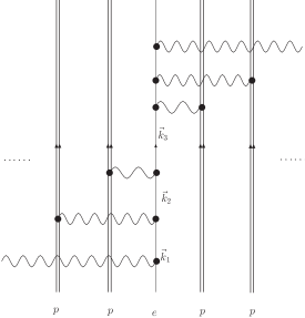
Figure 1: Feynman diagram in which an electron interacts with surrounding protons.

The average number of Rutherford scatterings in the distance $l$, $N$, is given by

$$N={l\over l_{\text{Th}}}.$$ (29)

Thus, the electron’s spread obtains contributions from the proton’s momentum spread $N$ times in the distance $l$. A photon obtains contributions from the electron’s momentum spread. As shown in Appendix B, the momentum spreads of the electron and photon, after the $N$ step of interactions, are given by

$$(\Delta p_{\text{total}})^{2}=\sum_{i}^{N}(\Delta p_{i})^{2},$$ (30)

and its magnitude becomes large for large $N$. Particularly if $(\Delta p_{i})^{2}=(\Delta p)^{2}$ is finite, $(\Delta p_{\text{total}})^{2}$ is given by

$$(\Delta p_{\text{total}})^{2}=N(\Delta p)^{2}$$ (31)

and reaches the absolute value of the momentum, $|p|$, at a sufficiently large $N$. This is realized at a macroscopic distance $l$. Thus, the total spread becomes

$$\Delta p_{\text{total}}\rightarrow\infty,$$ (32)

and the wave has a large momentum spread and the momentum conservation becomes effectively negligible.

Next, we focus the final Thomson scattering of one photon and one electron shown in Fig. 2. The incoming states of the final scattering are almost real photon and electron and have large momentum spreads. These photon and electron are described by superpositions of momentum states of large momentum uncertainties with a suitable energy weight.

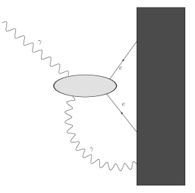
Figure 2: Final Thomson scattering in which one photon and one electron interact and the photon in the final state is detected. The black box shows many-particle states.

2.2.2 Statistical model

The weight of the superposition of the initial states at the final scattering is determined using its previous scatterings and identical particle effects. From the facts that the waves have large momentum spreads after the macroscopic distance and that the amplitude of the Thomson scattering in low energy of the range 3000 - 4000 K is constant and spherically symmetric, waves of the photon and electron in the initial state of the final scattering are regarded as spherical waves that are superpositions of plane waves of all orientations.

In the many-particle state, identical particles satisfy either Fermi-Dirac statistics or Bose-Einstein statistics, and the total energy conservation law

$$\sum_{i}^{N}n_{i}E_{i}=E,$$ (33)

is satisfied. An average occupation number of the state ${\vec{p}}$, i.e., one particle distribution, is given by Bose-Einstein distribution

$$n_{\text{P}}({\vec{p}})=N_{\text{BE}}({\vec{p}})={1\over e^{\frac{p^{0}}{k_{\text{B}}T}}-1}$$ (34)

for photon and by Fermi-Dirac distribution

$$n_{e}({\vec{p}})=N_{\text{FD}}({\vec{p}})={1\over e^{{p^{0}-\mu}\over k_{\text{B}}T}+1}$$ (35)

for electron, where $\mu$ is the chemical potential, $k_{\text{B}}$ is Boltzmann constant, and $T$ is the temperature that is determined from the average energy. A many-body wave function that satisfies these conditions mentioned above is the coherent state of the Boson field and the state of the Fermi field constructed in the same manner. An explicit form is given in Appendix C.

Thus, we assume that the amplitude for one photon and one electron is given by

$$T(1)=N_{\text{BE}}(p_{2})^{1/2}N_{\text{FD}}(k_{2})^{1/2}\tilde{T}(1),$$ (36)

where $\tilde{T}(1)$ does not depend on ${\vec{p}_{2}}$ and ${\vec{k}_{2}}$. The whole amplitude is written as

$$T({\vec{k}}_{1},{\vec{p}}_{1}) = \int d{\vec{k}}_{2}d{\vec{p}}_{2}T({\vec{p}}_{1},{\vec{k}}_{1};{\vec{p}}_{2},{\vec{k}}_{2})N_{\text{F}}(p_{2})^{1/2}N_{\text{B}}(k_{2})^{1/2}\delta({\vec{p}}_{2}+{\vec{k}}_{2}-{\vec{p}}_{1}-{\vec{k}}_{1})$$ (37)

$$\times\tilde{T}(1),$$

where $T({\vec{p}}_{1},{\vec{k}}_{1};{\vec{p}}_{2},{\vec{k}}_{2})$ is the amplitude of Thomson scattering and is constant in low energy.

The momentum correlation function $C({\vec{p}}_{1},{\vec{p}}_{2})$ is a product of the amplitude of the photon momentum ${\vec{p}}_{1}$ and its complex conjugate of the photon momentum ${\vec{p}}_{2}$ and is given by

$$C({\vec{k}}_{1},{\vec{k}^{\prime}}_{1})=\int d{\vec{k}}_{2}d{\vec{p}}_{2}T({\vec{p}}_{1},{\vec{k}}_{1};{\vec{p}}_{2},{\vec{k}}_{2})N_{\text{F}}(p_{2})^{1/2}N_{\text{B}}(k_{2})^{1/2}\delta({\vec{p}}_{2}+{\vec{k}}_{2}-{\vec{p}}_{1}-{\vec{k}}_{1})$$

$$\int d{\vec{k}}^{\prime}_{2}d{\vec{p}}^{\prime}_{2}T({\vec{p}}^{\prime}_{1},{\vec{k}}_{1};{\vec{p}}^{\prime}_{2},{\vec{k}}^{\prime}_{2})N_{\text{F}}(p^{\prime}_{2})^{1/2}N_{\text{B}}(k^{\prime}_{2})^{1/2}\delta({\vec{p}}^{\prime}_{2}+{\vec{k}}^{\prime}_{2}-{\vec{p}}_{1}-{\vec{k}}^{\prime}_{1})|\tilde{T}|^{2}.$$ (38)

This correlation $C({\vec{k}}_{1},{\vec{k}^{\prime}}_{1})$ shows the wave packet nature of photons.

We compute the above function $C({\vec{k}}_{1},{\vec{k}^{\prime}}_{1})$ numerically. The result is given in Fig. 3.

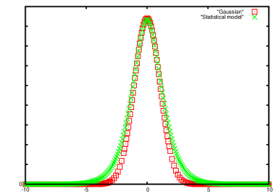
Figure 3: The photon correlation function of a statistical model shown by crosses is compared with a Gaussian function shown by boxes. The width of the Gaussian function is about 3.5$k_{B}T$ and $T=3500$K.

As seen from Fig. 3, the correlation shows that of a Gaussian wave packet of the width of $3.5k_{\text{B}}T$. The photon is regarded as a wave packet whose energy distribution is a Planck distribution but the momentum width is $3.5k_{\text{B}}T$. This wave packet size should be understood as a maximal possible value. The effect of the wave packet is show in Ref. Ishikawa-Tobita.

2.3 Measurements of particle’s trajectory

When a particle is measured using an apparatus, its position and momentum are measured within certain uncertainties. Many physical processes are involved in measurements, but regardless of these processes when the position and momentum are determined within uncertainties, the final state after the measurement is expressed as the state with these uncertainties. Thus, a wave packet of suitable values of momentum width and coordinate width is used for this state. The probability for the particle to be observed within these widths of wave packet is unity, and it follows a classical motion before the next measurement.

The product of uncertainties of the momentum $\Delta{\vec{p}}$ and position $\Delta{\vec{x}}$ may be much larger than that of the minimum wave packet,

$$|\Delta{\vec{x}}||\Delta{\vec{p}}|\gg{\hbar\over 2},$$ (39)

so nonminimum wave packets $\left(\text{Eq}.~{}(\ref{non-minumum-wave packet})\right)$ are suitable for these states.

By successive measurements, a particle’s trajectory that follows classical motion is observed [15]. This happens because the wave packet has a finite spatial size, and the probability for this particle to be observed in the inside of this region is unity. Actually, as discussed in a previous paper,[5] the wave packet spreads with time. The spreading velocity depends on the mass and energy. For the particle trajectory to be observed, a next successive reaction with an apparatus should occur before the wave becomes large. Unless an observation is made, the wave spreads ultimately and a straight trajectory is not tested.

Because light microscopic particles spread fast, they become momentum eigenstates easily. Hence, translational invariance is preserved for these particles. On the other hand, for macroscopic objects or extremely heavy particles, the spreading velocities are negligible and they are localized at certain positions of the initial states. Translational invariance is violated for these objects.

3 Potential scatterings

In this section, we study the scatterings of the wave packets using simple rectangular potentials. We see that the sizes of extensions in the positions and momenta have strong correlations with the velocities of the wave packets and the products of both sizes are approximately adiabatic invariants. Minimum wave packets are changed to nonminimum wave packets in certain reactions.

3.1 Potential wall in one dimension

We study the wave packets first in a simple potential, i.e., in a constant potential wall of a height or depth $V_{0}$ described by

$$U(x)=\begin{cases}V_{0},\ x\leq 0,\\ 0,\ \ 0<x.\end{cases}$$ (40)

We obtain a solution of Schrödinger equation,

$$i\hbar{\partial\over\partial t}\psi(x,t)=H\psi(x,t),$$ (41)

$$H={p^{2}\over 2m}+U(x),$$ (42)

of the following form,

$$\psi(x,t) = e^{Et\over i\hbar}\psi(x),$$ (43)

$$\psi(x) = \begin{cases}e^{ikx}+B_{-}e^{-ikx},~{}x<0,\\ C_{+}e^{ik^{\prime}x},~{}0<x,\end{cases}$$ (44)

where at $x<0$, a right-moving plane wave comes in toward the wall and a left-moving wave of magnitude $B_{-}$ is reflected, and at $x>0$, a right-moving wave of magnitude $C_{+}$ is refracted. The parameters $k$ and $k^{\prime}$ are connected with the energy as

$$E={p^{2}\over 2m}+V_{0}={p^{\prime 2}\over 2m},$$ (45)

$$p=\hbar k,~{}p^{\prime}=\hbar k^{\prime}.$$ (46)

The coefficients are found from the continuities of the wave function at $x=0$ as [16]

$$B_{-}={k-k^{\prime}\over k+k^{\prime}},$$ (47)

$$C_{+}={2k\over k+k^{\prime}}.$$ (48)

The time-dependent wave packet is constructed using a linear combination of the above waves,

$$\psi_{wp} = \psi_{wp}^{1}+\psi_{wp}^{2}+\psi_{wp}^{3},$$ (49)

$$\psi_{wp}^{1} = \int dk\tilde{N}(k)e^{ik(x-X_{0})}e^{Et\over i\hbar},x<0,$$ (50)

$$\psi_{wp}^{2} =\int dk\tilde{N}(k)\left({k-k^{\prime}\over k+k^{\prime}}\right)e^{-ik(x-X_{0})}e^{Et\over i\hbar},x<0,$$ (51)

$$\psi_{wp}^{3} =\int dk\tilde{N}(k)\left({2k\over k+k^{\prime}}\right)e^{ik^{\prime}(x-X_{0})}e^{Et\over i\hbar},0<x,$$ (52)

where

$$\tilde{N}(k) = N_{1}e^{-{(k-k_{0})^{2}\over 2\sigma}},$$ (53)

$$N_{1} = {1\over\sqrt{2\sigma\pi}}.$$ (54)

The wave packet $\psi_{wp}^{1}$ is a minimum wave packet, but the wave packets $\psi_{wp}^{2}$ and $\psi_{wp}^{3}$ are not minimum wave packets owing to the momentum-dependent factors in the amplitudes, ${{k-k^{\prime}\over k+k^{\prime}},{2k\over k+k^{\prime}}}$.

$$\delta x^{1}\times\delta p^{1}={\hbar\over 2},$$ (55)

$$\delta x^{2}\times\delta p^{2}=(1.2\sim 1.4)\times{\hbar\over 2},$$ (56)

$$\delta x^{3}\times\delta p^{3}=(1.0\sim 3.0)\times{\hbar\over 2}.$$ (57)

The initial wave packet is chosen to be minimum and satisfies the minimum uncertainty relation, and the reflected wave and accelerated wave have uncertainty relations of about twice the minimum. In particular, the value of $\delta x\delta p$ for the accelerated wave depends on the potential depth, as given in Fig. 4. The product of uncertainties becomes $\frac{1}{2}\hbar$ at $V_{0}\rightarrow\infty$ and $\frac{3}{2}\hbar$ at $V_{0}\rightarrow 0$. This is because the wave function behaves in these regions as

$$\psi_{wp}^{3}\propto\begin{cases}k\times e^{-\frac{k^{2}}{2\sigma}},\ \ V_{0}\ll E_{0},\\ \text{const}\times e^{-\frac{k^{2}}{2\sigma}},\ \ V_{0}\gg E_{0},\end{cases}$$ (58)

just like a wave function for a ground state and a first excited state of a harmonic oscillator in Eq. (10). The product of uncertainties of the accelerated wave is changed smoothly as seen in Fig. 4.

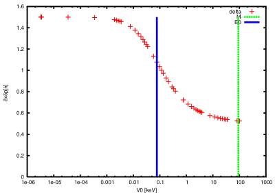
Figure 4: The numerical value of $\delta x\times\delta p$ as a function of the potential depth, $V_{0}$, for accelerated wave packet is given. The horizontal axis shows the potential depth and the vertical axis shows $\delta x\times\delta p$. “delta” is for a numerical result, $E_{0}$ is average energy and M is mass.

3.2 Potential barrier

We study wave packets next in a simple potential, i.e., in a constant potential barrier of finite width $a$ and height or depth $V_{0}$ described as

$$U(x)=\begin{cases}0,~{}x\leq 0,\\ -V_{0},~{}0\leq x\leq a,\\ 0,~{}a\leq x.\end{cases}$$ (59)

We obtain a wave function of the following form:

$$\psi(x)=\begin{cases}e^{i{1\over\hbar}\sqrt{2mE}x}+B_{-}e^{-i{1\over\hbar}\sqrt{2mE}x},~{}x<0,\\ =A_{+}e^{{i\over\hbar}\sqrt{2m(E+V_{0})}x}+A_{-}e^{-{i\over\hbar}\sqrt{2m(E+V_{0})}x},~{}0<x<a,\\ =C_{+}e^{i{1\over\hbar}\sqrt{2mE}x},~{}a<x,\end{cases}$$ (60)

where at $x<0$, a right-moving plane wave comes in and a reflected left-moving wave of magnitude $B_{-}$ is reflected, and at $x>a$, a right-moving wave of magnitude $C_{+}$ is refracted. Coefficients $A_{i}$ show the magnitude in the inside of potential, $0<x<a$. These coefficients are found as [16]

$$A_{+}=2{1+\sqrt{1+V_{0}/E}\over(1+\sqrt{1+V_{0}/E})^{2}-(1-\sqrt{1+V_{0}/E})^{2}e^{2{i\over\hbar}\sqrt{2m(E+V_{0})}a}},$$ (61)

$$A_{-}=2{(-1+\sqrt{1+V_{0}/E})e^{2{i\over\hbar}\sqrt{2m(E+V_{0})}a}\over(1+\sqrt{1+V_{0}/E})^{2}-(1-\sqrt{1+V_{0}/E})^{2}e^{2{i\over\hbar}\sqrt{2m(E+V_{0})}a}},$$ (62)

and coefficients $B_{-},C_{+}$ are found as

$$B_{-} = 1-2{{\sqrt{1+V_{0}/E}+1+V_{0}/E+(\sqrt{1+V_{0}/E}-1-V_{0}/E)}e^{2{i\over\hbar}\sqrt{2m(E+V_{0})}a}\over(1+\sqrt{1+V_{0}/E})^{2}-(1-\sqrt{1+V_{0}/E})^{2}e^{2{i\over\hbar}\sqrt{2m(E+V_{0})}a}},$$

$$C_{+} = 2{(1+\sqrt{1+V_{0}/E})+(-1+\sqrt{1+V_{0}/E})e^{{i\over\hbar}\sqrt{2m(E+V_{0})}a}\over(1+\sqrt{1+V_{0}/E})^{2}-(1-\sqrt{1+V_{0}/E})^{2}e^{2{i\over\hbar}\sqrt{2m(E+V_{0})}a}}$$ (64)

$$\times e^{{i\over\hbar}(\sqrt{2m(E+V_{0})}a-\sqrt{2mE}a)}.$$

Wave packets at $x>0$ and $x<0$ are computed as

$$\psi_{wp}^{1} = \int dk~{}N(k)e^{i(kx-\frac{Et}{\hbar})},~{}x\ll 0,$$ (65)

$$\psi_{wp}^{2} = \int dk~{}N(k)B_{-}(k)e^{-i(kx+\frac{Et}{\hbar})},~{}x\ll 0,$$ (66)

$$\psi_{wp}^{3} = \int dk~{}N(k)C_{+}(k)e^{i(kx-\frac{Et}{\hbar})},~{}x\gg 0,$$ (67)

where $N(k)$ is given in Eq. $(\ref{normalization})$.

Wave packets $\psi_{wp}^{i}(i=1-3)$ are computed numerically. In the negative $x$ region, the minimum wave packet comes in, and refracted and reflected wave packets are generated. The variances of $\psi_{wp}^{1}$, $\psi_{wp}^{2}$, and $\psi_{wp}^{3}$ are computed numerically and are given by

$$\delta x^{1}\times\delta p^{1}=\frac{\hbar}{2},$$ (68)

$$\delta x^{2}\times\delta p^{2}=(1.0\sim 1.6)\times\frac{\hbar}{2},$$ (69)

$$\delta x^{3}\times\delta p^{3}\simeq\frac{\hbar}{2}.$$ (70)

The numerical result for $\psi_{wp}^{3}$ is shown in Fig. 5, where we set $\delta x^{1}=8.0\times 10^{-10}[\text{m}]$, and the width of the potential is taken from 0 to $1.5\times\delta x^{1}$ and the potential depth is of the order of the average energy of the wave packet. In this region,  $\delta x^{3}\times\delta p^{3}$ is approximately adiabatic invariant and the minimum wave packet remains nearly minimum after potential scattering. On the other hand, $\delta x^{2}\times\delta p^{2}$ becomes large. The large change of $\delta x^{2}\times\delta p^{2}$ from $\delta x^{1}\times\delta p^{1}$ is generated, because there are two boundaries of the potential barrier/well.

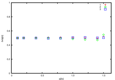
Figure 5: $\delta x^{3}\times\delta p^{3}$ is given as a function of the potential width. The horizontal axis shows the potential width and the vertical axis shows $\delta x\times\delta p$. 1 is for $V_{0}=E_{0}$, 2 is for $V_{0}=\frac{3}{2}E_{0}$, and 3 is for $V_{0}=\frac{1}{2}E_{0}$, where $E_{0}$ is the average energy of the wave packet.

3.3 Potential scatterings in three dimensions

The Schrödinger equation with a one-dimensional potential $U(z)$

$$\left[-{{\hbar}^{2}\over 2m}{\vec{\nabla}}^{2}+U(z)\right]\psi({\vec{x}})=E\psi({\vec{x}})$$ (71)

has solutions of the form,

$$\psi({\vec{x}})=e^{i{\vec{p}}_{T}\cdot{\vec{x}}_{T}}u(z).$$ (72)

The first part on the right-hand side is the plane wave in the transverse direction ${\vec{p}}_{T}=(p_{x},p_{y}),{\vec{x}}_{T}=(x,y)$ and the second part is the function of $z$.

The wave packet is formed from the above wave function as

$$\psi_{wp}=\int d{\vec{k}}_{T}N({\vec{k}-k_{0}}_{T})e^{i{\vec{p}}_{T}\cdot{\vec{x}}_{T}}\int dk_{z}N(k_{z}-k_{z}^{0})u(z),$$ (73)

where the wave packet in the transverse direction is the wave packet of the free wave, and the wave packet in the $z$ direction is the wave packet of the scattering wave in the one-dimensional potentials studied in the previous section.

The wave packet is modified by potentials in the direction of the one-dimensional potential and is not modified in the transverse directions. The time-dependent wave packet is given by

$$\psi({\vec{x}},t)=\int d{\vec{k}}_{T}N({\vec{k}-k_{0}}_{T})dk_{z}N(k-k_{z}^{0})e^{i{\vec{p}}_{T}\cdot{\vec{x}}_{T}}u(z)e^{-iE({\vec{p}}_{T},p_{z})t}.$$ (74)

Obviously, at small $t$, the momentum width in the transverse direction is not modified, but the momentum width in the longitudinal direction is modified by the potential. The change in the width in the longitudinal direction is similar to that of one dimension.

4 Transformations of wave packets

In this section, we study the transformations of wave packets and find changes in wave packets under various transformations based on semiclassical treatments. We assume that the transition of wave packets is smooth and continuous in momentum, and naive treatment of the wave packet’s parameters is possible. In these calculations, singular behaviors of the scattering amplitudes such as resonances are excluded.

4.1 Lorentz transformation

By a Lorentz transformation, a momentum $p_{\nu}$ is transformed to $p^{\prime}_{\nu}$ using a matrix

$${p_{\mu}}^{\prime}=\Lambda^{\mu\nu}p_{\nu}.$$ (75)

The momentum in the direction of the boost is transformed together with the energy, but the momentum in the transverse direction is unchanged. The variances of the momentum components are transformed in the same manner.

The amplitude for the plane wave is known to be covariant under the Lorentz transformation, but the present amplitude for the wave packets has a noninvariant part, because the wave packet size is not fully covariant.

4.2 Addition of potential energy

In a potential scattering, one particle obtains energy from a potential $V_{0}$

$$E_{1}=E_{2}+V_{0},$$ (76)

so wave packet parameters are transformed when a wave packet passes a potential.

4.2.1 Nonrelativistic case

For a nonrelativistic particle, momenta are related by

$$({\vec{p}}_{1})^{2}+2mV_{0}=({\vec{p}}_{2})^{2}.$$ (77)

By decomposing the momentum vector into the longitudinal component and the transverse component and their small deviations,

$$(\delta p_{1}^{l}+p_{1}^{(0)})^{2}+({\delta{\vec{p}}_{1}^{T}})^{2}+2mV_{0}=(\delta p_{1}^{l}+p_{2}^{(0)})^{2}+({\delta{\vec{p}}_{1}^{T}})^{2},$$ (78)

we have equalities for the central values and variances of the momenta

$$(p_{1}^{(0)})^{2}+2mV_{0}=(p_{2}^{(0)})^{2},$$ (79)

$$2p_{1}^{(0)}\delta p_{1}^{l}=2p_{2}^{(0)}\delta p_{2}^{l},$$ (80)

$$({\delta p_{1}^{T}})^{2}=({\delta p_{2}^{T}})^{2}.$$ (81)

Thus, the variances of momenta are connected by

$${\delta p_{1}^{l}\over\delta p_{2}^{l}}={p_{2}^{0}\over p_{1}^{0}}.$$ (82)

By using the time duration $\tau$, the spatial sizes in the longitudinal direction are proportional to the central value of the velocity,

$$\delta x_{1}^{l}=v_{1}^{l}\tau,v_{1}^{l}={p_{1}^{0}\over m},$$ (83)

$$\delta x_{2}^{l}=v_{2}^{l}\tau,v_{1}^{l}={p_{1}^{0}\over m},$$ (84)

hence, the ratio satisfies

$${\delta x_{1}^{l}\over\delta x_{2}^{l}}={p_{1}^{0}\over p_{2}^{0}}.$$ (85)

From Eqs. (82) and (85), the product of momentum extensions and position extensions becomes adiabatic invariant,

$${\delta x_{1}^{l}\delta p_{1}^{l}\over\delta x_{2}^{l}\delta p_{2}^{l}}=\text{constant}.$$ (86)

The momentum extensions and spatial sizes in the transverse direction are unchanged

$$\delta x_{1}^{T}={\hbar\over\delta p_{1}^{T}}={\hbar\over\delta p_{2}^{T}}{\delta p_{2}^{T}\over\delta p_{1}^{T}}=\delta x_{2}^{T}$$ (87)

and are proportional to their energies.

4.2.2 Relativistic case

For the relativistic particle, the relation is modified to

$$\sqrt{(\delta p_{1}^{l}+p_{1}^{(0)})^{2}+({\delta{\vec{p}}_{1}^{T}})^{2}+m^{2}}=\sqrt{(\delta p_{2}^{l}+p_{2}^{(0)})^{2}+({\delta{\vec{p}}_{2}^{T}})^{2}+m^{2}}+V_{0}.$$ (88)

Thus, we have

$$\sqrt{(p_{1}^{(0)})^{2}+m^{2}}=\sqrt{(p_{2}^{(0)})^{2}+m^{2}}+V_{0},$$ (89)

$$2{p_{1}^{(0)}\over E_{1}}\delta p_{1}^{l}=2{p_{2}^{(0)}\over E_{2}}\delta p_{2}^{l},$$ (90)

$$({\vec{\delta}p_{1}}^{T})^{2}=({\vec{\delta}p_{2}}^{T})^{2},$$ (91)

hence, the spatial sizes of extensions in the longitudinal direction are given by

$$\delta x_{1}^{l}={\hbar\over\delta p_{1}^{l}}={\hbar\over\delta p_{2}^{l}}{\delta p_{2}^{l}\over\delta p_{1}^{l}}={{p_{1}^{l}\over E_{1}}\over{p_{2}^{l}\over E_{2}}}\delta x_{2}^{l}.$$ (92)

The momentum extensions and spatial sizes in the transverse direction are unchanged

$$\delta x_{1}^{T}={\hbar\over\delta p_{1}^{T}}={\hbar\over\delta p_{2}^{T}}{\delta p_{2}^{T}\over\delta p_{1}^{T}}=\delta x_{2}^{T}.$$ (93)

In the low-energy region, the energy $E_{1}$ and $E_{2}$ are $mc^{2}$ and the relation of the spatial extensions coincides with that of the nonrelativistic case, Eq. $(\ref{ratio-widths-nonrelativistic-T})$. If both momenta are relativistic, the velocities are almost $c$,

$${p_{1}\over E_{1}}={p_{2}\over E_{2}}=c$$ (94)

and both sizes are almost the same,

$$\delta x_{1}=\delta x_{2}.$$ (95)

The massless particle has a light velocity and does not spread in the direction of motion, and the massive particle has the same property, that is, the coherence length is not transformed in the relativistic regime. On the other hand, the massive particle expands when its energy is enlarged by the potential energy from the nonrelativistic region to the relativistic region and has a size at light velocity,

$$\delta x_{c}={c\over v}\delta x_{v}$$ (96)

if it has $\delta x_{v}$ at velocity $v$.

4.3 Scale transformation

In scale transformation, a momentum is multiplied by a constant factor $\lambda$,

$${p_{\mu}}_{2}=\lambda{p_{\mu}}_{1},$$ (97)

which is consistent with the energy and momentum relation of the massless particle. Thus, this transformation is applied only to the massless particle.

The variance is transformed then by

$$\delta{p_{\mu}}_{2}=\lambda\delta{p_{\mu}}_{1},$$ (98)

hence, the spatial sizes of extensions are given by

$$\delta{x_{\mu}}_{2}={1\over\lambda}\delta{x_{\mu}}_{1}.$$ (99)

For $\lambda<<1$, we have

$$\delta x_{2}>>\delta x_{1}.$$ (100)

5 Refraction and reflection

We study situations where a half space is occupied by one medium and another half is occupied by another medium. A wave packet in one half is reflected at the other half and refracted at the boundary. Wave packets of these situations are studied here.

In the situation where one half is the vacuum and another half is filled with medium, the wave in the medium has a mean free path. Thus, the wave that is produced in the medium first and emitted into the vacuum later is described using a wave of finite coherence length. Although the wave in the vacuum is described using the free Hamiltonian, this wave is the wave packet of having a finite mean free time and a finite energy width. Thus, the sizes of wave packets in vacuum are determined using the mean free path in the medium if the wave is produced in the medium and emitted into the vacuum.

5.1 Electrons from metal to vacuum

Electrons in the metal follow energy dispersions that are characteristic of the band structure and have a lower energy than that in the vacuum because of the value of the work function. The energy dispersion is approximately expressed by a quadratic form of an effective mass $m_{\text{eff}}$ that is different from the mass in the vacuum $m_{0}$. For a spherically symmetric band, we have the relation of energies between the momentum in metal ${\vec{p}}_{1}$ and the momentum in vacuum ${\vec{p}}_{2}$,

$$E_{0}+{{\vec{p}_{1}}^{2}\over 2m_{\text{eff}}}={{\vec{p}_{2}}^{2}\over 2m_{0}},$$ (101)

where $E_{0}$ is the work function in the metal.

By decomposing the momenta into the components and the central values $p_{i}^{0}$ and deviations in the longitudinal direction, $\delta p_{l}$, and those in the transverse directions, ${\vec{\delta}p}_{i}$, we have

$$E_{0}+{{p_{1}^{0}}^{2}\over 2m_{\text{eff}}}={{p_{2}^{0}}^{2}\over 2m_{0}},$$ (102)

$${2{p_{1}^{0}}\delta p_{1}^{l}\over 2m_{\text{eff}}}={{p_{2}^{0}}\delta p_{2}^{l}\over 2m_{0}},$$ (103)

$${{\delta{\vec{p}}_{1}}^{2}\over 2m_{\text{eff}}}={{\delta{\vec{p}}_{2}}^{2}\over 2m_{0}}.$$ (104)

Electrons propagate in the form of wave packets of the above parameters.

5.2 Lights from medium to vacuum

5.2.1 Without absorption

In an insulator medium, the dielectric constant is different from that in a vacuum and is real if there is no absorption. In this situation, a momentum in the medium ${\vec{p}}_{1}$ and a momentum in the vacuum ${\vec{p}}_{2}$ are connected by

$$c_{m}{p}_{1}=c{p}_{2},$$ (105)

$$c_{m}=c\sqrt{\mu_{0}\epsilon_{0}\over\mu\epsilon},$$ (106)

where $\mu$ and $\mu_{0}$ are the permeabilities of the medium and vacuum and $\epsilon$ and $\epsilon_{0}$ are the dielectric constants of the medium and vacuum, respectively. $c_{m}$ is the light velocity in the medium and $c$ is the light velocity in the vacuum.

5.2.2 Finite absorption

In a system of absorption, the photon energy has an imaginary part

$$\Gamma=\mu{1\over\rho},$$ (107)

where $\rho$ is resistivity. The relation of the momenta at the boundary is given by

$$c_{m}{p}_{1}=c{p}_{2},$$ (108)

$$c_{m}=c\sqrt{\mu_{0}\epsilon_{0}\over\mu\epsilon},$$ (109)

but owing to the imaginary part of the energy, the wave lives for a finite time $\tau$

$$\tau={\epsilon\rho}$$ (110)

in the medium. Thus, the light that is emitted from the medium into the vacuum has an uncertainty of energy $\Delta E$,

$$\Delta E={\hbar\over\tau}.$$ (111)

Lights propagate in the form of wave packets of the above parameters.

6 Many-body processes

The coherence length of a particle in final states of many-body processes is determined on the basis of the uncertainties of the energy and momentum of the initial states. The momentum correlation (Eq. (13)) of a one-particle state is used for obtaining the coherence length.

6.1 Two-body decay

In a two-body decay, $A\rightarrow B+C$, the energy and magnitude of momentum of B and C are fixed in the rest system of A. The correlation function (Eq. $(\ref{correlation-wave packet})$) is defined as

$$C({\vec{p}}_{1},{\vec{p}}_{2})=\sum_{{\vec{p}}_{C}}\langle{\vec{p}}_{1},{\vec{p}}_{C}|T|A\rangle(\langle{\vec{p}}_{2},{\vec{p}}_{C}|T|A\rangle)^{*},$$ (112)

where the above amplitude is proportional to the amplitude $\tilde{T}$ and the delta function of energy momentum conservation,

$$\langle{\vec{p}}_{1},{\vec{p}}_{C}|T|A\rangle=\delta^{4}({p}_{A}-{p}_{1}-{p}_{C})\tilde{T}$$ (113)

when the state $A$ is the eigenstate of the energy and momentum. Thus, if the state $A$ is the eigenstate of the energy and momentum, the above correlation function becomes proportional to

$$C({\vec{p}}_{1},{\vec{p}}_{2})=\tilde{T}{\tilde{T}}^{*}\delta^{4}({p}_{1}-{p}_{2}).$$ (114)

On the other hand, when the state $A$ is a wave packet of the function $F({\vec{p}}_{A})$, the correlation function is given by

$$C({\vec{p}}_{1},{\vec{p}}_{2}) = \sum_{{\vec{p}}_{C}}\int d{\vec{p}}_{A}d{\vec{p}}_{A^{\prime}}\langle{\vec{p}}_{1},{\vec{p}}_{C}|T|{\vec{p}}_{A}\rangle(\langle{\vec{p}}_{2},{\vec{p}}_{C}|T|{\vec{p}}_{A}^{\prime}\rangle)^{*}F({\vec{p}}_{A})F^{*}({\vec{p}}_{A^{\prime}})$$ (115)

$$= \int d{\vec{p}}_{A}d{\vec{p}}_{A^{\prime}}\delta({\vec{p}}_{1}-{\vec{p}}_{2}-{\vec{p}}_{A}+{\vec{p}}_{A^{\prime}})F({\vec{p}}_{A})F^{*}({\vec{p}}_{A^{\prime}})\tilde{T}{\tilde{T}}^{*}$$

$$\times\delta({p}_{A}^{0}-{p}_{1}^{0}-{p}_{C}^{0})\delta({p}_{A}^{0}-{p}_{1}^{0}-{p}_{C}^{0})$$

$$= \int d{\vec{p}}_{A}F({\vec{p}}_{A})F^{*}({\vec{p}}_{A}-{\vec{p}}_{2}+{\vec{p}}_{1})\tilde{T}{\tilde{T}}^{*}$$

$$\times\delta({p}_{A}^{0}-{p}_{1}^{0}-{p}_{C}^{0})\delta({p}_{A}^{0}-{p}_{1}^{0}-{p}_{C}^{0}).$$

Thus, the momentum correlation $C({\vec{p}}_{1},{\vec{p}}_{2})$ is determined using the momentum distribution function $F({\vec{p}}_{A})$ of the initial state.

6.2 Three-body decay

In a three-body decay, $A\rightarrow B+C+D$, the energy and magnitude of momentum of B, C and D vary even in the rest system of A. If particle B is measured and the other states are not measured but summed, the result of the correlation function for $B$ is the same as that of two-body decay. The correlation function is given by

$$C({\vec{p}}_{1},{\vec{p}}_{2})=\sum_{{\vec{p}}_{C},{\vec{p}}_{D}}\langle{\vec{p}}_{1},{\vec{p}}_{C},{\vec{p}}_{D}|T|{\vec{p}}_{A}\rangle(\langle{\vec{p}}_{2},{\vec{p}}_{C},{\vec{p}}_{D}|T|{\vec{p}}_{A}\rangle)^{*},$$ (116)

and is proportional to the delta function if the state $A$ is the eigenstate of the energy and momentum,

$$C({\vec{p}}_{1},{\vec{p}}_{2})=\delta^{4}({p}_{1}-{p}_{2})\tilde{T}{\tilde{T}}^{*}.$$ (117)

On the other hand, when the state $A$ is a wave packet of the function $F({\vec{p}}_{A})$, the correlation function is given by

$$C({\vec{p}}_{1},{\vec{p}}_{2}) = \sum_{{\vec{p}}_{C},{\vec{p}}_{D}}\int d{\vec{p}}_{A}d{\vec{p}}_{A^{\prime}}\langle{\vec{p}}_{1},{\vec{p}}_{C},{\vec{p}}_{D}|T|{\vec{p}}_{A}\rangle(\langle{\vec{p}}_{2},{\vec{p}}_{C},{\vec{p}}_{D}|T|{\vec{p}}_{A^{\prime}}\rangle)^{*}F({\vec{p}}_{A})F^{*}({\vec{p}}_{A^{\prime}})$$ (118)

$$= \int d{\vec{p}}_{A}d{\vec{p}}_{A^{\prime}}\delta({\vec{p}}_{1}-{\vec{p}}_{2}-{\vec{p}}_{A}+{\vec{p}}_{A^{\prime}})F({\vec{p}}_{A})F^{*}({\vec{p}}_{A^{\prime}})\tilde{T}{\tilde{T}}^{*}$$

$$= \int d{\vec{p}}_{A}F({\vec{p}}_{A})F^{*}({\vec{p}}_{A}+{\vec{p}}_{2}-{\vec{p}}_{1})\tilde{T}{\tilde{T}}^{*}.$$

Thus, the momentum correlation $C({\vec{p}}_{1},{\vec{p}}_{2})$ is determined by the momentum distribution function $F({\vec{p}}_{A})$ of the initial state $A$.

6.3 Two-body collision

The coherence lengths of collision products are treated in the same manner as the decay products of the previous section and are determined on the basis of the uncertainties of the energy and momentum of the initial states. We study the momentum correlations (Eq. $(\ref{correlation-wave packet})$) of one particle also in the collision products. In a two-body collision, $A+B\rightarrow C+D$, we study the correlation function (Eq. $(\ref{correlation-wave packet})$) defined as

$$C({\vec{p}}_{1},{\vec{p}}_{2})=\sum_{{\vec{p}}_{C}}\langle{\vec{p}}_{1},{\vec{p}}_{C}|T|A,B\rangle(\langle{\vec{p}}_{2},{\vec{p}}_{C}|T|A,B\rangle)^{*},$$ (119)

where the above amplitude is proportional to the amplitude $\tilde{T}$ and the delta function of energy momentum conservation,

$$\langle{\vec{p}}_{1},{\vec{p}}_{C}|T|A,B\rangle=\delta^{4}({p}_{\text{initial}}-{p}_{1}-{p}_{C})\tilde{T},$$ (120)

$$p_{\text{initial}=p_{A}+p_{B}}$$

when states $A$ and $B$ are the eigenstates of the energy and momentum. Thus, if the states $A$ and $B$ are the eigenstates of the energy and momentum, the above correlation function becomes proportional to

$$C({\vec{p}}_{1},{\vec{p}}_{2})=\tilde{T}{\tilde{T}}^{*}\delta^{4}({p}_{1}-{p}_{2}).$$ (121)

On the other hand, when states $A$ and $B$ are wave packets of finite spreads, the wave functions overlap within a finite space-time region,

$$\Delta t_{\text{overlap}}\neq\infty,~{}\Delta{\vec{x}}\neq\infty$$ (122)

and the energy-momentum conservation is slightly violated,

$$\Delta E=E_{i}-E_{f}\neq 0,~{}\Delta{\vec{p}}={\vec{p}}_{i}-{\vec{p}}_{f}\neq 0.$$ (123)

The correlation function is expressed using the wave functions $F({\vec{p}}_{A})$ and $F({\vec{p}}_{B})$ as

$$C({\vec{p}}_{1},{\vec{p}}_{2}) = \sum_{{\vec{p}}_{C}}\int d{\vec{p}}_{A}d{\vec{p}}_{A^{\prime}}\int d{\vec{p}}_{B}d{\vec{p}}_{B^{\prime}}\langle{\vec{p}}_{1},{\vec{p}}_{C}|T|{\vec{p}}_{A},{\vec{p}}_{B}\rangle(\langle{\vec{p}}_{2},{\vec{p}}_{C}|T|{\vec{p}}_{A^{\prime}},{\vec{p}}_{B^{\prime}}\rangle)^{*}$$ (124)

$$\times F({\vec{p}}_{A})F^{*}({\vec{p}}_{A^{\prime}})F({\vec{p}}_{B})F^{*}({\vec{p}}_{B^{\prime}})$$

$$= \int d{\vec{p}}_{A}d{\vec{p}}_{A^{\prime}}d{\vec{p}}_{B}d{\vec{p}}_{B^{\prime}}\delta({\vec{p}}_{1}-{\vec{p}}_{2}-{\vec{p}}_{A}+{\vec{p}}_{A^{\prime}}-{\vec{p}}_{B}+{\vec{p}}_{B^{\prime}})$$

$$\times F({\vec{p}}_{A})F^{*}({\vec{p}}_{A^{\prime}})F({\vec{p}}_{B})F^{*}({\vec{p}}_{B^{\prime}})\tilde{T}{\tilde{T}}^{*}$$

$$= \int d{\vec{p}}_{A}F({\vec{p}}_{A})d{\vec{p}}_{B}F({\vec{p}}_{B})F^{*}({\vec{p}}_{A}-{\vec{p}}_{2}+{\vec{p}}_{1})F^{*}({\vec{p}}_{A}-{\vec{p}}_{2}+{\vec{p}}_{1})\tilde{T}{\tilde{T}}^{*}.$$

Thus, the momentum correlation $C({\vec{p}}_{1},{\vec{p}}_{2})$ is determined using the wave functions of the initial state. This result is also applied to many-body scatterings. The correlation function $C({\vec{p}}_{1},{\vec{p}}_{2})$ was used in §2.2.

7 Summary

In this paper, we showed that one-particle states are described using wave packets of finite coherence lengths, i.e., finite wave packet sizes in various situations. The wave packet size is determined either from a one-particle effect or from a many-particle effect. In the former, a finite mean free path is the origin of the wave packet. The finite mean free path makes one particle have a finite spatial extension and a finite momentum uncertainty. The state of a finite mean free path is a nonstationary state and is varied with time. The state is extended also in energy, and the energy width is determined either from the mean free path or from the mean free time. Two values are consistent with each other. In the latter, a one-particle state is generated as a superposition of plane waves owing to many particle effects and has a correlation with a wave packet. The situation is similar to the fact that a spherical wave is produced by a short range potential. The spherical wave is a superposition of plane waves of different orientations. Usually, a particle is detected using a detector of finite size, and the number of events is determined separately at different angles, so it is difficult to observe directly the coherence of different angles. To test the coherence of different angles directly, a particular detector that responds in a wide orientation may be necessary.

We verified in the latter sections that once particles of finite coherence are produced, the finite coherence propagates and transmits to other particles due to scatterings and many-body effects.

In the next paper, we study various applications of wave packets in interference phenomena in large-scale physics.
 

Appendix A Cross Sections around the Decoupling Time

Around the decoupling time of the early universe, the densities of photon, electron, and proton are given by

$$n_{p} = n_{e}=4\times 10^{17}~{}[\text{m}^{-3}],$$ (125)

$$n_{\gamma} = 10^{9}\times n_{p}.$$ (126)

Scattering cross sections of Thomson scattering and Rutherford scattering are given by

$$\sigma_{\text{Ru}} = 4\pi({e^{2}\over 4\pi\epsilon_{0}mv^{2}})^{2}\log\Lambda=4.4\times 10^{-17}[\text{m}^{2}]\times\log\Lambda,$$

$$\Lambda={\gamma\hbar v4\pi\epsilon_{0}\over e^{2}},~{}mv^{2}=kT,$$

$$\sigma_{\text{Th}} = {8\pi r_{e}^{2}\over 3}=0.6\times 10^{-28}~{}[\text{m}^{2}],$$

$$r_{e}={e^{2}\over 4\pi\epsilon_{0}m_{e}c^{2}},$$

where the cutoff parameter $\log\Lambda=10$ and the temperature $T=3000$ K are used. Hence, the mean free paths are given by

$$l_{\text{Ru}}=5.7\times 10^{-3}~{}[\text{m}],$$ (129)

$$l_{\text{Th}}=5~{}[\text{m}],$$ (130)

and we have

$$N_{\text{T}}={l_{\text{Th}}\over l_{\text{Ru}}}=10^{3}.$$ (131)

Appendix B Total Momentum Uncertainty of N Particles

When a particle is surrounded by N particles and interacts with them coherently, one particle in the final state obtains a total momentum uncertainty from N particles. The total amplitude of this processes is written as

$$f=\int\prod_{i}d{\vec{p}}_{i}F({\vec{p}}_{i})\langle{\vec{q}}_{1},\cdots,{\vec{q}}_{M},|T|{\vec{p}}_{1},\cdots{\vec{p}}_{N}\rangle.$$ (132)

We study the case where all the particle states of the initial state are described using the same wave packet for simplicity. In other cases, the following conclusion is the same.

The product of N Gaussian functions

$$F({\vec{p}}_{1})F({\vec{p}}_{2})\cdots F({\vec{p}}_{N}),$$ (133)

$$F({\vec{p}}_{1})=Ne^{-\sigma({{\vec{p}}_{1}-{\vec{p}}_{1}^{0}})^{2}}$$ (134)

is decomposed into the function of the total momentum ${\vec{p}}_{T}$ and relative momenta ${\vec{p}}_{r}$ as

$$F_{T}({\vec{p}}_{T}-{\vec{p}}_{T}^{0})\prod_{r}F_{r}({\vec{p}}_{r}-{\vec{p}}_{r}^{0}).$$ (135)

In the above function, $F_{T}({\vec{p}}_{T}-{\vec{p}}_{T}^{0})$ is given by

$$F_{T}({\vec{p}}_{T}-{\vec{p}}_{T}^{0})=\tilde{N}e^{-{\sigma\over N}({\vec{p}}_{T}-{\vec{p}}_{T}^{0})^{2}},$$ (136)

$${\vec{p}}_{T}=\sum_{i}{\vec{p}}_{i},~{}{\vec{p}}_{T}^{0}=\sum_{i}{\vec{p}}_{i}^{0},$$ (137)

where $\tilde{N}$ is a normalization constant. Thus, the spread of the total momentum increases with $N$ and becomes ${\sqrt{N}}$ times the spread of one particle. These N particles give the momentum uncertainty ${\sqrt{N}}\Delta p$ to the particle.

Appendix C A Wave Function of Statistical Model

The many-body wave function that has a minimum uncertainty of field operators $\phi({\vec{x}})$ and $\pi({\vec{x}})$ for a Boson

$$\delta\phi_{g}^{2}\delta\pi_{g}^{2}\geq{\hbar^{2}\over 4}\int d{\vec{p}}g^{2}({\vec{p}}),$$ (138)

$$\delta\phi_{g}^{2}=\langle\phi_{g}^{2}\rangle-\langle\phi_{g}\rangle^{2},~{}\delta\pi_{g}^{2}=\langle\pi_{g}^{2}\rangle-\langle\pi_{g}\rangle^{2},~{}$$

$$\phi_{g}=\int d{\vec{p}}\phi({\vec{p}})g({\vec{p}}),$$ (139)

$$\pi_{g}=\int d{\vec{p}}\pi({\vec{p}})g({\vec{p}}),$$ (140)

is a coherent state

$$|\psi\rangle=Ne^{\int d{\vec{p}}g({\vec{p}})a^{\dagger}({\vec{p}})}|0\rangle,$$ (141)

$$N^{2}=e^{-\int d{\vec{p}}|g({\vec{p}})|^{2}}.$$ (142)

This coherent state satisfies

$$\langle\psi|a({\vec{q}})|\psi\rangle=g({\vec{q}}),$$ (143)

$$\langle\psi|a({\vec{q}})^{\dagger}a({\vec{q}})|\psi\rangle=|g({\vec{q}})|^{2},$$ (144)

and the number density agrees with that of our statistical model if

$$|g({\vec{p}})|^{2}=n_{P}({\vec{p}}).$$ (145)

An example of the weight is

$$g({\vec{p}},{\vec{X}})=\sqrt{n_{P}({\vec{p}})}e^{-i{\vec{p}}\cdot{\vec{X}}},$$ (146)

where we choose a suitable vector ${\vec{X}}$. For Fermion $b^{\dagger}({\vec{p}})$, a wave function is chosen in the same manner, and we have

$$|\Psi\rangle=N\prod_{i}e^{\int d{\vec{p}}(f({\vec{p}},{\vec{X}}_{i})a^{\dagger}({\vec{p}})+g({\vec{p}},{\vec{X}}_{i})b^{\dagger}({\vec{p}}))}|0\rangle.$$ (147)

References

• [1] J. A. Yeazell and T. Uzer, The Physics and Chemistry of Wave Packets  (John Wiley & Sons, Inc. New York, 2000).
• [2] M. L. Goldberger and K. M. Watson, Collision Theory (John Wiley & Sons, Inc. New York, 1965).
• [3] R. G. Newton, Scattering Theory of Waves and Particles (Springer-Verlag, New York, 1982).
• [4] T. Sasakawa, Prog. Theor. Phys. Suppl. No. 11, (1959),69. See also, T. Sasakawa, Scattering Theory(in Japanese), (Shokabou, Tokyo, 1991).
• [5] K. Ishikawa and T. Shimomura, Prog. Theor. Phys. 114 (2005), 1201.
• [6] L. Brillouin, Wave Propagation and Group Velocity (Academic Press, New York, 1960).
• [7] C. Giunti, C. W. Kim and U. W. Lee, Phys. Rev. D 44 (1991), 3635.
• [8] S. Nussinov, Phys. Lett. B 63 (1976), 201.
• [9] K. Kiers, N. Nussinov and N. Weisis, Phys. Rev. D 53 (1996), 537.
• [10] L. Stodolsky, Phys. Rev. D 58 (1998), 036006.
• [11] A. Asahara, K. Ishikawa, T. Shimomura, and T. Yabuki, Prog. Theor. Phys. 113 (2005), 385; T. Yabuki and K. Ishikawa, Prog. Theor. Phys. 108 (2002), 347.
• [12] K. Ishikawa and T. Shimomura, “Coherent lunar effect on solar neutrino” Hokkaido University preprint (2005).
• [13] K. Ishikawa and Y. Tobita, “Coherence length of cosmic background radiation enlarges the attenuation length of the ultra-high energy proton” Hokkaido University preprint (2005); “Neutrino mass and mixing” in the 10th Inter. Symp. on “Origin of Matter and Evolution of Galaxies” AIP Conference proceedings 1016 (2008), 329.
• [14] A. Goldberg, H. Schey, and J. L. Schwartz, Am. J. Phys. 35 (1967), 177; L. Schiff, Quantum Mechanics 3rd. ed.(McGraw Hill, New York, 1968) p.106.
• [15] L. Schiff, Quantum Mechanics 3rd. ed.(McGraw Hill, New York, 1968) p.335.
• [16] L. D. Landau and E. M. Lifshitz, Quantum Mechanics 3rd. ed. Translated by J. B. Sykes and J. S. Bell (Butterworth Heinemann, New York, 2003).