Stochastic phase reduction for a general class of noisy limit cycle oscillators

Abstract

We formulate a phase reduction method for a general class of noisy limit cycle oscillators and find that the phase equation is parameterized by the ratio between time scales of the noise and amplitude-relaxation time of the limit cycle. The equation naturally includes previously proposed and mutually exclusive phase equations as special cases. The validity of the theory is numerically confirmed. Using the method, we reveal how noise and its correlation time affect limit cycle oscillations.

Self-sustained oscillations are widely observed in physical, chemical and biological systems kuramoto84 ; winfree01 ; pikovsky01 . The oscillations are often described as limit cycle oscillators. Since limit cycle oscillators show rich and varied properties, they have been extensively studied as a central issue of nonlinear science. Timing of limit cycle oscillation can be described by a single phase variable. The phase reduction method is a powerful analytical tool to approximate high-dimensional limit-cycle dynamics as a closed equation for only the single phase variable kuramoto84 . Based on the phase description, studies have revealed fascinating properties of limit-cycle oscillators like response properties and their collective dynamics ermentrout96 ; acebron05 ; kawamura08 .

While the theory of phase reduction has been developed mainly for deterministic limit cycle oscillators, oscillators in the real world are often exposed to noise. Sources of the noise can be internal fluctuations, background noise and also input signals which have noise-like statistics ermentrout07 . Since noisy limit cycle oscillators also show various nontrivial properties, there have been many recent studies of them teramae ; pikovsky ; nakao ; galan07 ; ermentrout08 ; teramae08 ; lin08 ; yoshimura08 . While the phase-reduction method is among the most useful ways to study the effects of noise on oscillators, two mutually exclusive phase equations have been proposed for a limit cycle oscillator driven by white Gaussian noise. The first one is formally the same as the phase equation obtained from deterministic oscillators and is in a sense a limiting case of colored noise teramae ; pikovsky ; nakao ; galan07 ; ermentrout08 ; teramae08 while the second one has an additional term being proportional to square of noise strength and is the technically correct phase equation for white noise yoshimura08 .

Their relationship and which of them is more appropriate description of noisy physical oscillators have not been addressed in the literature. Rather, it was recently pointed out that both of them fail to describe noisy oscillations in some cases nakao09 . These facts must imply existence of a more appropriate phase equation, which will be a starting point for future research of noisy oscillations. In this letter, we solve these problems by formulating the stochastic phase reduction with careful consideration of relationship between correlation time of the noise and relaxation time of the amplitude of the limit cycle.

Noise in the real world has small but finite correlation time kampen92 . When the correlation time is much smaller than characteristic time scales of the noise-driven system, we can use the white noise description by taking the limit where the correlation time goes to zero. For limit cycle oscillators, this condition might seem to mean that the correlation time is much smaller than the period of oscillation. However, limit cycle oscillators always have other significant time scales, i.e., the rate of attraction of perturbations to the limit cycle. These rates characterize stability of the limit cycle against amplitude perturbation. When the limit cycle is very stable to perturbations, the decay time constant could be as small as the short correlation time of the noise. Since interplay of small time constants can play a crucial role in stochastic dynamical systems, we should carefully consider their relationship when we take the white noise limit for noisy limit cycle oscillators. We employ an Ornstein-Uhlenbeck process which explicitly has a finite time correlation and then take the white noise limit of the process while at the same time keeping track of the time constant for attraction to the limit cycle.

Let us consider a smooth limit cycle oscillator driven by the Ornstein-Uhlenbeck process with the time constant $\tau_{\eta}$,

$$\begin{split}\dot{\bm{X}}&=\bm{F}(\bm{X})+\sigma\bm{G}(\bm{X})\eta(t)\\ \tau_{\eta}\dot{\eta}&=-\eta+\xi(t),\end{split}$$ (1)

where $\bm{X}(t)\in\bm{R}^{N}$ is the state of the oscillator at time $t$, $\bm{F}(\bm{X})$ is its intrinsic dynamics, $\bm{G}(\bm{X})$ is a vector function, $\xi(t)$ is the zero mean white Gaussian noise of unit intensity, $\langle\xi(t)\rangle=0$ and $\langle\xi(t)\xi(s)\rangle=\delta(t-s)$, and then $\eta(t)$ represents the zero mean Ornstein-Uhlenbeck process with correlation time $\tau_{\eta}$, $\langle\eta(t)\eta(s)\rangle=\exp(-|t-s|/\tau_{\eta})/(2\tau_{\eta})$. As we take the limit $\tau_{\eta}\to 0$, $\eta(t)$ approaches the white Gaussian process of unit strength. $\sigma$ represents noise strength. $\bm{F}(\bm{X})$ has a stable limit cycle solution $\bm{X}_{0}(t)$ satisfying $\dot{\bm{X}_{0}}=\bm{F}(\bm{X}_{0})$ with period $T$, $\bm{X}_{0}(t+T)=\bm{X}_{0}(t)$. The phase variable $\phi$ is defined around the limit cycle solution and increases by $T$ for every cycle of $\bm{X}(t)$ along the limit cycle. Thus, intrinsic angular velocity of the phase is equal to one. We introduce the other $N-1$ dimensional coordinates $\bm{\rho}=(\rho_{1},\rho_{2},\dots)$ to describe the $N$ dimensional dynamics of $\bm{X}$ using the coordinate $(\phi,\bm{\rho})$ yoshimura08 . Without loss of generality, we can shift the origin of $\bm{\rho}$ to $\bm{\rho}=0$ on the limit cycle solution. For simplicity of the analysis, we assume that $N=2$. Generalization of results to any values of $N$ is straightforward. We now introduce new variable $y(t)=\eta(t)\sqrt{\tau_{\eta}}$. Unlike $\eta$, $y$ has the steady distribution, $P_{0}(y)=\exp(-y^{2})/\sqrt{\pi}$, which is independent of the correlation time $\tau_{\eta}$. Variable translations from $\bm{X}$ to $(\phi,\rho)$ and from $\eta$ to $y$ gives

$$\begin{split}\dot{\phi}&=1+\sigma h(\phi,\rho)\frac{y}{\sqrt{\tau_{\eta}}}\\ \dot{\rho}&=\frac{1}{\tau_{\rho}(\phi)}f(\phi,\rho)+\sigma g(\phi,\rho)\frac{y}{\sqrt{\tau_{\eta}}}\\ \dot{y}&=-\frac{y}{\tau_{\eta}}+\frac{\xi(t)}{\sqrt{\tau_{\eta}}}.\end{split}$$ (2)

The functions $h$, $f$ and $g$ are defined as $h(\phi,\rho)=\nabla_{\bm{X}}\phi\cdot\bm{G}(\bm{X})|_{\bm{X}=\bm{X}(\phi,\rho)}$, $f(\phi,\rho)/\tau_{\rho}=\nabla_{\bm{X}}\rho\cdot\bm{F}(\bm{X})|_{\bm{X}=\bm{X}(\phi,\rho)}$ and $g(\phi,\rho)=\nabla_{\bm{X}}\rho\cdot\bm{G}(\bm{X})|_{\bm{X}=\bm{X}(\phi,\rho)}$ yoshimura08 . Since the limit cycle at $\rho=0$ is stable, we explicitly introduced amplitude-relaxation time of the limit-cycle as $\tau_{\rho}$, which generally depends on $\phi$ and assumed that $f(\phi,0)=0$ and $\partial f(\phi,0)/\partial\rho=-1$. The value of $\tau_{\rho}$ can be very small if the limit cycle is stiff against amplitude perturbations.

To eliminate the amplitude variable $\rho$ and perform the phase reduction, we assume that the limit cycle is sufficiently stable and take the limit $\tau_{\rho}\to 0$. Simultaneously, we have to take the white noise limit $\tau_{\eta}\to 0$. To consider these two limits at the same time, we take the both limits $\tau_{\rho}\to 0$ and $\tau_{\eta}\to 0$ simultaneously keeping the ratio $k=\tau_{\eta}/\tau_{\rho}$ constant. Introducing a small parameter $\epsilon=\sqrt{\tau_{\eta}}$, we translate the variable $\rho$ to $r=\rho/\epsilon$, which remains $O(1)$ as $\epsilon\to 0$. Expanding $h$, $f$ and $g$ as $h(\phi,\epsilon r)=h_{0}(\phi)+h_{1}(\phi)\epsilon r+h_{2}(\phi)\epsilon^{2}r^{2}+\dots$, $f(\phi,\epsilon r)=-\epsilon r+f_{2}(\phi)\epsilon^{2}r^{2}+f_{3}(\phi)\epsilon^{3}r^{3}+\dots$ and $g(\phi,\epsilon r)=g_{0}(\phi)+g_{1}(\phi)\epsilon r+g_{2}(\phi)\epsilon^{2}r^{2}+\dots$, we obtain the Fokker-Planck equation horsthemke84 ; gardiner86 for the distribution function $Q(\phi,r,y,t)$ from the stochastic differential equation Eq.(2) as

$$\epsilon^{2}\frac{\partial Q}{\partial t}=(L_{0}-\epsilon L_{1}-\epsilon^{2}L_{2})Q+O(\epsilon^{3}),$$ (3)

where linear operators are defined as $L_{0}Q=(yQ)_{y}+Q_{yy}/2+k(rQ)_{r}-\sigma yg_{0}Q_{r}$, $L_{1}Q=\sigma y[g_{1}(rQ)_{r}+(h_{0}Q)_{\phi}]+kf_{2}(r^{2}Q)_{r}$ and $L_{2}Q=\sigma y[g_{2}(r^{2}Q)_{r}+r(h_{1}Q)_{\phi}]+Q_{\phi}+kf_{3}(r^{3}Q)_{r}$. Subscript $x$ means partial derivative with respect to the variable $x$. We assume that $Q$ vanishes rapidly as $y\to\pm\infty$ or $r\to\pm\infty$. Expanding $Q$ in a perturbation series in $\epsilon$, $Q=Q_{0}+\epsilon Q_{1}+\epsilon^{2}Q_{2}+\dots$, and equating coefficients of equal power of $\epsilon$ in Eq. (3), we obtain

$$\epsilon^{0}:L_{0}Q_{0} =0$$ (4)

$$\epsilon^{1}:L_{0}Q_{1} =L_{1}Q_{0}$$ (5)

$$\epsilon^{2}:L_{0}Q_{2} =\frac{\partial}{\partial t}Q_{0}+L_{2}Q_{0}+L_{1}Q_{1}.$$ (6)

The lowest order equation, Eq. (4), has a solution, $Q_{0}=P(\phi,t)W(\phi,r,y)$, where $W(\phi,r,y)=\sqrt{k}(1+k)/(\sigma g_{0}\pi)\exp(-y^{2}-k(y-(1+k)r/(\sigma g_{0}))^{2})$ is the steady Gaussian distribution function of $r$ and $y$ with frozen $\phi$ and $g(\phi,r)=g_{0}(\phi)$. $P(\phi,t)$ is the distribution function of the $\phi$. Our primary goal is to find the evolution equation for $P$, which is nothing but the reduced Fokker-Planck equation for the phase variable $\phi$ horsthemke84 ; gardiner86 .

Since the linear operator $L_{0}$ has the zero eigenvalue, Eq. (5) and (6) have to fulfill a solvability condition known as the Fredholm alternative. That is, $L_{0}U=b$ has a solution if and only if, $b$ is orthogonal to the nullspace of the adjoint of $L_{0}.$ This nullspace is simply the constant function 1. Thus we can solve $L_{0}U=b$ when the integral of $b$ over $(r,y)$ vanishes. To obtain this condition, we integrate both sides of these equations with respect to both $r$ and $y$ from $-\infty$ to $\infty$. We will see that the condition for Eq. (6) is nothing but the desired Fokker-Planck equation for $\phi$. Equation (5) is solvable since integration over $(r,y)$ is zero. To see why, note that integration of the term $(rQ_{0})_{r}$ with respect to $r$ vanishes since $rQ_{0}(r,y)$ vanishes as $|r|\to\infty.$ Integration of $yQ_{0}(y,r)$ first with repect to $r$ yields an odd function of $y$ which is absolutely integrable and thus its integral over $y$ vanishes. We do not need the full expression for $Q_{1}$ at this point, so defer its calculation to the next step. Integration of Eq. (6) gives

$$0=P_{t}+\sigma\left[h_{0}\int_{-\infty}^{\infty}\int_{-\infty}^{\infty}(yQ_{1})drdy+\frac{\sigma g_{0}}{2(1+k)}h_{1}P\right]_{\phi}+P_{\phi},$$ (7)

where we used the rapidly vanishing assumption of $Q$. The coefficient of the 3rd term comes from the relationship $\int_{-\infty}^{\infty}\int_{-\infty}^{\infty}(yrW)drdy=\sigma g_{0}/\left(2\left(1+k\right)\right)$, which is the correlation between $y$ and $r$ for fixed $\phi$. To evaluate $\int_{-\infty}^{\infty}\int_{-\infty}^{\infty}(yQ_{1})drdy$ of the 2nd term, we integrate Eq. (5) with respect to $r$ from $-\infty$ to $\infty$ and obtain

$$\left(y\int_{-\infty}^{\infty}Q_{1}dr\right)_{y}+\frac{1}{2}\left(\int_{-\infty}^{\infty}Q_{1}dr\right)_{yy}=\frac{\sigma\left(h_{0}P\right)_{\phi}}{\sqrt{\pi}}ye^{-y^{2}}.$$ (8)

Since Eq. (8) is a differential equation for $\int_{-\infty}^{\infty}Q_{1}dr$ with respect to $y$, we obtain $\int_{-\infty}^{\infty}Q_{1}dr=-\sigma\left(h_{0}P\right)_{\phi}ye^{-y^{2}}/\sqrt{\pi}$ by solving this equation. Then we find that

$$\int_{-\infty}^{\infty}\int_{-\infty}^{\infty}(yQ_{1})drdy=-\frac{\sigma}{2}(h_{0}P)_{\phi}.$$ (9)

Substituting Eq. (9) into Eq. (7) gives the partial differential equation for P as,

$$0=(P_{t}+P_{\phi})-\frac{\sigma^{2}}{2}\left[(h_{0}(h_{0}P)_{\phi})_{\phi}-\frac{1}{1+k}(h_{1}g_{0}P)_{\phi}\right],$$ (10)

which is just the Fokker-Planck equation for the phase variable. Finally, we obtain the phase equation as the Ito stochastic differential equation equivalent to the Fokker-Planck equation as

$$\dot{\phi}=1+\frac{\sigma^{2}}{2}Z_{\phi}(\phi)Z(\phi)+\frac{1}{1+k(\phi)}\sigma^{2}Y(\phi)+\sigma Z(\phi)\xi(t),$$ (11)

where we introduce $Z(\phi)=h_{0}(\phi)=h(\phi,0)$ and $Y(\phi)=h_{1}(\phi)g_{0}(\phi)/2=h_{r}(\phi,0)g(\phi,0)/2$. This is also equivalent to the stochastic differential equation

$$\dot{\phi}=1+\frac{1}{1+k(\phi)}\sigma^{2}Y(\phi)+\sigma Z(\phi)\xi(t),$$ (12)

in the Stratonovich interpretation.

We now examine the consequence of the above result. The obtained phase equation is explicitly parameterized by the ratio between time constants, $k=\tau_{\eta}/\tau_{\rho}$. When the correlation time of the noise is much smaller than the decay time constant, we can assume $k=0$ and Eq. (12) is reduced to $\dot{\phi}=1+\sigma^{2}Y(\phi)+\sigma Z(\phi)\xi(t)$, which is just the phase equation proposed by Yoshimura and Arai yoshimura08 . This implies that when noise is white Gaussian noise in the strict sense, the 2nd term $Y(\phi)$ must be included in the phase equation. On the other hand, when the amplitude of the limit cycle decays much faster than the correlation time of the noise, or the limit-cycle is sufficiently stable against amplitude perturbations, we can assume that $k=\infty$ and the 2nd term vanishes. Thus Eq. (12) is reduced to $\dot{\phi}=1+\sigma Z(\phi)\xi(t)$, which is the same to the equation used in teramae ; pikovsky ; nakao ; galan07 ; ermentrout08 ; teramae08 . The latter equation is directly obtained if we apply the standard phase reduction method to $\dot{\bm{X}}=\bm{F}(\bm{X})+\sigma\bm{G}(\bm{X})\xi(t)$ without concern for stochastic nature of the perturbation kuramoto84 . Thus, the above result ensures that we can formally use the standard phase reduction in these cases. While Eq. (12) agrees with previously proposed equations at opposite limits of the parameter $k$, it deviates from both of them in the middle range of $k$. Therefore, we can conclude that in order to properly describe stochastic phase dynamics for a general value of $k$, we must consider the coefficient of the 2nd term correctly as $1/(1+k)$ in the phase equation.

To see the effect of the weight $1/(1+k)$, we will calculate the steady distribution function for the phase. Requiring the steady condition $P_{t}=0$ to Eq. (10), we obtain the steady distribution as:

$$P_{0}(\phi)=\frac{1}{T}\left(1+\sigma^{2}\left[\frac{Z_{\phi}(\phi)Z(\phi)}{2}-\frac{Y(\phi)}{1+k(\phi)}+\Omega_{0}\right]\right)+O(\sigma^{4}),$$ (13)

where we used power series expansion of the distribution in terms of $\sigma^{2}$. $\Omega_{0}$ is defined as $\Omega_{0}=T^{-1}\int_{0}^{T}Y(\phi)/(1+k(\phi))d\phi$. As we increase noise strength $\sigma$ from zero, the phase distribution starts to deviate from $1/T$ of non-perturbed oscillators. While magnitude of the deviaton is a function of $\sigma$, actual shape of this depends on the ratio $k(\phi)$.

Using the steady distribution, we can calculate the mean frequency of the noisy oscillator defined as $\Omega=\lim_{t\to\infty}t^{-1}\int_{0}^{t}\dot{\phi}(t)dt$. Replacing the long term average with the ensemble average, i.e. $\Omega=\int_{0}^{T}\dot{\phi}P_{0}(\phi)d\phi$, and substituting the Ito equation Eq. (11) into $\dot{\phi}$, we have

$$\Omega=1+\sigma^{2}\Omega_{0}+O(\sigma^{2}),$$ (14)

where we used the fact that $\phi(t)$ is independent from $\xi(t)$ in the Ito equation. As pointed out in the previous study yoshimura08 , the mean frequency depends on the noise strength. In addition to the strength, our result reveals that the frequency also depends on $\tau_{\eta}$ and $\tau_{\rho}$ through the ratio $k$. As we change these values, the mean frequency will increases or decreases depending on the sign of $\Omega_{0}$.

In order to validate the above analysis, we numerically examine stochastic phase dynamics and calculate $P_{0}$ and $\Omega$ directly from the stochastic differential equation (1). As a simple example, we use the Stuart-Landau (SL) oscillator, $\bm{X}=(x,y)$, $\bm{F}(\bm{X})=(\Re(Z(W)),\Im(Z(W)))$, where $W=x+iy$ and $Z(W)=(\lambda(1+ic)+i\omega)W-\lambda(1+ic)\left|W\right|^{2}W$, which is rescaled such that amplitude relaxation time will explicitly appear. We define phase and amplitude coordinates $(\phi,r)$ as $\phi=(\arctan(y/x)-c\log(x^{2}+y^{2})/2)/\omega$ and $r=\sqrt{x^{2}+y^{2}}-1$. The limit cycle solution $x^{2}+y^{2}=1$ is given as $r=0$ in the coordinate. The decay time constant to the limit cycle solution is $\tau_{\rho}=1/(2\lambda)$. Figure 1 shows steady state distributions of the phase for various values of time constants $\tau_{\eta}$ and $\tau_{\rho}$. As expected, the distribution changes as a function of time constants. Distributions, however, are the same as far as the ratio between them is the same. Numerical results are well fitted by the analytical result Eq. (13). Figure 2 shows the mean frequency $\Omega$ as a function of $\tau_{\eta}$ and $\tau_{\rho}$. As indicated by the above analysis, $\Omega$ increases as a function of $\tau_{\eta}$ and decreases as a function of $\tau_{\rho}$. Theoretical predictions, Eq. (14), agree fairly well with the numerical results.

The above results clearly indicate that, when we eliminate fast variables in stochastic dynamical systems, characteristic time scales of the fast variables should be seriously considered even though variables themselves are eventually eliminated. In particular, white Gaussian noise is actually an idealization of physical processes with small but finite time correlation. Interactions between small time scales can give crucial effects to stochastic dynamics. Thus similar situations may also arise even when we use reduction methods other than the phase reduction to stochastic phenomena arnold98 . Actually a similar situation arises in the analysis of classical Brownian motion with inertia kupferman04 . The above results also tell us that dynamical systems driven by the white-Gaussian noise are derived through reduction methods not only from literally white-noise-driven systems but also from systems driven by realistic noise with finite time correlations. The non-agreement between previously proposed phase equations is due to this ambiguity. Our results ensure that we can choose the most suitable reduced equation as far as we explicitly indicate time scales of the noise and dynamical systems.

In summary, we have formulated stochastic phase reduction for a general class of smooth limit cycle oscillators. The derived stochastic phase equation is parameterized by the ratio between the correlation time of the noise and the decay time of amplitude perturbations. Whereas previously proposed phase equations are realized only at opposite limits of the ratio, the obtained phase equation is valid in the whole range of values of the ratio. We have calculated steady phase distributions and the mean frequency of the noisy oscillator and reveal their dependence on the time scales. The results suggest significance of fast time scales in reduction methods of stochastic phenomena.

JT was supported by Kakenhi (B) 20700304. GBE was supported by a grant form the National Science Foundation. We would like to thank an anonymous reviewer for fixing flaws in our original calculations.

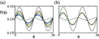
Figure 1: Steady distribution function of Stuart-Landau oscillators driven by Ornstein-Uhlenbeck processes when $\bm{G}=(1,0)$, $\sigma=0.3$, $\Omega=1$ and $c=0.1$. Symbols are numerical results and solid lines are theoretical predictions, Eq. (13). Dotted and dashed lines are Eq. (13) with $k=0$ and $k=\infty$ respectively. (a) $(\tau_{\eta},\tau_{\rho})=(0.2,0.1)$ (triangles), (0.1, 0.1) (circles) and (0.1, 0.2) (squares). (b) $(\tau_{\eta},\tau_{\rho})=(0.2,0.2)$ (triangles), (0.1, 0.1) (circles) and (0.05, 0.05) (squares).

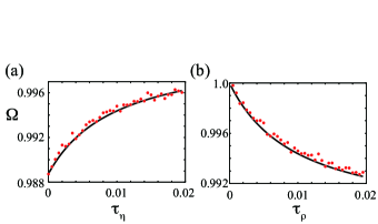
Figure 2: Mean frequency $\Omega$ of Stuart-Landau oscillators driven by Ornstein-Uhlenbeck processes when $\bm{G}=(x,0)$, $\sigma=0.3$, $\omega=1$ and $c=1$. Solid lines are theoretical predictions, Eq. (14). (a) $\tau_{\rho}=0.01$. (b) $\tau_{\eta}=0.01$.

References

- (1) Y. Kuramoto, Chemical Oscillation, Waves, and Turbulence (Springer-Verlag, Tokyo, 1984).
- (2) A. T. Winfree, The Geometry of Biological Time (Springer, New York, 2001), 2nd ed.
- (3) A. Pikovsky, M. Rosenblum, and J. Kurths, Synchronization: a universal concept in nonlinear sciences (Cambridge University Press, Cambridge, 2001).
- (4) B. Ermentrout, Neural. Compt. 8, 979, (1996).
- (5) J. A. Acebrón et al., Rev. Mod. Phys. 77, 137 (2005).
- (6) Y. Kawamura et al., Phys. Rev. Lett. 101, 024101 (2008).
- (7) G. B. Ermentrout, R. F. Galán, and N. N. Urban, Phys. Rev. Lett. 99, 248103 (2007).
- (8) J. Teramae and D. Tanaka, Phys. Rev. Lett. 93, 204103 (2004); Prog. Theor. Phys. Suppl. 161, 360 (2006).
- (9) D. Goldobin, M. Rosenblum, and A. Pikovsky, Phys. Rev. E 67, 061119 (2003). D. S. Goldobin and A. Pikovsky, Phys. Rev. E 71, 045201(R) (2005); Phys. Rev. E 73, 061906 (2006). D. S. Goldobin, Phys. Rev. E 78, 060104 (2008).
- (10) K. Nagai, H. Nakao, and Y. Tsubo, Phys. Rev. E 71, 036217 (2005); H. Nakao et al., Phys. Rev. E 72, 026220 (2005); H. Nakao, K. Arai, and Y. Kawamura, Phys. Rev. Lett. 98, 184101 (2007).
- (11) R. F. Galán, G. B. Ermentrout, and N. N. Urban, Phys. Rev. E. 76, 056110 (2007).
- (12) G. B. Ermentrout, R. F. Galán, and N. N. Urban, Trends neurosci. 31, 428 (2008).
- (13) J. Teramae and T. Fukai, Phys. Rev. Lett. 101, 248105 (2008).
- (14) K. K. Lin, E. Shea-Brown, and L. S. Young, arXiv:0805.3523v1 [q-bio.NC] (2008).
- (15) K. Yoshimura, K. Arai, Phys. Rev. Lett. 101, 154101 (2008).
- (16) H. Nakao, J. Teramae, and G. B. Ermentrout, arXiv:0812.3205v1 [nlin.AO] (2008).
- (17) N. G. van Kampen, Stochastic Processes in Physics and Chemistry (North-Holland, Amsterdam, 1981).
- (18) W. Horsthemke and R. Lefever, Noise-induced Transitions (Springer-Verlag, Berlin, 1984).
- (19) C. W. Gardiner, Handbook of Stochastic Methods (Springer-Verlag, Berlin, 1986).
- (20) L. Arnold, Random Dynamical systems (Springer, Berlin, 1998).
- (21) R. Kupferman, G. A. Pavliotis and A. M. Stuart, Phys. Rev. E 70, 036120 (2004).