Soft Constraints for Quality Aspects in Service Oriented Architectures

Abstract

We propose the use of Soft Constraints as a natural way to model Service Oriented Architecture. In the framework, constraints are used to model components and connectors and constraint aggregation is used to represent their interactions. The “quality of a service” is measured and considered when performing queries to service providers. Some examples consist in the levels of cost, performance and availability required by clients. In our framework, the QoS scores are represented by the softness level of the constraint and the measure of complex (web) services is computed by combining the levels of the components.

1 Introduction

Constraint programming is a powerful paradigm for solving combinatorial search problems that draws on a wide range of techniques from artificial intelligence, computer science, databases, programming languages, and operations research [10, 3, 26]. It is currently applied with success to many domains, such as scheduling, planning, vehicle routing, configuration, networks, and bioinformatics. The basic idea in constraint programming is that the user states the constraints and a general purpose constraint solver solves them. Constraints are just relations, and a Constraint Satisfaction Problem (CSP) states which relations should hold among the given decision variables (we refer to this classical view as “crisp” constraints). Constraint solvers take a real-world problem, represented in terms of decision variables and constraints, and find an assignment of values to all the variables that satisfies all the constraints.

Rather than trying to satisfy a set of constraints, sometimes people want to optimize them. This means that there is an objective function that tells us the quality of each solution, and the aim is to find a solution with optimal quality. For example, fuzzy constraints [10, 3, 26] allow for the whole range of satisfiability levels between $0$ and $1$. In weighted constraints, instead, each constraint is given a weight, and the aim is to find a solution for which the sum of the weights of the satisfied constraints is maximal.

The idea of the semiring-based formalism [10, 3] was to further extend the classical constraint notion, and to do it with a formalism that could encompass most of the existing extensions, as well as other ones not yet defined, with the aim to provide a single environment where properties could be proven once and for all, and inherited by all the instances. At the technical level, this was done by adding to the usual notion of a CSP the concept of a structure representing the levels of satisfiability of the constraints. Such a structure is a set with two operations (see Sec. 2 for further details): one (written $+$) is used to generate an ordering over the levels, while the other one ($\times$) is used to define how two levels can be combined and which level is the result of such combination. Because of the properties required on such operations, this structure is similar to a semiring (see Sec. 2): from here the terminology of “semiring-based soft constraint” [10, 3] (and Sec. 2), that is, constraints with several levels of satisfiability, and whose levels are (totally or partially) ordered according to the semiring structure. In general, problems defined according to the semiring-based framework are called Soft Constraint Satisfaction Problems (SCSPs).

The aim of this paper is to apply Quality of Service (QoS) measures for Service Oriented Architectures (SOAs) [25, 24]. Such architecture outlines a way of reorganizing software applications and infrastructure into a set of interacting services and aims at a loose coupling of services with operating systems, programming languages and other technologies. A SOA separates functions into distinct units or services, and these services communicate with each other by passing data from one service to another, or by coordinating an activity between two or more services. Web services [22, 2] can implement a service-oriented architecture.

SOAs clearly represent a distributed environment and QoS aspects become very important to evaluate, since the final integrated service must fulfill the non-functional requirements of the final users; this composition needs to be monitored [25, 24]. We are also interested in representing contracts and Service Level Agreements [2, 22] (SLAs) in terms of constraint based languages. The notions of contract and SLAs are very important in SOC since they allow to describe the mutual interactions between communicating parties and to express properties related to the quality of service such as cost, performance, reliability and availability. The existing languages for describing Web services (e.g. WSDL, WS-CDL and WS-BPEL) are not adequate for describing contracts and SLAs and, so far, there exists no agreement on a specific proposal in this sense: a general, established theory of contracts is still missing [2, 22].

The key idea of this paper is to use the a soft constraint framework in order to be able to manage SOAs in a declarative fashion by considering together both the requirements/interfaces of each service and their QoS estimation [31, 28, 29]. C-semirings can represent several QoS attributes, while soft constraints represent the specification of each service to integrate: they link these measures to the resources spent in providing it, for instance, “the reliability is equal to 80% plus 5% for each other processor used to execute the service”. This statement can be easily represented with a soft constraint where the number of processors corresponds to the $x$ variable, and the preference (i.e. reliability) level is given by the $5x+80$ polynomial.

Beside expressivity reasons, other advantages w.r.t. crisp constraints are that soft constraints can solve over-constrained problems (i.e. when it is not possible to solve all of them at the same time) and that, when we have to deal with quality, many related concepts are “smooth”: quality can be represented with intervals of “more or less” acceptable values. It has been proved that constraint in general are a powerful paradigm for solving combinatorial search problems [10, 3, 26]. Moreover, there exists a wide body of existing research results on solving (soft) CSP for large systems of constraints in a fully mechanized manner [10, 3].

The paper is organized as follows: Sec. 2 presents the minimum background notions needed to understand soft constraints, while Sec. 3 closes the introductory part by defining SOAs, QoS aspects and by showing how semiring instantiations can represent these non-functional aspects. Sec. 4 shows that the use of soft constraints permits us to perform a quantitative analysis of system integrity. Section 5 shows how QoS can be modeled and checked by using a soft constraint-based formal language. Finally, Sec. 6 present the related work, while Sec. 7 draws the final conclusions and discusses the directions for future work.

2 Background on Soft Constraints

Absorptive Semiring.

An absorptive semiring [6] $S$ can be represented as a $\langle A,+,\times,{\mathbf{0}},{\mathbf{1}}\rangle$ tuple such that: i) $A$ is a set and ${\mathbf{0}},{\mathbf{1}}\in A$; ii) $+$ is commutative, associative and ${\mathbf{0}}$ is its unit element; iii) $\times$ is associative, distributes over $+$, ${\mathbf{1}}$ is its unit element and ${\mathbf{0}}$ is its absorbing element. Moreover, $+$ is idempotent, ${\mathbf{1}}$ is its absorbing element and $\times$ is commutative. Let us consider the relation $\leq_{S}$ over $A$ such that $a\leq_{S}b$ iff $a+b=b$. Then it is possible to prove that (see [7]): i) $\leq_{S}$ is a partial order; ii) $+$ and $\times$ are monotonic on $\leq_{S}$; iii) ${\mathbf{0}}$ is its minimum and ${\mathbf{1}}$ its maximum; iv) $\langle A,\leq_{S}\rangle$ is a complete lattice and, for all $a,b\in A$, $a+b=lub(a,b)$ (where $lub$ is the least upper bound). Informally, the relation $\leq_{S}$ gives us a way to compare semiring values and constraints. In fact, when we have $a\leq_{S}b$ (or simply $a\leq b$ when the semiring will be clear from the context), we will say that b is better than a.

In [6] the authors extended the semiring structure by adding the notion of division, i.e. $\div$, as a weak inverse operation of $\times$. An absorptive semiring $S$ is invertible if, for all the elements $a,b\in A$ such that $a\leq b$, there exists an element $c\in A$ such that $b\times c=a$ [6]. If $S$ is absorptive and invertible, then, $S$ is invertible by residuation if the set $\{x\in A\mid b\times x=a\}$ admits a maximum for all elements $a,b\in A$ such that $a\leq b$ [6]. Moreover, if $S$ is absorptive, then it is residuated if the set $\{x\in A\mid b\times x\leq a\}$ admits a maximum for all elements $a,b\in A$, denoted $a\div b$. With an abuse of notation, the maximal element among solutions is denoted $a\div b$. This choice is not ambiguous: if an absorptive semiring is invertible and residuated, then it is also invertible by residuation, and the two definitions yield the same value.

To use these properties, in [6] it is stated that if we have an absorptive and complete semiring, then it is residuated. For this reason, since all classical soft constraint instances (i.e. Classical CSPs, Fuzzy CSPs, Probabilistic CSPs and Weighted CSPs) are complete and consequently residuated, the notion of semiring division (i.e. $\div$) can be applied to all of them.

Soft Constraint System.

A soft constraint [7, 3] may be seen as a constraint where each instantiation of its variables has an associated preference. Given $S=\langle A,+,\times,{\mathbf{0}},{\mathbf{1}}\rangle$ and an ordered set of variables $V$ over a finite domain $D$, a soft constraint is a function which, given an assignment $\eta:V\rightarrow D$ of the variables, returns a value of the semiring. Using this notation ${\mathcal{C}}=\eta\rightarrow A$ is the set of all possible constraints that can be built starting from $S$, $D$ and $V$.

Any function in ${\mathcal{C}}$ involves all the variables in $V$, but we impose that it depends on the assignment of only a finite subset of them. So, for instance, a binary constraint $c_{x,y}$ over variables $x$ and $y$, is a function $c_{x,y}:(V\rightarrow D)\rightarrow A$, but it depends only on the assignment of variables $\{x,y\}\subseteq V$ (the support of the constraint, or scope). Note that $c\eta[v:=d_{1}]$ means $c\eta^{\prime}$ where $\eta^{\prime}$ is $\eta$ modified with the assignment $v:=d_{1}$. Notice also that, with $c\eta$, the result we obtain is a semiring value, i.e. $c\eta=a$.

Given set ${\mathcal{C}}$, the combination function $\otimes:{\mathcal{C}}\times{\mathcal{C}}\rightarrow{\mathcal{C}}$ is defined as $(c_{1}\otimes c_{2})\eta=c_{1}\eta\times c_{2}\eta$ (see also [7, 3, 9]). Having defined the operation $\div$ on semirings, the constraint division function ${\ominus\div}:{\mathcal{C}}\times{\mathcal{C}}\rightarrow{\mathcal{C}}$ is instead defined as $(c_{1}\,{\ominus\div}\,c_{2})\eta=c_{1}\eta\div c_{2}\eta$ [6]. Informally, performing the $\otimes$ or the ${\ominus\div}$ between two constraints means building a new constraint whose support involves all the variables of the original ones, and which associates with each tuple of domain values for such variables a semiring element which is obtained by multiplying or, respectively, dividing the elements associated by the original constraints to the appropriate sub-tuples. The partial order $\leq_{S}$ over ${\mathcal{C}}$ can be easily extended among constraints by defining $c_{1}\sqsubseteq c_{2}\iff c_{1}\eta\leq c_{2}\eta$. Consider set ${\mathcal{C}}$ and partial order $\sqsubseteq$. Then an entailment relation $\vdash\subseteq\wp({\mathcal{C}})\times{\mathcal{C}}$ is defined s.t. for each $C\in\wp({\mathcal{C}})$ and $c\in{\mathcal{C}}$, we have $C\vdash c\iff\bigotimes C\sqsubseteq c$ (see also [3, 9]).

Given a constraint $c\in{\mathcal{C}}$ and a variable $v\in V$, the projection [7, 3, 9] of $c$ over $V\backslash\{v\}$, written $c\Downarrow_{(V\backslash\{v\})}$ is the constraint $c^{\prime}$ s.t. $c^{\prime}\eta=\sum_{d\in D}c\eta[v:=d]$. Informally, projecting means eliminating some variables from the support. This is done by associating with each tuple over the remaining variables a semiring element which is the sum of the elements associated by the original constraint to all the extensions of this tuple over the eliminated variables. To treat the hiding operator of the language, a general notion of existential quantifier is introduced by using notions similar to those used in cylindric algebras. For each $x\in V$, the hiding function [3, 9] is defined as $(\exists_{x}c)\eta=\sum_{d_{i}\in D}c\eta[x:=d_{i}]$.

To model parameter passing, for each $x,y\in V$ a diagonal constraint [3, 9] is defined as $d_{xy}\in{\mathcal{C}}$ s.t., $d_{xy}\eta[x:=a,y:=b]={\mathbf{1}}$ if $a=b$ and $d_{xy}\eta[x:=a,y:=b]={\mathbf{0}}$ if $a\neq b$. Considering a semiring $S=\langle A,+,\times,{\mathbf{0}},{\mathbf{1}}\rangle$, a domain of the variables $D$, an ordered set of variables $V$ and the corresponding structure ${\mathcal{C}}$, then $S_{C}=\langle{\mathcal{C}},\otimes,\bar{{\mathbf{0}}},\bar{{\mathbf{1}}},\exists_{x},d_{xy}\rangle$ is a cylindric constraint system (“a la Saraswat” [9]).

Soft CSP and an Example.

A Soft Constraint Satisfaction Problem (SCSP) [3] defined as $P=\langle C,con\rangle$: $C$ is the set of constraints and $con\subseteq V$ is the set of variables of interest for the constraint set $C$, which however may concern also variables not in $con$. This is called the best level of consistency and it is defined by $blevel(P)=Sol(P)\Downarrow_{\emptyset}$, where $Sol(P)=(\bigotimes C)\Downarrow_{con}$; notice that $supp(blevel(P))=\emptyset$. We also say that: $P$ is $\alpha$-consistent if $blevel(P)=\alpha$; $P$ is consistent iff there exists $\alpha>_{S}{\mathbf{0}}$ such that $P$ is $\alpha$-consistent; $P$ is inconsistent if it is not consistent.

Figure 1 shows a weighted CSP as a graph. Variables and constraints are represented respectively by nodes and by undirected arcs (unary for $c_{1}$ and $c_{3}$, and binary for $c_{2}$), and semiring values are written to the right of each tuple. The variables of interest (that is the set $con$) are represented with a double circle (i.e. variable $X$). Here we assume that the domain of the variables contains only elements $a$ and $b$. For example, the solution of the weighted CSP of Fig. 1 associates a semiring element to every domain value of variable $X$. Such an element is obtained by first combining all the constraints together. For instance, for the tuple $\langle a,a\rangle$ (that is, $X=Y=a$), we have to compute the sum of $1$ (which is the value assigned to $X=a$ in constraint $c_{1}$), $5$ (which is the value assigned to $\langle X=a,Y=a\rangle$ in $c_{2}$) and $5$ (which is the value for $Y=a$ in $c_{3}$). Hence, the resulting value for this tuple is $11$. We can do the same work for tuple $\langle a,b\rangle\rightarrow 7$, $\langle b,a\rangle\rightarrow 16$ and $\langle b,b\rangle\rightarrow 16$. The obtained tuples are then projected over variable x, obtaining the solution $\langle a\rangle\rightarrow 7$ and $\langle b\rangle\rightarrow 16$. The blevel for the example in Fig. 1 is $7$ (related to the solution $X=a$, $Y=b$).

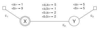
Figure 1: A soft CSP based on a Weighted semiring.

3 Service Oriented Architectures and QoS Aspects

Service Oriented Architecture (SOA) can be defined as a group of services, which communicate with each other [25, 24]. The process of communication involves either simple data passing or it could involve two or more services coordinating some activity. Basic services, their descriptions, and basic operations (publication, discovery, selection, and binding) that produce or utilize such descriptions constitute the SOA foundation. The main part of SOA is loose coupling of the components for integration. Services are defined by their interface, describing both functional and non-functional behaviour. Functional includes describing data formats, pre and post conditions and the operation performed by the service. Non-functional behaviour includes security and other QoS parameters. The main four features of SOA consist in Coordination, Monitoring, Conformance and Quality of Service (QoS) composition [25].

Services are self describing, open components that support rapid, low-cost composition of distributed applications. Services are offered by service providers, which are organizations that procure the service implementations, supply their service descriptions, and provide related technical and business support. Since services may be offered by different enterprises and communicate over the Internet, they provide a distributed computing infrastructure for both intra and cross-enterprise [2] application integration and collaboration. Service descriptions are used to advertise the service capabilities, interface, behaviour, and quality. Publication of such information, about available services, provides the necessary means for discovery, selection, binding, and composition of services. Service clients (end-user organizations that use some service) and service aggregators (organizations that consolidate multiple services into a new, single service offering) utilize service descriptions to achieve their objectives.

QoS measures include also dependability aspects: dependability as applied to a computer system is defined by the IFIP 10.4 Working Group on Dependable Computing and Fault Tolerance as [21]: “[..] the trustworthiness of a computing system which allows reliance to be justifiably placed on the service it delivers [..]”.

Some different QoS/dependability measurements can be applied to a system to determine its overall quality. A very general list of attributes is: i) Availability - the probability that a service is present and ready for use; ii) Reliability - the capability of maintaining the service and service quality; iii) Safety - the absence of catastrophic consequences; iv) Confidentiality - information is accessible only to those authorized to use it; v) Integrity - the absence of improper system alterations; and vi) Maintainability - to undergo modifications and repairs. Some of these attributes, as availability, are quantifiable by direct measurements (i.e. they are rather objective scores), but others are more subjective, e.g. safety.

The semiring algebraic structures (see Sec. 2) prove to be an appropriate and very expressive cost model to represent the QoS metrics shown in this Section. The cartesian product of multiple c-semirings is still a c-semiring [3] and, therefore, we can model also a multicriteria optimization. In the following list we present some possible semiring instantiations and some of the possible metrics they can represent:

• Weighted semirings $\langle\mathbb{R}^{+},min,\hat{+},\infty,0\rangle$ ($\hat{+}$ is the arithmetic sum). In general, this semiring can represent additive metrics: it can be used to count events or quantities to minimize the resulting sum, e.g. to save money while composing different services with different costs, or to minimize the downtime of service components (availability and reliability can be modeled this way).

• Fuzzy semirings $\langle[0,1],max,min,0,1\rangle$. It can be used to represent fuzzy preferences on components, e.g. low, medium or high reliability when detailed information is not available. This semiring can be used to represent concave metrics, in which the composition result of all the values is obtained by “flattening” to the “worst” or “best” value. One more application example is represented by the aggregation of bandwidth values along a network route or, however, by aggregating concave values on a pipeline of sub-services.

• Probabilistic semirings $\langle[0,1],max,\times,0,1\rangle$ ($\hat{\times}$ is the arithmetic multiplication). Multiplicative metrics can be modeled with this semiring. As an example, this semiring can optimize (i.e. maximize) the probability of successful behavior of services, by choosing the composition that optimizes the multiplication of probabilities. For example, the frequency of system faults can be studied from a probabilistic point of view; also availability can be represented with a percentage value.

• Set-Based semirings $\langle\mathcal{P}(A),\cup,\cap,\emptyset,A\rangle$. Properties and features of the service components can be represented with this semiring. For example, in order to represent related security rights, or time slots in which the services can be used (security issues).

• Classical semirings $\langle\{0,1\},\vee,\wedge,0,1\rangle$. The classical semiring can be adopted to cast crisp constraints in the semiring-based framework defined in [3, 8]. Even this semiring can be used to check if some properties are entailed by a service definition (i.e. true of false values), by composing the properties of its components together.

4 Soft Constraints to Enforce System Integrity

In this Section we show that soft constraints can model the implementation of a service described with a policy document [2, 22]; this really happens in practice by using the Web Services Description Language (WSDL) that is an XML-based language that provides a model for describing web services [22]. Moreover, by using the projection operator (i.e. $\Downarrow$ in Sec. 2) on this policy, which consists in the composition (i.e. $\otimes$ in Sec. 2) of different soft constraints, we obtain the external interface of the service that are used to match the requests. This view can be used to check the integrity of the system, that is if a particular service ensures the consistency of actions, values, methods, measures and principles; as a reminder, integrity can be seen as one of the QoS attributes proposed in Sec. 3. The integrity attribute is very important when different sub-services from distinct providers are composed together to offer a single structured service. The results presented here are inspired by the work in [4].

For the scenario example in Fig. 2, suppose to have a digital photo editing service decomposed as a set of sub-services; the compression/decompression module (i.e. COMPF) is located on the client side, while the other filter modules are located on the side of the editing company and can be reached through the network. The first module, i.e. BWF turns the colors in grey scale and the REDF filter absorbs green and blue and let only red become lighter. The client wants to compress (e.g. in a JPEG format) and send a remarkable number of photos (e.g. the client is a photo shop) to be double filtered and returned by the provider company; filters must be applied in a pipeline scheme, i.e. REDF goes after BWF.

The structure of the system represented in Fig. 2 corresponds to a federated system. It is defined as a system composed of components within different administrative entities cooperating to provide a service [2]; this definition perfectly matches our idea of SOA.

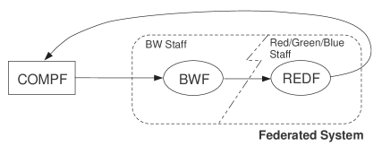
Figure 2: A federated photo editing system.

As a first example we consider the Classical semiring presented in Sec. 3, therefore, in practice we show a crisp constraint case. We suppose to have four variables outcomp, incomp, bwbyte and redbyte, which respectively represent the size in bytes of the photo at the beginning of the process, after applying the black-and-white filter, the red filter and after compressing the obtained black-and-white photo. Since the client has a limited memory space, it wants that the memory occupied by the photo does not increase after the filtering and compressing process:

$$\mbox{\sf{Memory}}\equiv\mbox{\sf{incomp}}\leq\mbox{\sf{outcomp}}$$

The following three constraints represent the policies compiled respectively by the staff of the BWF module, the REDF module and COMPF module. They state, following their order, that applying the BWF filter reduces the size of the image, applying the REDF filter reduces the size of the received black-and-white image and, at last, compressing the image reduces its size.

$$\mbox{\sf{BWFilter}}\equiv\mbox{\sf{bwbyte}}\leq\mbox{\sf{outcomp}}$$

$$\mbox{\sf{REDFilter}}\equiv\mbox{\sf{redbyte}}\leq\mbox{\sf{bwbyte}}$$

$$\mbox{\sf{Compression}}\equiv\mbox{\sf{incomp}}\leq\mbox{\sf{redbyte}}$$

The integration of the three policies (i.e. soft constraints) describes

$$\mbox{\sf{Imp1}}\equiv\mbox{\sf{BWFilter}}\otimes\mbox{\sf{RedFilter}}\otimes\mbox{\sf{Compression}}$$

Integrity is ensured in this system since Imp1 ensures the high-level requirement Memory.

$$\mbox{\sf{Imp1}}_{\Downarrow\{{\sf incomp},{\sf outcomp}\}}\sqsubseteq\mbox{\sf{Memory}}$$

We are unconcerned about the possible values of the ‘internal’ variables bwbyte and redbyte and thus the constraint relation $\mbox{\sf{Imp1}}_{\Downarrow\{{\sf incomp},{\sf outcomp}\}}$ describes the constraints in Imp1 that exist between variables incomp and outcomp}. By definition, the above equation defines that all of the possible solutions of $\mbox{\sf{Imp1}}_{\Downarrow\{{\sf incomp},{\sf outcomp}\}}$ are solutions of Memory, that is, for any assignment $\eta$ of variables then

$$\mbox{\sf{Imp1}}_{\Downarrow\{{\sf incomp},{\sf outcomp}\}}~{}{\eta}\leq_{S}\mbox{\sf{Memory}}~{}{\eta}$$

Definition 4.1

We say that the requirement $S$ locally refines requirement $R$ through the interface described by the set of variables $V$ iff $S_{\Downarrow V}\sqsubseteq R_{\Downarrow V}$.

Continuing the example in Fig. 2, we assume that the application system will behave reliably and uphold BWFilter and Compression. Let us suppose instead that it is not reasonable to assume that REDF will always act reliably, for example because the software of the red filter has a small bug when the size of the photo is $666$Kbyte. In practice, REDF could take on any behavior:

$$\overline{\mbox{\sf{RedFilter}}} \equiv (\mbox{\sf{redbyte}}\leq\mbox{\sf{bwbyte}}\vee\mbox{\sf{redbyte}}>\mbox{\sf{bwbyte}})=true$$

Imp2 $$\equiv \mbox{\sf{BWFilter}}\otimes\mbox{$\overline{\mbox{\sf{RedFilter}}}$}\otimes\mbox{\sf{Compression}}$$

Imp2 is a more realistic representation of the actual filtering process. It more accurately reflects the reliability of its infrastructure than the previous design Imp1. However, since redbyte is no longer constrained it can take on any value, and therefore, incomp is unconstrained and we have

$$\mbox{\sf{Imp2}}_{\Downarrow\{{\sf incomp},{\sf outcomp}\}}\not\sqsubseteq\mbox{\sf{Memory}}$$

that is, the implementation of the system is not sufficiently robust to be able to deal with internal failures in a safe way and uphold the memory probity requirement.

In [17, 18] the author argues that this notion of dependability may be viewed as a class of refinement whereby the nature of the reliability of the system is explicitly specified.

Definition 4.2

(Dependability and Constraints [4]) If $R$ gives requirements for an enterprise and $S$ is its proposed implementation, including details about the nature of the reliability of its infrastructure, then $S$ is as dependably safe as $R$ at interface that is described by the set of variables $E$ if and only if $S_{\Downarrow E}\sqsubseteq R_{\Downarrow E}$.

Quantitative analysis.

When a quantitative analysis of the system is required, then it is necessary to represent these properties using soft constraints. This can be done by simply considering a different semiring (see Sec. 3), while the same considerations provided for the previous example with crisp constraints (by using the Classical semiring) still hold.

With a quantitative analysis, now consider that we aim not only to have a correct implementation, but, if possible, to have the “best” possible implementation. We keep the photo editing example provided in Fig. 2, but we now represent the fact that constraints describe the reliability percentage, intended as the probability that a module will perform its intended function. For example, the following (probabilistic) soft constraint $c_{1}:\{\mbox{\sf{outcomp}},\mbox{\sf{bwbyte}}\}\rightarrow\mathbb{N}\rightarrow[0,1]$ shows how the compression reliability performed in BWFilter is linked to the initial and final number of bytes of the treated image:

$c_{1}(\mbox{\sf{outcomp}},\mbox{\sf{bwbyte}})=\begin{cases}1&\text{if $\mbox{\sf{outcomp}}\leq 1024Kb$},\\ 0&\text{if $\mbox{\sf{outcomp}}>4096Kb$},\\ 1-\frac{\mbox{\sf{outcomp}}}{100\;\;\cdot\;\;\mbox{\sf{bwbyte}}}&\text{otherwise}.\\ \end{cases}$

$c_{1}$ tells us that the compression does not work if the input image is more than $4Mb$, while is completely reliable if is less than $1Mb$. Otherwise, this probability depends on the compression efficiency: more that the image size is reduced during the compression, more that it is possible to experience some errors, and the reliability consequently decreases. For example, considering the definition of $c_{1}$, if the input image is $4096Kb$ and compressed is $1024Kb$, then the probability associated to this variable instantiation is $0.96$.

In the same way, we can define $c_{2}$ and $c_{3}$ that respectively shows the reliability for the REDFilter and Compression modules. Their composition $\mbox{\sf{Imp3}}=c_{1}\otimes c_{2}\otimes c_{3}$ represents the global reliability of the system. If $\mbox{\sf{Memory}}_{Prob}$ is the soft constraint representing the minimum reliability that the system must provide (e.g. $\mbox{\sf{Memory}}_{Prob}$ is expressed by a client of the photo editing system), then if

$$\mbox{\sf{Memory}}\sqsubseteq\mbox{\sf{Imp3}}$$

we are sure that the reliability requirements are entailed by our system. Moreover, by exploiting the notion of best level of consistency (see the blevel in Sec. 2), we can find the best (i.e. the most reliable) implementation among those possible.

At last, notice also that the projection operator (i.e. the $\Downarrow$ operator explained in Sec. 2) can be used to model a sort of function declaration to the “outside world”: soft constraints represent the internal implementation of the service, while projecting over some variables leads to the interface of the service, that is what is visible to the other software components.

5 A Nonmonotonic sccp Language for the Negotiation

In this Section we present a formal language based on soft constraints [11]; the language is tied to the monitoring of QoS aspects, as shown in Subsec. 5.1. Given a soft constraint system as defined in Sec. 2 and any related constraint $c$, the syntax of agents in nmsccp is given in Fig. 3. $P$ is the class of programs, $F$ is the class of sequences of procedure declarations (or clauses), $A$ is the class of agents, $c$ ranges over constraints, $X$ is a set of variables and $Y$ is a tuple of variables.

$P::=\>\>$	$F.A$
$F::=\>\>$	$p(Y)::A\mid F.F$
$A::=\>\>$	$success\mid tell(c)\rightarrowtail A\mid retract(c)\rightarrowtail A\mid update_{X}(c)\rightarrowtail A\mid E\mid A\|A\mid\exists x.A\mid p(Y)$
$E::=\>\>$	$ask(c)\rightarrowtail A\mid nask(c)\rightarrowtail A\mid E+E$

Figure 3: Syntax of the nmsccp language.

The $\rightarrowtail$ is a generic checked transition used by several actions of the language. Therefore, to simplify the rules in Fig. 5 we define a function $check_{\rightarrowtail}:\sigma\rightarrow\{true,false\}$ (where $\sigma\in{\mathcal{C}}$), that, parametrized with one of the four possible instances of $\rightarrowtail$ (C1-C4 in Fig. 4), returns true if the conditions defined by the specific instance of $\rightarrowtail$ are satisfied, or false otherwise. The conditions between parentheses in Fig. 4 claim that the lower threshold of the interval clearly cannot be “better” than the upper one, otherwise the condition is intrinsically wrong.

In Fig. 4 C1 checks if the $\alpha$-consistency of the problem is between $a_{1}$ and $a_{2}$. In words, C1 states that we need at least a solution as good as $a_{1}$ entailed by the current store, but no solution better than $a_{2}$; therefore, we are sure that some solutions satisfy our needs, and none of these solutions is “too good”.

C1: $\rightarrowtail=\rightarrow_{a_{1}}^{a_{2}}$	$check(\sigma)_{\rightarrowtail}=true\>\text{if}$	$\begin{cases}\sigma\Downarrow_{\emptyset}\not>_{S}a_{2}\\ \sigma\Downarrow_{\emptyset}\not<_{S}a_{1}\end{cases}$
	(with $a_{1}\not>a_{2}$)
C2: $\rightarrowtail=\rightarrow_{a_{1}}^{\phi_{2}}$	$check(\sigma)_{\rightarrowtail}=true\>\text{if}$	$\begin{cases}\sigma\not\sqsupset\phi_{2}\\ \sigma\Downarrow_{\emptyset}\not<_{S}a_{1}\end{cases}$
	(with $a_{1}\not>\phi_{2}\Downarrow_{\emptyset}$)

C3: $\rightarrowtail=\rightarrow_{\phi_{1}}^{a_{2}}$	$check(\sigma)_{\rightarrowtail}=true\>\text{if}$	$\begin{cases}\sigma\Downarrow_{\emptyset}\not>_{S}a_{2}\\ \sigma\not\sqsubset\phi_{1}\end{cases}$
	(with $\phi_{1}\Downarrow_{\emptyset}\not>a_{2}$)
C4: $\rightarrowtail=\rightarrow_{\phi_{1}}^{\phi_{2}}$	$check(\sigma)_{\rightarrowtail}=true\>\text{if}$	$\begin{cases}\sigma\not\sqsupset\phi_{2}\\ \sigma\not\sqsubset\phi_{1}\end{cases}$
	(with $\phi_{1}\not\sqsupset\phi_{2}$)

Otherwise, within the same conditions in parentheses, $check(\sigma)_{\rightarrowtail}=false$

Figure 4: Definition of the check function for each of the four checked transitions.

To give an operational semantics to our language we need to describe an appropriate transition system $\langle\Gamma,T,\rightarrow\rangle$, where $\Gamma$ is a set of possible configurations, $T\subseteq\Gamma$ is the set of terminal configurations and $\rightarrow\subseteq\Gamma\times\Gamma$ is a binary relation between configurations. The set of configurations is $\Gamma=\{\langle A,\sigma\rangle\}$, where $\sigma\in\mathcal{C}$ while the set of terminal configurations is instead $T=\{\langle success,\sigma\rangle\}$. The transition rules for the nmsccp language are defined in Fig. 5.

R1	$\frac{\displaystyle check(\sigma\otimes c)_{\rightarrowtail}}{\displaystyle\begin{array}[]{l}\langle\hbox{{\bf tell}}(c)\rightarrowtail A,\sigma\rangle\longrightarrow\langle A,\sigma\otimes c\rangle\end{array}}$	Tell
R2	$\frac{\displaystyle\sigma\vdash c\ \ \ \ \ check(\sigma)_{\rightarrowtail}}{\displaystyle\begin{array}[]{l}\langle\hbox{{\bf ask}}(c)\rightarrowtail A,\sigma\rangle\longrightarrow\langle A,\sigma\rangle\end{array}}$	Ask
R3	$\frac{\displaystyle\langle A,\sigma\rangle\longrightarrow\langle A^{\prime},\sigma^{\prime}\rangle}{\displaystyle\begin{array}[]{l}\langle A\parallel B,\sigma\rangle\longrightarrow\langle A^{\prime}\parallel B,\sigma^{\prime}\rangle\\ \langle B\parallel A,\sigma\rangle\longrightarrow\langle B\parallel A^{\prime},\sigma^{\prime}\rangle\end{array}}$	Parall1
R4	$\frac{\displaystyle\;\;\;\langle A,\sigma\rangle\longrightarrow\langle success,\sigma^{\prime}\rangle\;\;\;}{\displaystyle\begin{array}[]{l}\langle A\parallel B,\sigma\rangle\longrightarrow\langle B,\sigma^{\prime}\rangle\\ \langle B\parallel A,\sigma\rangle\longrightarrow\langle B,\sigma^{\prime}\rangle\end{array}}$	Parall2
R5	$\frac{\displaystyle\langle E_{j},\sigma\rangle\longrightarrow\langle A_{j},\sigma^{\prime}\rangle\ \ \ \ \ \ j\in[1,n]}{\displaystyle\begin{array}[]{l}\langle\Sigma_{i=1}^{n}E_{i},\sigma\rangle\longrightarrow\langle A_{j},\sigma^{\prime}\rangle\end{array}}$	Nondet

R6	$\frac{\displaystyle\sigma\not\vdash c\ \ \ \ \ \ check(\sigma)_{\rightarrowtail}}{\displaystyle\langle nask(c)\rightarrowtail A,\sigma\rangle\longrightarrow\langle A,\sigma\rangle}$	Nask
R7	$\frac{\displaystyle\sigma\sqsubseteq c\ \ \ \ \ \sigma^{\prime}=\sigma\,{\ominus\div}\,c\ \ \ \ \ check(\sigma^{\prime})_{\rightarrowtail}}{\displaystyle\langle retract(c)\rightarrowtail A,\sigma\rangle\longrightarrow\langle A,\sigma^{\prime}\rangle}$	Retract
R8	$\frac{\displaystyle\sigma^{\prime}=(\sigma\Downarrow_{(V\backslash X)})\otimes c\ \ \ \ \ check(\sigma^{\prime})_{\rightarrowtail}}{\displaystyle\langle update_{X}(c)\rightarrowtail A,\sigma\rangle\longrightarrow\langle A,\sigma^{\prime}\rangle}$	Update
R9	$\frac{\displaystyle\langle A[x/y],\sigma\rangle\longrightarrow\langle B,\sigma^{\prime}\rangle}{\displaystyle\langle\exists x.A,\sigma\rangle\longrightarrow\langle B,\sigma^{\prime}\rangle}\text{ with $y$ {\em fresh}}$	Hide
R10	$\frac{\displaystyle\langle A,\sigma\rangle\longrightarrow\langle B,\sigma^{\prime}\rangle}{\displaystyle\langle p(Y),\sigma\rangle\longrightarrow\langle B,\sigma^{\prime}\rangle}\ \ \ \ {\it p(Y)::A\in F}$	P-call

Figure 5: The transition system for nmsccp.

In the following we provide a description of the transition rules in Fig. 5. For further details, please refer to [11]. In the Tell rule (R1), if the store $\sigma\otimes c$ satisfies the conditions of the specific $\rightarrowtail$ transition of Fig. 4, then the agent evolves to the new agent $A$ over the store $\sigma\otimes c$. Therefore the constraint $c$ is added to the store $\sigma$. The conditions are checked on the (possible) next-step store: i.e. $check(\sigma^{\prime})_{\rightarrowtail}$. To apply the Ask rule (R2), we need to check if the current store $\sigma$ entails the constraint $c$ and also if the current store is consistent with respect to the lower and upper thresholds defined by the specific $\rightarrowtail$ transition arrow: i.e. if $check(\sigma)_{\rightarrowtail}$ is true.

Parallelism and nondeterminism: the composition operators $+$ and $\|$ respectively model nondeterminism and parallelism. A parallel agent (rules R3 and R4) will succeed when both agents succeed. This operator is modelled in terms of interleaving (as in the classical ccp): each time, the agent $A\parallel B$ can execute only one between the initial enabled actions of $A$ and $B$ (R3); a parallel agent will succeed if all the composing agents succeed (R4). The nondeterministic rule R5 chooses one of the agents whose guard succeeds, and clearly gives rise to global nondeterminism. The Nask rule is needed to infer the absence of a statement whenever it cannot be derived from the current state: the semantics in R6 shows that the rule is enabled when the consistency interval satisfies the current store (as for the ask), and $c$ is not entailed by the store: i.e. $\sigma\not\sqsubseteq c$. Retract: with R7 we are able to “remove” the constraint $c$ from the store $\sigma$, using the ${\ominus\div}$ constraint division function defined in Sec. 2. According to R7, we require that the constraint $c$ is entailed by the store, i.e. $\sigma\sqsubseteq c$. The semantics of Update rule (R8) [12] resembles the assignment operation in imperative programming languages: given an $update_{X}(c)$, for every $x\in X$ it removes the influence over $x$ of each constraint in which $x$ is involved, and finally a new constraint $c$ is added to the store. To remove the information concerning all $x\in X$, we project (see Sec. 2) the current store on $V\backslash X$, where $V$ is the set of all the variables of the problem and $X$ is a parameter of the rule (projecting means eliminating some variables). At last, the levels of consistency are checked on the obtained store, i.e. $check(\sigma^{\prime})_{\rightarrowtail}$. Notice that all the removals and the constraint addition are transactional, since are executed in the same rule. Hidden variables: the semantics of the existential quantifier in R9 can be described by using the notion of freshness of the new variable added to the store [11]. Procedure calls: the semantics of the procedure call (R10) has already been defined in [9]: the notion of diagonal constraints (as defined in Sec. 2) is used to model parameter passing.

5.1 Example

One application of the nmsccp language is to model generic entities negotiating a formal agreement, i.e. a SLA [2, 22], where the level of service is formally defined. The main task consists in accomplishing the requests of all the agents by satisfying their QoS requirements. Considering the fuzzy negotiation in Fig. 6 (Fuzzy semiring: $\langle[0,1],max,min,0,1\rangle$) both a provider and a client (offering and acquiring a web service, for example) can add their request to the store $\sigma$ (respectively $tell(c_{p})$ and $tell(c_{c})$): the thick line represents the consistency of $\sigma$ after the composition (i.e. $min$), and the blevel of this SCSP (see Sec. 2) is the max, where both requests intersects (i.e. in $0.5$).

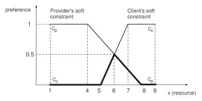
Figure 6: The graphical interpretation of a fuzzy agreement.

We present three short examples to suggest possible negotiation scenarios. We suppose there are two distinct companies (e.g. providers $P_{1}$ and $P_{2}$) that want to merge their services in a sort of pipeline, in order to offer to their clients a single structured service: e.g. $P_{1}$ completes the functionalities of $P_{2}$. This example models the cross-domain management of services proposed in [2]. The variable $x$ represents the global number of failures they can sustain during the service provision, while the preference models the number of hours (or a money cost in hundreds of euros) needed to manage them and recover from them. The preference interval on transition arrows models the fact that both $P_{1}$ and $P_{2}$ explicitly want to spend some time to manage the failures (the upper bound in Fig. 4), but not so much time (lower bound in Fig. 4). We will use the Weighted semiring and the soft constraints given in Fig. 7. Even if the examples are based on a single criterion (i.e. the number of hours) for sake of simplicity, they can be extended to the multicriteria case, where the preference is expressed as a tuple of incomparable criteria.

Example 5.1 (Tell and negotiation)

$P_{1}$ and $P_{2}$ both want to present their policy (respectively represented by $c_{4}$ and $c_{3}$) to the other party and to find a shared agreement on the service (i.e. a SLA). Their agent description is: $P_{1}\equiv\langle tell(c_{4})\rightarrow_{\infty}^{0}tell(s_{p2})\rightarrow_{\infty}^{0}ask(s_{p1})\rightarrow_{10}^{2}success\rangle||\langle tell(c_{3})\rightarrow_{\infty}^{0}tell(s_{p1})\rightarrow_{\infty}^{0}ask(s_{p2})\rightarrow_{4}^{1}success\rangle\equiv P_{2}$, executed in the store with empty support (i.e. $\bar{0}$). Variables $s_{p1}$ and $s_{p2}$ are used only for synchronization and thus will be ignored in the following considerations (e.g. replaced by the $SYNCHRO_{i}$ agents in Ex. 5.2). The final store (the merge of the two policies) is $\sigma=(c_{4}\otimes c_{3})\equiv 2x+x+5$, and since $\sigma\Downarrow_{\emptyset}=5$ is not included in the last preference interval of $P_{2}$ (between $1$ and $4$), $P_{2}$ does not succeed and a shared agreement cannot be found. The practical reason is that the failure management systems of $P_{1}$ need at least $5$ hours (i.e. $c_{4}=x+5$) even if no failures happen (i.e. $x=0$). Notice that the last interval of $P_{2}$ requires that at least $1$ hour is spent to check failures.

$$c_{1}:(\{x\}\rightarrow\mathbb{N})\rightarrow\mathbb{R}^{+}\;\;\text{ s.t. }c_{1}(x)=x+3\hskip 31.2982ptc_{2}:(\{y\}\rightarrow\mathbb{N})\rightarrow\mathbb{R}^{+}\,\,\text{s.t.}\;c_{2}(y)=y+1$$

$\ \,c_{3}:(\{x\}\rightarrow\mathbb{N})\rightarrow\mathbb{R}^{+}\;\;\text{ s.t. }c_{3}(x)=2x$             $c_{4}:(\{x\}\rightarrow\mathbb{N})\rightarrow\mathbb{R}^{+}\;\text{ s.t. }c_{4}(x)=x+5$

Figure 7: Four Weighted soft constraints.

Example 5.2 (Retract)

After some time (still considering Ex. 5.1), suppose that $P_{1}$ wants to relax the store, because its policy is changed: this change can be performed from an interactive console or by embedding timing mechanisms in the language as explained in [5]. The removal is accomplished by retracting $c_{1}$, which means that $P_{1}$ has improved its failure management systems. Notice that $c_{1}$ has not ever been added to the store before, so this retraction behaves as a relaxation; partial removal is clearly important in a negotiation process. $P_{1}\equiv\langle tell(c_{4})\rightarrow_{\infty}^{0}SYNCHRO_{P1}\rightarrow_{10}^{2}retract(c_{1})\rightarrow_{10}^{2}success\rangle||\langle tell(c_{3})\rightarrow_{\infty}^{0}SYNCHRO_{P2}\rightarrow_{4}^{1}success\rangle\equiv P_{2}$ is executed in $\bar{0}$. The final store is $\sigma=c_{4}\otimes c_{3}\,{\ominus\div}\,c_{1}\equiv 2x+2$, and since $\sigma\Downarrow_{\emptyset}=2$, both $P_{1}$ and $P_{2}$ now succeed (it is included in both intervals).

Example 5.3 (Update)

The update can instead be used for substantial changes of the policy: for example, suppose that $P_{1}\equiv\langle tell(c_{1})\rightarrow_{\infty}^{0}update_{\{x\}}(c_{2})\rightarrow_{\infty}^{0}success,\bar{0}\rangle$. This agent succeeds in the store $\bar{0}\otimes c_{1}\Downarrow_{(V\backslash\{x\})}\otimes c_{2}$, where $c_{1}\Downarrow_{(V\backslash\{x\})}=\bar{3}$ and $\bar{3}\otimes c_{2}\equiv y+4$ (i.e. the polynomial describing the final store). Therefore, the first policy based on the number of failures (i.e. $c_{1}$) is updated such that $x$ is “refreshed” and the newly added policy (i.e. $c_{2}$) depends only on the number $y$ of system reboots. The consistency level of the store (i.e. the number of hours) now depends only on the $y$ variable of the SCSP. Notice that the $\bar{3}$ component of the final store derives from the “old” $c_{1}$, meaning that some fixed management delays are included also in this new policy.

6 Related Work

There exist already several proposals for languages which allow to specify (Web) services and their composition, at different levels of abstractions, ranging from description languages such as WSDL (which allows to describe services essentially as collections of ports), to orchestration languages (XLANG, WSFL and WS-BPEL) and choreography languages (WS-CDL and BPEL4Chor) which allow to define composition of services either in terms of a centralized meta-service (the orchestrator) or by considering the reciprocal interactions (the choreography) among the different services (without centralization). There exist also some specific proposals [16, 14] for describing contracts and their relevant properties. However a general, established theory of contracts is still missing. Furthermore most languages do not take into account SLAs, that is aspects of contracts such as cost, performance or availability, which are related to QoS.

Other papers have been proposed in order to study dependability aspects in SOAs, for example by using the Architecture Analysis and Design Language (AADL). In [27] the authors purpose a modeling framework allowing the generation of dependability-oriented analytical models from AADL models, to facilitate the evaluation of dependability measures, such as reliability or availability. The AADL dependability model is transformed into a Generalized Stochastic Petri Net (GSPN) by applying model transformation rules.

The frameworks presented in this paper can join the other formal approaches for architectural notations: Graph-Based, Logic-Based and Process Algebraic approaches [13]. A formal foundation underlying is definitely important, since, for example, UML alone can offer a number of alternatives for representing architectures: therefore, this lack of precision can lead to a semantic misunderstanding of the described architectural model [20]. Compared to other formal methods [13], constraints are very expressive and close to the human way of describing properties and relationships; in addition, their solution techniques have a long and successful history [26]. The qualitative/quantitative architectural evaluation can be accomplished by considering different semirings (see Sec 2): our framework is highly parametric and can consequently deal with different QoS metrics, as long as they can be represented as semirings.

Other works have studied the problem of issuing requests to a composition of web services as a crisp constraint-based problem [23], but without optimizing non-functional aspects of services, as we instead do with (semiring-based) soft constraints. For a more precise survey on the architectural description of dependable software systems, please refer to [19]. The most direct comparison for nmsccp in Sec. 5 is with the work in [15], in which soft constraints are combined with a name-passing calculus. The most important difference is that in nmsccp we do not have the concept of constraint token and it is possible to remove every $c$ that is entailed by the store, even if $c$ is syntactically different from all the $c$ previously added.

7 Conclusions and Future Work

We have proved that soft constraints and their related operators (e.g. $\otimes$, ${\ominus\div}$, $\Downarrow$ in Sec. 2) can model and manage the composition of services in SOAs by taking in account QoS metrics. The key idea is that constraint relationships model the implementation of a service component (described as a policy), while the “softness” (i.e. the preference value associated with the soft constraint) represents one or more QoS measures, as reliability, availability and so on (see Sec. 3). In this way, the composition of services can be monitored and checked, and the best quality result can be found on this integration. It may also be desirable to describe constraints and capabilities (also, “policy”) regarding security: a web service specification could require that, for example, “you MUST use HTTP Authentication and MAY use GZIP compression”.

Two different but very close contributions are collected in this work. The first contribution in Sec. 4 is that the use of soft constraints permits one to perform a quantitative analysis of system integrity. The second contribution, explained in Sec. 5, proposes the use of a formal language based on soft constraints in order to model the composition of different service components while monitoring QoS aspects at the same time.

All the models and techniques presented in this work can be implemented and integrated together in a suite of tools, in order to manage and monitor QoS while building SOAs. To accomplish this task, we could extend an existent solver such as Gecode [30], which is an open, free, portable, accessible, and efficient environment for developing constraint-based systems and applications. The main results would be the development of a SOA query engine, that would use the constraint satisfaction solver to select which available service will satisfy a given query. It would also look for complex services by composing together simpler service interfaces.

References

- [1]
- [2] P. Bhoj, S. Singhal & S. Chutani (2001): SLA management in federated environments. Comput. Networks 35(1), pp. 5–24.
- [3] S. Bistarelli (2004): Semirings for Soft Constraint Solving and Programming, LNCS 2962. Springer, London, UK.
- [4] S. Bistarelli & S.N. Foley (2003): A Constraint Framework for the Qualitative Analysis of Dependability Goals: Integrity. In: S. Anderson, M. Felici & B. Littlewood, editors: SAFECOMP, LNCS 2788. Springer, pp. 130–143.
- [5] S. Bistarelli, M. Gabbrielli, M. C. Meo & F. Santini (2008): Timed Soft Concurrent Constraint Programs. In: Doug Lea & Gianluigi Zavattaro, editors: COORDINATION, LNCS 5052. Springer, pp. 50–66.
- [6] S. Bistarelli & F. Gadducci (2006): Enhancing Constraints Manipulation in Semiring-Based Formalisms. In: European Conference on Artificial Intelligence (ECAI). pp. 63–67.
- [7] S. Bistarelli, U. Montanari & F. Rossi (1997): Semiring-based constraint satisfaction and optimization. J. ACM 44(2), pp. 201–236.
- [8] S. Bistarelli, U. Montanari & F. Rossi (1997): Semiring-based Constraint Solving and Optimization. Journal of the ACM 44(2), pp. 201–236.
- [9] S. Bistarelli, U. Montanari & F. Rossi (2006): Soft concurrent constraint programming. ACM Trans. Comput. Logic 7(3), pp. 563–589.
- [10] S. Bistarelli & F. Rossi (2008): Semiring-Based Soft Constraints. In: P. Degano, R. De Nicola & J. Meseguer, editors: Concurrency, Graphs and Models, LNCS 5065. Springer, pp. 155–173.
- [11] S. Bistarelli & F. Santini (2009): A Nonmonotonic Soft Concurrent Constraint Language for SLA Negotiation. In: A. Aldini, M.H. ter Beek & F. Gadducci, editors: VODCA’08: Proceedings 3rd International Workshop on Views On Designing Complex Architectures, Electr. Notes Theor. Comput. Sci. 236. pp. 147–162.
- [12] F. S. de Boer, J. N. Kok, C. Palamidessi & J. M. M. Rutten (1993): Non-monotonic Concurrent Constraint Programming. In: ILPS. pp. 315–334.
- [13] J.S. Bradbury, J.R. Cordy, J. Dingel & M. Wermelinger (2004): A survey of self-management in dynamic software architecture specifications. In: WOSS’04: Proceedings of the 1st ACM SIGSOFT workshop on Self-managed systems. ACM, New York, NY, USA, pp. 28–33.
- [14] M. Bravetti & G. Zavattaro (2007): Towards a Unifying Theory for Choreography Conformance and Contract Compliance. In: M. Lumpe & W. Vanderperren, editors: Software Composition, LNCS 4829. Springer, pp. 34–50.
- [15] M.G. Buscemi & U. Montanari (2007): CC-Pi: A Constraint-Based Language for Specifying Service Level Agreements. In: ESOP’07, LNCS 4421. Springer, pp. 18–32.
- [16] S. Carpineti, G. Castagna, C. Laneve & L. Padovani (2006): A Formal Account of Contracts for Web Services. In: Mario Bravetti, Manuel Núñez & Gianluigi Zavattaro, editors: WS-FM, LNCS 4184. Springer, pp. 148–162.
- [17] S.N. Foley (1998): Evaluating system integrity. In: NSPW ’98: Proceedings of the 1998 workshop on New security paradigms. ACM, New York, NY, USA, pp. 40–47.
- [18] S.N. Foley (2003): A Non-Functional Approach to System Integrity. In: IEEE Journal on Selected Areas in Commications, 21(1). pp. 36–43.
- [19] C. Gacek & R. de Lemos (2006): Architectural Description of Dependable Software Systems. In: D. Besnard, C. Gacek & C. Jones, editors: Structure for Dependability: Computer-Based Systems from an Interdisciplinary Perspective. Springer-Verlag, pp. 127–142.
- [20] D. Garlan, S.-W. Cheng & A. J. Kompanek (2002): Reconciling the needs of architectural description with object-modeling notations. Sci. Comput. Program. 44(1), pp. 23–49.
- [21] IFIP (1998): IFIP WG 10.4 on Dependable Computing and Fault Tolerance. Technical Report, International Federation For Information Processing.
- [22] A. Keller & H. Ludwig (2003): The WSLA Framework: Specifying and Monitoring Service Level Agreements for Web Services. J. Netw. Syst. Manage. 11(1), pp. 57–81.
- [23] A. Lazovik, M. Aiello & R. Gennari (2005): Encoding Requests to Web Service Compositions as Constraints. In: Conference on Principles and Practice of Constraint Programming (CP’05). pp. 782–786.
- [24] M.P. Papazoglou (2003): Service-Oriented Computing: Concepts, Characteristics and Directions. Web Information Systems Engineering, International Conference on 0, p. 3.
- [25] M.P. Papazoglou & D. Georgakopoulos (2003): Service oriented computing. Commun. ACM 46(10).
- [26] F. Rossi, P. van Beek & T. Walsh (2006): Handbook of Constraint Programming (Foundations of Artificial Intelligence). Elsevier Science Inc., New York, NY, USA.
- [27] A.E. Rugina, K. Kanoun & M. Kaâniche (2006): A System Dependability Modeling Framework Using AADL and GSPNs. In: R. de Lemos, C. Gacek & A. B. Romanovsky, editors: WADS, LNCS 4615. Springer, pp. 14–38.
- [28] F. Santini (2008): Managing Quality of Service with Soft Constraints. In: D. Fox & C. P. Gomes, editors: AAAI. AAAI Press, pp. 1869–1870.
- [29] F. Santini (2008): Managing Quality of Service with Soft Constraints. In: M. G. de la Banda & E. Pontelli, editors: ICLP, LNCS 5366. Springer, pp. 815–817.
- [30] C. Schulte (2002): Programming Constraint Services, Lecture Notes in Artificial Intelligence 2302. Springer-Verlag.
- [31] M. Wirsing, A. Clark, S. Gilmore, M. Hölzl, A. Knapp, N. Koch & A. Schroeder (2006): Semantic-Based Development of Service-Oriented Systems. In: E. Najm, J.F. Pradat-Peyre & V. Donzeau-Gouge, editors: FORTE, LNCS 4229. Springer, pp. 24–45.