Bayesian Forecasting of WWW Traffic
on the Time Varying Poisson Model

Abstract

Traffic forecasting from past observed traffic data with small calculation complexity is one of important problems for planning of servers and networks. Focusing on World Wide Web (WWW) traffic as fundamental investigation, this paper would deal with Bayesian forecasting of network traffic on the time varying Poisson model from a viewpoint from statistical decision theory. Under this model, we would show that the estimated forecasting value is obtained by simple arithmetic calculation and expresses real WWW traffic well from both theoretical and empirical points of view.

Keywords: World Wide Web (WWW) traffic, traffic engineering, statistical decision theory, time varying Poisson distribution, long-range dependence (LRD)

1 Introduction

Under network environment such as Internet, planning of servers and networks is one of important problems for stable operation. It is often typical situation that administrators analyze logs on their servers and networks. They may frequently look into result of log analysis software where these tools usually have some functions to periodically summarize logs. For example, webalizer [Barrett] and analog [Turner] etc.  have been widely used among World Wide Web (WWW) server administrators or users for long years. These tools usually summarize the logs by counting hourly, daily, and monthly numbers of hits, files, and pages etc. Administrators would often make their operation plans with combination of their experience and intuition from these logs. In this case, traffic forecasting rule is not clearly formulated and those summarized logs remain in the field of descriptive statistics from the statistical point of view.

On the other hand, researchers in the field of traffic engineering have been suggesting a lot of analysis models. Probabilistic approach is one of viewpoints in this field. It is wide-spread fact that the stationary Poisson distribution is not always suitable for Internet traffic because of its nature of non-stationality [Paxon] [Karagiannis] and long-range dependence (LRD) [Leland] [Paxon] etc. Therefore desirable conditions of good traffic models are to have structures to express such nature at least. Furthermore, another requirement of models is to have a structure of traffic forecasting. For this point, parameter estimation is often performed at first under assumption of the stationarity [Scherrer], then the estimated parameter is substituted for the parameter of model. This approach has been wide-spread in the field of inferential statistics from the statistical point of view.

However, substituting the estimated parameter as a constant for the model’s parameter is not always suitable especially on forecasting problems. This is because there is often no guarantee that the assumptions under the parameter estimation of the model always hold for future unknown data set. Bayesian approach [Berger][Bernardo] is one of alternatives for this point. In Bayesian approach, a probability distribution of parameter is assumed as the prior distribution. If new data is observed, then the Bayes theorem updates the prior distribution of parameter to the posterior distribution and then forecasts the posterior distribution of data. Recently, this approach has been widely applied to many forecasting problems especially in the field of information technologies and bioinformatics etc. In order to take Bayesian approach, statistical decision theory is an important theoretical framework from the statistical point of view.

Taking the above factors into account, this paper would deal with Bayesian forecasting of WWW traffic on the non-stationary i.e. time varying Poisson model. Bayesian forecasting on time varying parameter model has been proposed in [Smith] by defining certain class of parameter transformation function. However, it has not yet been discussed about any predictive estimator nor definite transformation function of parameter [Smith]. This paper would clearly define a random-walking type of transformation function of parameter to obtain the Bayes optimal prediction for WWW traffic. Then its effectiveness would be evaluated with real WWW traffic data. In this model, time varying degree is caught by a real valued constant $k\,(0<k\leq 1)$ and this constant would play an important role throughout this paper. Another feature is that the traffic forecasting value is obtained by simple arithmetic calculations under known $k$. In general, the Bayes theorem often results in large calculation costs. However, certain combination of parameter distribution and its transformation function solves this problem. We believe that this point can be helpful not only for theoretical calculation cost but also for real implementation on WWW log analysis tools [Barrett] [Turner].

The rest of this paper is organized as the followings. Section 2 gives some definitions and explanations of the forecasting model with time varying Poisson distribution. Section LABEL:Simulation shows some analysis examples of real WWW traffic data to validate this paper’s approach and Section LABEL:Discussion gives their discussions. Finally, Section LABEL:Conclusion concludes this paper.

2 The Time Varying Poisson Model

2.1 Definitions

Suppose $X$ is a discrete random variable and $p(x)=Pr\{X=x\}$ is the probability distribution where real number $x$ is each element of space of $X$. Throughout this paper, the probability distribution of $X$ is assumed to depend on real valued parameter $\theta\in\Theta$. The true parameter $\theta^{*}\in\Theta$ is unknown, however, the probability distribution of parameter $p(\theta)$ is assumed to be known. Hereafter the probability distribution of $X$ under parameter $\theta$ is simply denoted as $p(x\bigm{|}\theta)$.

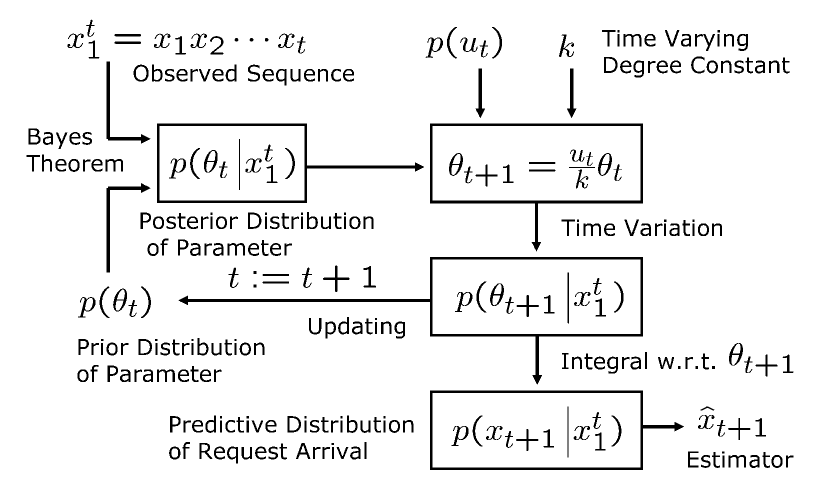
Figure 1: Overview of the inferential process.

Let $t=1,2,\cdots$ be discrete time and $x_{t}=0,1,\cdots$ be number of WWW request arrivals at time $t$, respectively. This paper focuses on $x_{t}$ for traffic analysis by assuming probability distribution $p(x_{t}\bigm{|}\theta_{t})$ where $\theta_{t}>0$ is a time varying density parameter at time $t$. The time varying Poisson model takes sequence of $x_{1}^{t}=x_{1}x_{2}\cdots x_{t}$ as input and calculates $\hat{x}_{t+1}$ as an output estimator where the prior distribution of parameter $p(\theta_{t})$ and time variation rule of $\theta_{t}$ are known. The overview of the inferential process is depicted in Figure 1.

In Figure 1, $x_{t}$ is assumed to be the Poisson distribution with a time varying density parameter $\theta_{t}$ as follows:

For $x_{t}=0,1,2,\cdots$, Cc p(x_t|θ_t) &= exp(-θt)xt!(θ_t)^x_t , where $\theta_{t}>0$ is a time varying density parameter.

For parameter $\theta_{t}$, the following time varying model is assumed:

For $\theta_{t+1},\theta_{t}>0$, Cc θ_t+1&=utkθ_t , where $k$ is a constant such that $0<k\leq 1$, and $0<u_{t}<1$ is a continuous random variable which is conditionally independent from $\theta_{t}$. (1) represents a transformation of $\theta_{t+1}$ from both $\theta_{t}$ and $u_{t}$ under a known constant $k$. This transformation is regarded as a kind of random-walk.

Furthermore, the initial random variables of $\theta_{1}$ and $u_{1}$ are from the Gamma and Beta distributions, respectively. The followings give their definitions:

For $\theta_{1}>0$, lL p(θ_1|α_1,β_1) &= (β1)α1Γ(α1)exp(-θ_1β_1)(θ_1)^(α_1)-1 , where $\alpha_{1}>0,\ \beta_{1}>0$ are parameters of the Gamma distribution.

In (1), $\Gamma\left(x\right)$ is the Gamma function defined below: Cc Γ(x) &= ∫^∞_0 y^x-1exp(-y)dy ,

where $x>0$.

For $0<u_{1}<1$, Ll $\displaystyle p\left(u_{1}|k\alpha_{1},\left(1-k\right)\alpha_{1}\right)$
&= Γ(α1)Γ​ (kα1)​ Γ[(1 ​ - ​ k )α1] ​ (u_1)^(kα_1)-1​ ( 1 ​ - ​ u_1)^[(1-k)α_1]-1 ,
where $k\alpha_{1}>0,\ \left(1-k\right)\alpha_{1}>0$ are parameters of the Beta distribution.

In (1) and (2.1), two random variables $\theta_{1}$ and $u_{1}$ have a real value $\alpha_{1}>0$ as their parameters in common. This means that $\theta_{1}$ and $u_{1}$ are conditionally independent.

Remarks 2.1

In (1), a constant $0<k\leq 1$ expresses time varying degree of $\theta_{t}$. If $k=1$, (1) simply becomes $\theta_{t+1}=u_{t}\theta_{t}$. In this case, $\theta_{t+1}$ does not vary since the variance of $u_{t}$ , which equals to $k(1-k)/(\alpha_{t}+1)$ according to the nature of Beta distribution, becomes zero. This means that the Poisson distribution of $x_{t}$ in (1) is stationary.

If $k<1$, on the other hand, $\theta_{t+1}$ varies depending on the previous $\theta_{t}$ which expresses the time varying Poisson model. If $k=0.5$, the time varying degree of $\theta_{t}$ becomes maximum since the variance of $u_{t}$ takes the maximum value. Thus the proposed model defined in (1)–(2.1) includes a classical stationary Poisson distribution as a special case if $k=1$. Moreover, $k$ plays another important role which would be explained in Remarks LABEL:remark2_of_model.

2.2 Updating Density Parameter $\theta_{t}$

As shown in Figure 1, the parameter updating rule from $\theta_{t}$ to $\theta_{t+1}$ consists of Bayes theorem and time variation. In the followings, this subsection 2.2 is divided into three parts. The first 2.2.1 describes the updating rule by Bayes theorem for $t\geq 2$, the second 2.2.2 describes the initial condition of the prior distribution $p\left(\theta_{1}\right)$ for $t=1$, and the last 2.2.3 describes general time variation rule which is mainly discussed in [Smith].

2.2.1 The Posterior Distribution of Density Parameter

Suppose that sequence $x_{1}^{t-1}$ is already observed where $t\geq 2$ and the prior distribution of parameter $p\left(\theta_{t}\bigm{|}\alpha_{t},\beta_{t},x_{1}^{t-1}\right)$ is defined as the Gamma distribution in (1) for $t\geq 2$. If new $x_{t}$ is observed, the posterior distribution of $p\left(\theta_{t}\bigm{|}x_{1}^{t}\right)$ by the Bayes theorem is obtained as the following: Ll $\displaystyle p\left(\theta_{t}\bigm{|}x_{1}^{t}\right)$
&= p(xt|θt)p(θt|αt,βt,x1t-1)∫0∞p(xt|θt)p(θt|αt,βt,x1t-1)dθt
= (βt​ + ​ 1 )αt+xtΓ(αt​ + ​ xt) ​ exp[-θ_t(β_t ​ + ​ 1)] ​ (θ_t)^(α_t+x_t)-1 , where $t\geq 2$.

(2.2.1) means that the posterior distribution $p\left(\theta_{t}\bigm{|}x_{1}^{t}\right)$ is also Gamma with parameter $\left(\alpha_{t}+x_{t}\right)$ and $\left(\beta_{t}+1\right)$ .

2.2.2 Initial Condition of Prior Distribution of Density Parameter

For the initial prior distribution of $p\left(\theta_{1}\right)$, this paper assumes no anomalies for WWW traffic. In Bayesian context, non-informative prior [Berger][Bernardo] can be considered as the following: Cc p(θ_1) & ∝1θ1 .

The above distribution can be formulated by the Gamma distribution with parameters $\alpha_{1}>0,\beta_{1}=1$ in (1). Therefore, the general posterior updating form in (2.2.1) can also be applied for $t=1$. Thus (2.2.1) holds for any $t\geq 1$. This means that the posterior distribution $p\left(\theta_{t}\bigm{|}x_{1}^{t}\right)$ can be simply calculated for any $t\geq 1$ by considering two parameters $\alpha_{t},\beta_{t}$ on the Gamma distribution if the initial prior distribution of (2.2.2) is assumed. This is the nature of conjugate prior [Berger] [Bernardo] between the Poisson and Gamma distributions. This nature contributes drastic reduction of calculation complexity under large $t$.

2.2.3 Time Variation of Density Parameter

To obtain $p\left(\theta_{t+1}\bigm{|}x_{1}^{t}\right)$, a time variation of density parameter defined in (1) is used. This is actually a transformation of random variables among $u_{t},\theta_{t}$, and constant $k$. Even if a transformation is newly defined after Bayes theorem, the distribution family of density parameter remains same as that of the conjugate prior distribution under certain class of transformations. Such class has been discussed in [Smith] as the following.

Theorem 1 (Simple Power Steady Model [Smith])

Suppose a parameter distribution $p(\theta_{t})$ is in the linear expanding family. Let $T$ be a transformation function of parameter $\theta_{t}$. If $T$ satisfies the following condition, then the parameter distribution remains same family of distribution not depending on $t$ and the forecasting model is called Simple Power Steady Model (S.P.S.M.) with respect to $T$:

$$T(x)=\Psi x^{k},\,\,\Psi>0,\,0<k<1\,.$$ (1)

If $T$ satisfies (1) and is one-to-one mapping, the model can also be S.P.S.M.[Smith]. However, it has not yet been discussed about any definite transformation function which is required to obtain the forecasting estimator. In fact, the time varying parameter model defined in (1) is one-to-one mapping since Jacobian of (1) is easily proved to be non-zero. Thus the model in this paper is actually included in S.P.S.M. The forecasting estimator would be derived in the next subsection 2.3.

Under S.P.S.M. in this paper, the transformed distribution of $\theta_{t+1}$ now becomes: Ll $\displaystyle p\left(\theta_{t+1}\Bigm{|}x_{1}^{t}\right)$
& = p (utkθ_t | x_1^t )
= [k (βt+ 1 )]k (αt+xt)Γ[k (αt+ xt)]
    ×exp​ [-θ_t+1k (β_t + 1 )] ​ (θ_t+1)^k(α_t+x_t)-1 ​​​​​​ .

(2.2.3) and (2.2.3) mean that the transformed distribution of $\theta_{t+1}$ becomes the Gamma distribution with the following parameters:

$$\left\{\begin{array}[]{l}\alpha_{t+1}=k\left(\alpha_{t}+x_{t}\right)\,;\\ \beta_{t+1}=k\left(\beta_{t}+1\right)\,.\end{array}\right.$$ (4)

If (4) is recursively applied with respect to $t$, the following equations are obtained:

$$\left\{\begin{array}[]{l}\alpha_{t+1}=k^{t}\alpha_{1}+\sum_{i=1}^{t}k^{t+1-i}x_{i}\,;\\ \beta_{t+1}=k^{t}\beta_{1}+\sum_{i=1}^{t}k^{i-1}\,.\end{array}\right.$$ (7)

The above equations contribute drastic reduction of calculation complexity.

2.3 Output Estimator $\hat{x}_{t+1}$

The output of proposed model is an estimator $\hat{x}_{t+1}$ as depicted in Figure 1. $\hat{x}_{t+1}$ is a prediction of number of request arrivals at time $(t+1)$ under the input sequence $x_{1}^{t}=x_{1}x_{2}\cdots x_{t}$. $\hat{x}_{t+1}$ is formulated in terms of statistical decision theory [Berger][Bernardo] and derived as the following.

Let $\hat{x}_{t+1}$ be an estimator of $x_{t+1}$ and define the following squared-error loss function to evaluate $\hat{x}_{t+1}$: Cc L(^x_t+1, x_t+1) &= (^x_t+1-x_t+1)^2 . Since $x_{t+1}$ distributes with the Poisson defined in (1), risk function [Berger][Bernardo] under the certain density parameter $\theta_{t+1}$ becomes the following: Lls ​​​​​​​​​​ R(^x_t+1, θ_t+1)   &= ​​​​​ ∑_x_t+1=0^∞ ​​​ [ L(^x_t+1, x_t+1)  p(x_t+1 ​ | θ_t+1) ]
  = ​​​​​ ∑_x_t+1=0^∞ ​​​ [(^x_t+1-x_t+1)^2  p(x_t+1 ​​ | ​ θ_t+1)] . Next, the Bayes risk function [Berger][Bernardo], which is obtained by taking expectation of the risk function with respect to density parameter $\theta_{t+1}$, becomes the following: Ll ​​​​​​ $\displaystyle BR(\hat{x}_{t+1})$
​​​​​​ &= ​​ ∫_0^∞ ​​​​ R(^x_t+1, θ_t+1) p(θ_t+1) dθ_t+1
​​​​​ = ​​​​​ ∑_x_t+1=0^∞ ​​ (^x_t+1-x_t+1)^2 ​​ ∫_0^∞ ​​​​​​ p(x_t+1 ​​ | ​ θ_t+1) p(θ_t+1) dθ_t+1 . Finally, suppose an estimator $\hat{x}_{t+1}^{*}$ to minimize the Bayes risk function defined in (2.3). Such estimator is called the Bayes optimal prediction [Berger][Bernardo]. Under this paper’s assumptions, $\hat{x}^{*}_{t+1}$ is obtained as follows: Ll ​​​ $\displaystyle\hat{x}_{t+1}^{*}$
&= arg min_^x_t+1 BR( ^x_t+1 )
= ​​​ ∑_x_t+1=0^∞ ​​​​ x