Interacting New Generalized Chaplygin Gas

Abstract

We have presented a model in which the new generalized Chaplygin gas interacts with matter. We find that there exists a stable scaling solution at late times in the evolution of the universe. Moreover, the phantom crossing scenario is observed in this model.

1 Introduction

Astrophysical observations show that more then seventy percent of the cosmic energy density is contained in an unknown ‘dark’ sector commonly termed as ‘dark energy’ [1] (see [2] for reviews on dark energy). The remaining part of the total energy density is due to matter, which is also mostly dark [3]. This mysterious dark energy is specified by an equation of state (EoS) $p_{de}=\omega_{X}\rho_{de}$, where $p_{de}$ and $\rho_{de}$ are the pressure and energy density of dark energy, while $\omega_{X}$ is the corresponding dimensionless EoS parameter. In the presence of dark energy, the fabric of spacetime expands in an accelerated manner, implying $p_{de}<0$ and consequently $\omega_{X}<0$. Since general relativity cannot satisfactorily explain the cosmic accelerated expansion, it motivates theorists either modifying curvature or the matter part in the Einstein field equations. In recent years, such options are carefully investigated in literature. Alternative gravity theories based on the modification of Einstein-Hilbert action include $f(R)$ gravity [4], scalar-tensor gravity [5] and Lovelock gravity [6], to name a few. Similarly there are models in which only the matter term is modified, examples are Cardassian model [7], the bulk viscous stress [8] and the anisotropic stress [9]. However all such modified models have several drawbacks in explaining the observational data. There is also a possibility that the dark energy admits an exotic EoS that manifests the observed accelerated expansion. We consider such a possibility by introducing an EoS based on the Chaplygin gas (CG). In the context of cosmology, the Chaplygin gas was first introduced by Kamenshchik et al [10]. It is specified by $p=-L/\rho$, where $L$ is a constant. Its density evolution is given by

$$\rho=\sqrt{L+M(1+z)^{6}},$$ (1)

where $M$ is constant of integration and $z$ is the redshift parameter. Interest in CG arose when it appeared that it gives a unified picture of dark energy and dark matter i.e. under certain constraints on $L$ and $M$, expression (1) gives density evolution of matter at high redshifts and dark energy at low redshifts [11]. Other successes of CG is that it explains the recent phantom divide crossing [12], is consistent with the data of type Ia supernova [13] and the cosmic microwave background [14]. The CG emerges as an effective fluid associated with $d$-branes [15] and can also be obtained from the Born-Infeld action [16]. Since matter and dark energy are the dominant components of the cosmic composition, it is natural to expect their mutual interaction at some scale. The exact nature of this interaction is still unexplained and the interaction may not necessarily be gravitational either. Cosmological models based on the interaction between dark energy and matter are termed ‘interacting dark energy’ in literature and are under thorough investigation [17]. In these models, either cosmic specie decays into the other depending on the sign of the coupling parameter involved. Recent interest in interacting dark energy models is also triggered from the astrophysical observations which show that the energy densities of matter and dark energy are of the same order of magnitude i.e. $r_{m}\equiv\rho_{m}/\rho_{de}\simeq 1$. It leads to the ‘cosmic coincidence problem’ which asks the explanation of $r_{m}\simeq 1$ at the present time. Alternatively, why the dark energy parameter $\omega_{X}$ is close to $-1$ in recent times. In the interacting dark energy scenario, there has been successful attempts in resolving this problem and stable attractor solutions of the Friedmann-Robertson-Walker (FRW) equations are obtained which give $\omega_{X}\simeq-1$ closer to present time [18]. It is shown in [19] that the cubic corrections to the Hubble law, measured by distant supernovae type Ia, probes this interaction. Moreover, this interaction is controlled by third and higher derivatives of the scale factor. Moreover, cosmic microwave background observations lead to a constraint on the coupling parameter of the interaction as $0.05<c<0.2$ [20]. Observationally the Abell cluster A586 provides evidence of the interaction between dark matter and dark energy [21].

In the context of field theory and particle physics, it is customary and appealing to interpret the dark energy as some sort of particles that interact with the particles of the standard model very weakly. The weakness of the interaction is required since dark energy particles have not been produced in the accelerators and because dark energy has not yet been decayed into lighter or massless fields such as photons. The interaction between dark energy and other particles cannot be arbitrary since this interaction gives a fifth force with a range $\lambda\sim 1/m_{0}$, where $m_{0}$ is the the mass of dark energy particle. It has been shown in [22] that an equation of state with $\omega_{de}<-1$ can be a signal that dark energy will decay in the future and the universe will stop accelerating. This conclusion is based in interpreting a $\omega_{de}<-1$ as a signal of dark energy interaction with another fluid. In another paper [23], it is shown that the mass of dark energy particle could be of the order $m_{0}^{2}\sim(10^{-33}\text{eV})^{2}$. In the same study, it is proposed that the phantom particle can decay into one or more phantom plus an ordinary baryonic particle. Moreover, an ordinary particle may decay into phantoms plus other ordinary particles with a larger effective mass than the original. Thus the above discussion shows that model of interacting dark energy is supported by both theoretical arguments and observational evidences.

Zhang and Zhu [24] used the Chaplygin gas in the interacting dark energy model and obtained the stable scaling solution of the FRW equations. Later on, their work was extended by Wu and Yu [25] for the generalized Chaplygin gas. We here extend these earlier studies by using the new generalized Chaplygin gas.

2 Modeling of dynamical system

We start by assuming the background to be spatially homogeneous and isotropic FRW spacetime

$$ds^{2}=-dt^{2}+a^{2}(t)[dr^{2}+r^{2}(d\theta^{2}+\sin^{2}\theta d\phi^{2})].$$ (2)

The equations of motion corresponding to FRW spacetime filled with the two component fluid are

$$\dot{H} = -\frac{\kappa^{2}}{6}(p_{ncg}+\rho_{ncg}+\rho_{m}),$$ (3)

$$H^{2} = \frac{\kappa^{2}}{3}(\rho_{ncg}+\rho_{m}).$$ (4)

Here $\kappa^{2}=8\pi G$ is the Einstein’s gravitational constant and $H=H(t)\equiv\dot{a}/a$ is the Hubble parameter. In this paper, we solve the FRW equations using the ‘new generalized Chaplygin gas’ (NCG) state equation, proposed by Zhang et al [26]. It is an extended form of the generalized Chaplygin gas and hence dubbed with the ‘new’. The NCG model is dual to an interacting XCDM parameterization scenario, in which the interaction is determined by the parameter $\alpha$. Here the X part corresponds to the quintessence ($\omega_{X}<-1/3$), following the notation used in [26]. Since the observational data favors $\omega_{X}$ to be in the range ($-1.46,-0.78$) [1, 2], it has motivated to generalize the Chaplygin gas EoS to the NCG form to incorporate any X-type dark energy in the universe.

$$p_{ncg}=-\frac{\tilde{A}(a)}{\rho_{ncg}^{\alpha}},\ \ \tilde{A}(a)=-\omega_{X}Aa^{-3(1+\omega_{X})(1+\alpha)}.$$ (5)

The density evolution of NCG is given by

$$\rho_{ncg}=[Aa^{-3(1+\omega_{X})(1+\alpha)}+Ba^{-3(1+\alpha)}]^{\frac{1}{1+\alpha}},$$ (6)

where $B$ is the constant of integration. The energy conservation equation for the dynamical system under consideration is

$$\dot{\rho}_{ncg}+\dot{\rho}_{m}+3H(\rho_{m}+\rho_{ncg}+p_{ncg})=0.$$ (7)

Due to interaction between the two components, the energy conservation would not hold for the individual components, therefore the above conservation equation will break into two non-conserving equations:

$$\dot{\rho}_{ncg}+3H(p_{ncg}+\rho_{ncg}) = -Q,$$ (8)

$$\dot{\rho}_{m}+3H\rho_{m} = Q.$$ (9)

Here $Q$ is the energy exchange term which is to be specified ad hoc. However from the dimensional considerations, it is obvious that $Q$ should have dimensions of density into inverse time, the later being chosen to be Hubble parameter. Thus we expect that $Q=Q(H\rho_{ncg},H\rho_{m})$ which upon expanding about densities in a Taylor series yields $Q\simeq H(\rho_{ncg}+\rho_{m})$ [27]. We also insert a coupling parameter $c$ in $Q$ to determine the strength of the interaction, thus we have

$$Q=3Hc(\rho_{ncg}+\rho_{m}).$$ (10)

From the observational data of 182 Gold type Ia supernova samples, CMB data from the three year WMAP survey and the baryonic acoustic oscillations from the Sloan Digital Sky Survey, it is estimated that the coupling parameter between dark matter and dark energy must be a small positive value (of the order unity), which satisfies the requirement for solving the cosmic coincidence problem and the second law of thermodynamics [28]. The positive $c$ implies that the energy will flow from the NCG into matter. To study the dynamics of our system, we proceed by setting

$$x=\ln a=-\ln(1+z),$$ (11)

which is termed as the e-folding time parameter and $z$ is the redshift parameter. Moreover, the density and pressure of NCG can be expressed by dimensionless variables $u$ and $v$ as

$$u=\Omega_{ncg}=\frac{\rho_{ncg}}{\rho_{cr}}=\frac{\kappa^{2}\rho_{ncg}}{3H^{2}},\ \ v=\frac{\kappa^{2}p_{ncg}}{3H^{2}}.$$ (12)

The EoS parameter $\omega_{X}$ is conventionally defined by

$$\omega_{X}(x)\equiv\frac{p_{ncg}}{\rho_{ncg}},$$ (13)

which after using (12), becomes

$$\omega_{X}(x)=\frac{v}{u}.$$ (14)

The density parameters of NCG and dark matter are related as

$$\Omega_{m}=\frac{\kappa^{2}\rho_{m}}{3H^{2}}=1-\Omega_{ncg}=1-u.$$ (15)

Using Eqs. (12),(13) and (15) in (8) and (9), we obtain

$$\frac{du}{dx} = -3c-3v+3uv,$$ (16)

$$\frac{dv}{dx} = 3\frac{\alpha v}{u}(u+v+c)+3v(1+\alpha)(1+\omega_{X})+3v(1+v).$$ (17)

The critical points of the above system are obtained by equating Eqs. (16) and (17) to zero. The only critical point of the system is

$$u_{c} = \frac{2-c+\omega_{X}}{2+\omega_{X}},$$ (18)

$$v_{c} = -(2+\omega_{X}).$$ (19)

Notice that for $\omega_{X}=-1$, our results reduce to those of [25] for the interacting generalized Chaplygin gas. Since in a spatially flat universe, the meaningful range is $0\leq u\leq 1$, consequently $0\leq u_{c}\leq 1$ implying $0\leq c\leq 2+\omega_{X}$. Since $\omega_{X}<0$, therefore $c\geq 1$ can arise in certain cases. Note that the acceleration in the late evolution of the universe arises when

$$q=-\frac{\ddot{a}}{aH^{2}}\leq-1,$$ (20)

Using Eqs. (12) to (15) in (20), one can write

$$q=\frac{1}{2}(1+3v).$$ (21)

Using (19) in (22), we get

$$q=\frac{1}{2}(1-3(2+\omega_{X})).$$ (22)

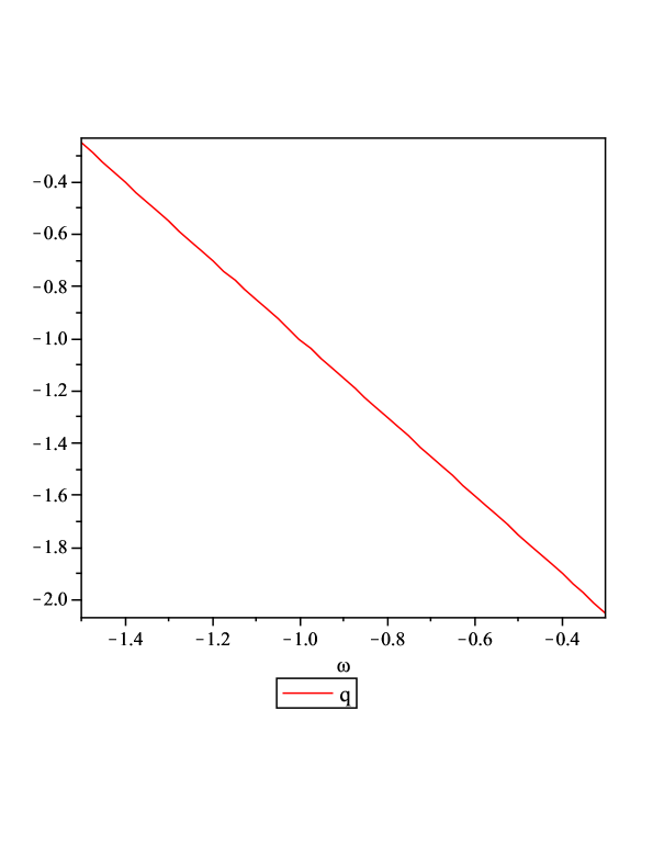
Figure 6: The deceleration parameter $q$ is plotted against $x$.

For $-1.6<\omega_{X}<0$, we notice that $q<0$, thus giving accelerated expansion of the universe (see Fig. 6). We further check the stability of the dynamical system (Eqs. 16 and 17) about the critical point ($u_{c},v_{c}$). To do this, we linearize the governing equations about the critical point i.e. $u=u_{c}+\delta u$ and $v=v_{c}+\delta v$, we obtain

$$\frac{d\delta u}{dx} = 3v_{c}\delta u+3(-1+u_{c})\delta v,$$ (23)

$$\frac{d\delta v}{dx} = \Big{[}\frac{-3\alpha}{u_{c}^{2}}(v^{2}_{c}+cv_{c})\Big{]}\delta u$$ (24)

$$+\Big{[}3(1+2v_{c}+\alpha)+\frac{6\alpha v_{c}}{u_{c}}+\frac{3\alpha c}{u_{c}}+3(1+\alpha)(1+\omega_{X})\Big{]}\delta v.$$

The eigenvalues corresponding to the linearized system are

$$\lambda = \frac{1}{2(-2+c-\omega_{X})}[-6c(2+\omega_{X})+3(2+\alpha)(2+\omega_{X})^{2}$$ (25)

$$-3\sqrt{\alpha(2+\omega_{X})^{2}(-4c^{2}+4c(2+\omega_{X})+\alpha(2+\omega_{X})^{2})}],$$

$$\mu = \frac{1}{2(-2+c-\omega_{X})}[-6c(2+\omega_{X})+3(2+\alpha)(2+\omega_{X})^{2}$$ (26)

$$+3\sqrt{\alpha(2+\omega_{X})^{2}(-4c^{2}+4c(2+\omega_{X})+\alpha(2+\omega_{X})^{2})}].$$

To obtain stable critical point, the real parts of the eigenvalues must be negative. We notice that for $\alpha\geq 0$, $0<c<2+\omega_{X}$ and $\omega_{X}<0$, the two eigenvalues $\lambda$ and $\mu$ will be negative, giving a stable attractor solution at ($u_{c},v_{c}$) in the late time evolution governed by the FRW equations. For instance, taking $c=0.3$, $\omega_{X}=-1.2$ and $\alpha=0.2$ (generalized phantom energy), we have $\lambda=-1.86$ and $\mu=-3.69$; whilst for $\alpha=1$ (phantom energy), we have $\lambda=-1.64$ and $\mu=-6.99$. The negativity of the eigenvalues can also be proven as

$$-6c(2+\omega_{X})+3(2+\alpha)(2+\omega_{X})^{2}=3(2+\omega_{X})(-2c+(2+\alpha)(2+\omega_{X}))\geq 0,$$ (27)

since $\alpha\geq 0$, $0<c<2+\omega_{X}$ and $\omega_{X}<0$. Now notice that both the eigenvalues will be negative if

$$(-6c(2+\omega_{X})+3(2+\alpha)(2+\omega_{X})^{2}\geq 9\alpha(2+\omega_{X})^{2}(-4c^{2}+4c(2+\omega_{X})+\alpha(2+\omega_{X})^{2}).$$ (28)

which yields

$$36(1+\alpha)(2+\omega_{X}-c)^{2}\geq 0.$$ (29)

Therefore both the eigenvalues are indeed negative. In Figures 1 and 2, we have provided a pictorial relationship between $u$ and $v$ for suitable choices of model parameters and initial conditions. It is interesting to notice that solutions converge to the same state under the given conditions. Figures 3 and 4 show that the functions $u$ and $v$ are stable solutions of the system i.e. the corresponding curves become flat at approximately $x\simeq 3$ and become globally flat afterwards. Initially these functions are unstable for small values of e-folding time $x$ but in the late times, these become globally stable. It can also be seen that NCG state parameter $\omega_{X}=v/u$ crosses $\omega_{X}=-1$ at present time ($x=0$) and enters the phantom regime $\omega_{X}<-1$ for large e-folding time (see Fig.5).

3 Conclusion

Model of interacting dark energy possesses enormous potential in resolving or at least simplifying several cosmological problems including the coincidence problem and the phantom crossing. In this model, these problems are analyzed by considering two major cosmic components namely dark matter and dark energy and assuming an interaction between them. Two non-conserving equations are derived and then non-dimensionalized. Due to non-linearity in the governing equations, we sought for numerical solution of the system. The stability of the solution is determined by performing stability analysis. In this paper, we have studied an interacting dark energy model dealing with the interaction between new generalized Chaplygin gas and the matter. The analysis is performed by doing the stability check of the dynamical system. We found that the dynamical system is stable about the only critical point of the system. This shows that stable stationary attractor solution exists in the late time evolution of the universe when the later one enters a steady state. Finally, this paper presents an extension of earlier work in [25].

Acknowledgment

I would like to thank anonymous referees for their useful criticism on this work.

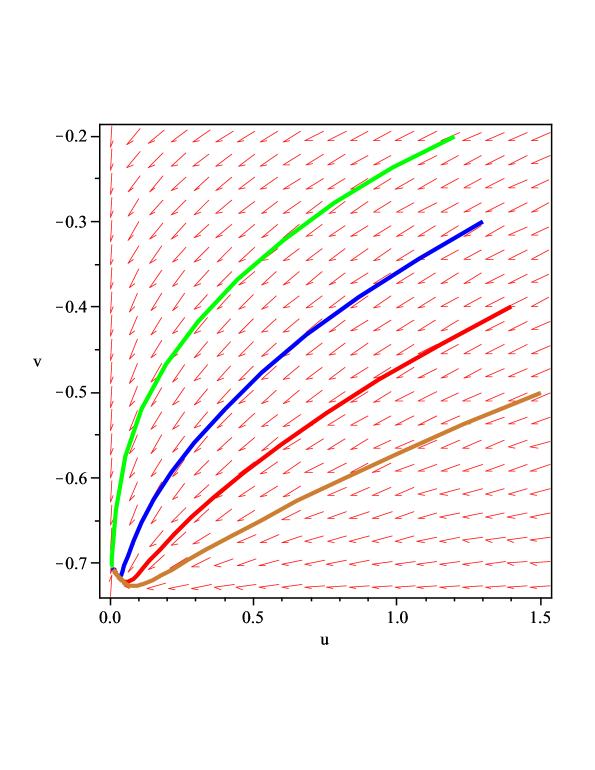
Figure 1: The phase diagram of the interacting new generalized Chaplygin gas model with $c=0.7$, $\alpha=0.07$ and $\omega_{X}=-1.3$. The curves correspond to the initial conditions $u(-2)=1.2,v(-2)=-0.2$ (green); $u(-2)=1.3,v(-2)=-0.3$ (blue); $u(-2)=1.4,v(-2)=-0.4$ (red); $u(-2)=1.5,v(-2)=-0.5$ (brown).

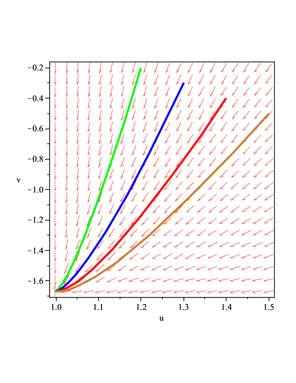
Figure 2: The phase diagram of the interacting new generalized Chaplygin gas model with $c=0.003$, $\alpha=0.3$, $\omega_{X}=-1/3$. The curves correspond to the initial conditions as given in Fig. 1.

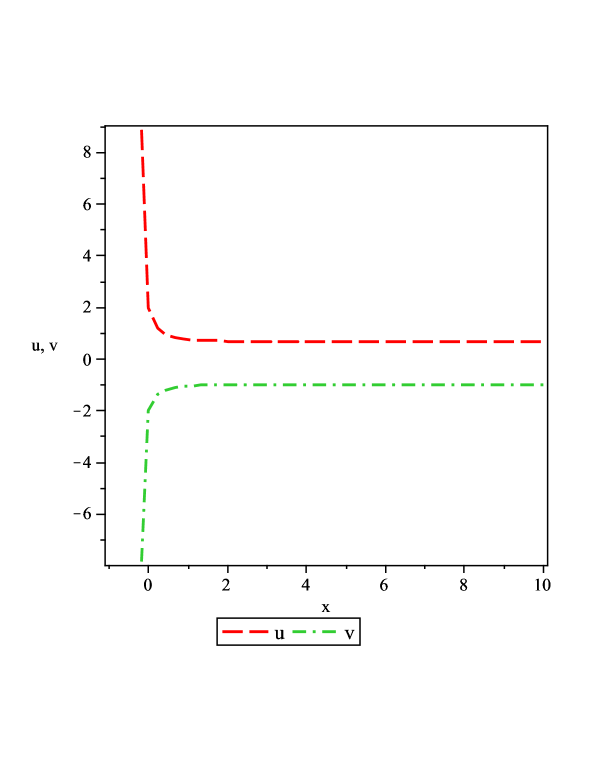
Figure 3: The parametric functions $u$ and $v$ are plotted against the e-folding time parameter $x$. The parameters are fixed as $c=0.3$, $\alpha=0.4$ and $\omega_{X}=-1$. The initial condition is $u(0)=2,v(0)=-2$.

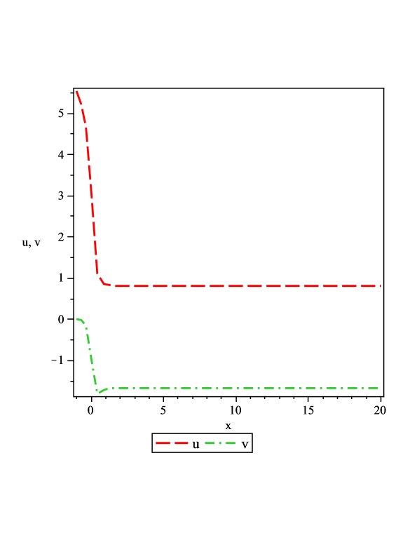
Figure 4: The parametric functions $u$ and $v$ are plotted against the e-folding time parameter $x$. The parameters are fixed as $c=0.5$, $\alpha=0.08$ and $\omega_{X}=-1/3$. The initial condition is $u(0)=3,v(0)=-1$.

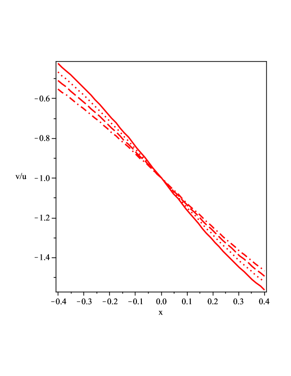
Figure 5: The EoS parameter $\omega_{X}=v/u$ is plotted against $x$. The parameters are fixed as $c=0.5$, $\alpha=0.08$ and $\omega_{X}=-1$. The initial conditions are $u(0)=1,v(0)=-1$ (solid line); $u(0)=1.1,v(0)=-1.1$ (dots); $u(0)=1.2,v(0)=-1.2$ (dashes); $u(0)=1.3,v(0)=-1.3$ (dash dot).

References

- [1] A.G. Riess et al, (Supernova Search Team Collaboration), Astron. J. 116 (1998) 1009; S. Perlmutter et al, (Supernova Cosmology Project Collaboration), Astrophys. J. 517 (1999) 565; C.L. Bennett et al, Astrophys. J. Suppl. Ser. 148 (2003) 175; M. Tegmark et al, (Sloan Digital Sky Survey Collaboration) Phys. Rev. D 69 (2004) 103501.
- [2] R.R. Caldwell and M. Kamionkowski, arXiv:0903.0866v1 [astro-ph.CO]; T. Padmanabhan, Phys. Rep. 380 (2003) 325; P.J.E. Peebles and B. Ratra, Rev. Mod. Phys. 75 (2003) 559; V. Sahni and A. Starobinsky, Int. J. Mod. Phys. D 15 (2006) 2105; M. Sami, Lect. Notes Phys. 72 (2007) 219; ibid, arXiv:0904.3445 [hep-th]; E.J. Copeland et al, Int. J. Mod. Phys. D 15 (2006) 1753; T. Buchert, Gen. Rel. Grav. 40 (2008) 467
- [3] N. Bachall et al, Science 284 (1999) 1481
- [4] S. Nojiri and S.D. Odintsov, AIP Conf. Proc. 1115 (2009) 212; ibid, Phys. Rev. D 77 (2008) 026007; ibid, Gen. Rel. Grav. 36 (2004) 1765; G. Cognola et al, Phys. Rev. D 73 (2006) 084007
- [5] L. Jarv et al, Phys. Rev. D 78 (2008) 083530; T. Tamaki, Phys. Rev. D 77 (2008) 124020; H. Motavali et al, Phys. Lett. B 666 (2008) 10
- [6] C. Garraffo et al, J. Math. Phys. 49 (2008) 042502; S.H. Mazharimousavi and M. Halilsoy, Phys. Lett. B 665 (2008) 125
- [7] K. Freese and M. Lewis, Phys. Lett. B 540 (2002) 1; S. Sen and A.A. Sen, Astrophys. J. 588 (2003) 1; Z.H. Zhu and M.K. Fujimoto, Astrophys. J. 602 (2004) 12
- [8] I. Brevik and O. Gorbunova, Gen. Rel. Grav. 37 (2005) 2039; G.M. Kremer and F.P. Devecchi, Phys. Rev. D 67 (2003) 047301; I. Brevik, Grav. Cosmol. 14 (2008) 332
- [9] K.A. Malik and D. Wands, Cosmological Perturbations, Physics Reports (2009), doi 10.1016/j.physrep.2009.03.001
- [10] A.Y. Kamenshchik et al, Phys. Lett. B 511 (2001) 265
- [11] N. Bilic et al, Phys. Lett. B 535 (2002) 17; M.C. Bento et al, Phys. Rev. D 66 (2002) 043507; M.C. Bento et al, Phys. Rev. D 73 (2006) 043504
- [12] H. Zhang and Z.H. Zhu, arXiv:0704.3121 [astro-ph]
- [13] O. Bertolami et al, arXiv:astro-ph/0402387v2; A.A. Sen, R.J. Scherrer Phys. Rev. D 72 (2005) 063511; R. Colistete Jr. and J.C. Fabris, Class. Quant. Grav. 22 (2005) 2813
- [14] L.D. Jun and L.X. Zhon, Chin. Phys. Lett. 22 (2005) 1600; T. Giannantonio and A. Melchiorri, Class. Quant. Grav. 23 (2006) 4125; J.C. Fabris et al, Gen. Rel. Grav. 36 (2004) 2559
- [15] M. Bordemann and J. Hoppe, Phys. Lett. B 317 (1993) 315; J.C. Fabris et al, Gen. Rel. Grav. 34 (2002) 53
- [16] M.C. Bento et al, Phys. Lett. B 75 (2003) 172
- [17] J.A.S. Lima et al, Class. Quantum Grav. 25 (2008) 205006; S. Li et al, arXiv:0809.0617 [gr-qc]; X. Chen and Y. Gong, arXiv:0811.1698 [gr-qc]; M.R. Setare, arXiv:hep-th/0609104; ibid, Eur. Phys. J. C 52 (2007) 689; H.M. Sadjadi and M. Alimohammadi, Phys. Rev. D 74 (2006) 103007; L.P. Chimento and A.S. Jakubi, Phys. Rev. D 67 (2003) 087302; Z.K. Guo et al, arXiv:astro-ph/0702015v3; N. Cruz et al, Phys. Lett. B 663 (2008) 338; T. Koivisto and D.F. Mota, arXiv:0707.0279 [astro-ph]; T. Clifton an J.D. Barrow, Phys. Rev. D 73 (2006) 104022; G.M. Phys. Rev. D 68 (2003) 123507; Y.B. Wu et al, Gen. Rel. Grav. 39 (2007) 653; M.R. Setare, Phys. Lett. B 648 (2007) 329; ibid, Int. J. Mod. Phys. D 18 (2009) 419; ibid, Eur. Phys. J. C 52 (2007) 689
- [18] N.P. Neto and B.M.O. Fraga et al, Gen. Rel. Grav. 40 (2008) 1653; M. Quartin et al, arXiv:0802.0546 [astro-ph]; L.P. Chimento et al, arXiv:astro-ph/0407288; W. Zimdahl and D. Pavon, Class. Quantum Grav. 24 (2007) 5461; N. Dalal et al, Phys. Rev. Lett. 87 (2001) 141302; H.M. Sadjadi, arXiv:0902.2462 [gr-qc]; ibid, arXiv:0904.1349 [gr-qc]; M.R. Setare, Phys. Lett. B 654 (2007) 1; J. Lee et al, Phys. Lett. B 661 (2008) 67; J.D. Barrow and T. Clifton, Phys. Rev. D 73 (2006) 103520; I. Zlatev et al, Phys. Rev. Lett. 82 (1999) 896; W. Zimdahl and D. Pavon, Gen. Rel. Grav. 36 (2004) 1483; M. Jamil and M.A. Rashid, Eur. Phys. J. C 60 (2009) 141; S. Chattopadhyay and U. Debnath, arXiv:0901.2184 [gr-qc]; S. Das and N. Banerjee, Gen. Relativ. Gravit. 38 (2006) 785
- [19] M. Szydlowski, Phys. Lett. B 632 (2006) 1
- [20] B. Wang et al, Nuc. Phys. B 778 (2007) 69
- [21] O. Bertolami et al, Phys. Lett. B 654 (2007) 165
- [22] A. de la Macorra, Phys. Rev. D 76 (2007) 027301
- [23] S.M. Carroll et al, Phys. Rev. D 68 (2003) 023509
- [24] H. Zhang and Z-H Zhu, Phys. Rev. D 73 (2006) 043518
- [25] P. Wu and H. Yu, Class. Quantum Grav. 24 (2007) 4661
- [26] X. Zhang et al, JCAP 0601 (2006) 003; S. Chattopadhyay, U. Debnath, Grav. Cosmol. 14 (2008) 341
- [27] M.R. Setare and E.C. Vagenas, Phys. Lett. B 666 (2008) 111
- [28] C. Feng et al, Phys. Lett. B 665 (2008) 111