Diversity Analysis of Peaky FSK Signaling in Fading Channels

Abstract

Error performance of noncoherent detection of on-off frequency shift keying (OOFSK) modulation over fading channels is analyzed when the receiver is equipped with multiple antennas. The analysis is conducted for two cases: 1) the case in which the receiver has the channel distribution knowledge only; and 2) the case in which the receiver perfectly knows the fading magnitudes. For both cases, the maximum a posteriori probability (MAP) detection rule is derived and analytical probability of error expressions are obtained. Numerical and simulation results indicate that for sufficiently low duty cycle values, lower error probabilities with respect to FSK signaling are achieved. Equivalently, when compared to FSK modulation, OOFSK with low duty cycle requires less energy to achieve the same probability of error, which renders this modulation a more energy efficient transmission technique. Also, through numerical results, the impact of number of antennas, antenna correlation, duty cycle values, and unknown channel fading on the performance are investigated.

Index Terms: Diversity, duty factor, fading channels, frequency-shift keying, MAP detection, multiple antennas, on-off keying, probability of error.

I Introduction

Frequency-shift keying (FSK) is a modulation format that is well-known and well-studied in the communications literature [15]. FSK is an attractive transmission scheme due to its high energy efficiency and suitability for noncoherent communications. For instance, under unknown channel conditions, energy detection can be employed to detect the FSK signals. Indeed, the analysis of FSK modulation dates back to 1960s (see e.g., [1] and [2]). Recently, it has been shown in [5] that unless the channel conditions are perfectly known at the receiver, signals that have very high peak-to-average power ratio is required to achieve the capacity in the low-SNR regime. This has initiated work on peaky signaling. Luo and Médard [6] have shown that FSK with small duty cycle can achieve rates of the order of capacity in ultrawideband systems with limits on bandwidth and peak power. In [8], the authors have studied the error performance of peaky FSK signaling over multipath fading channels by obtaining upper and lower bounds on the error probability. In [9], on-off frequency-shift keying (OOFSK) is defined as FSK overlaid on on-off keying, and its capacity and energy efficiency is analyzed. Note that OOFSK can be seen as joint pulse position modulation (PPM) and FSK. In this signaling, peakedness is introduced in both time and frequency. The error performance of OOFSK signaling when the transmitter and receiver are each equipped with a single antenna is recently studied in [10].

One of the important techniques to improve the performance in wireless communications is to use multiple antennas to achieve diversity gain. Considerable amount of work has been done on multiple reception channels [19]. In [2], it is shown for binary and $M$-ary signaling over Rician fading channels that increasing the number of reception channels can improve the error performance significantly. By finding the probability distribution function of the instantaneous SNR in flat fading multi-reception channels and substituting it into the probability of error expressions of PAM, PSK and QAM over an AWGN channel, the authors in [12] obtained expressions for the average probability of error of multi-reception fading channels. In [14], the probability of error of BPSK over Rician fading multi-reception channels is given and extensions to other modulation techniques are discussed. In [18], average symbol error rate of selection diversity of $M$-ary FSK modulated signal transmitted over fading channels is studied.

In this paper, the error performance of noncoherent detection of OOFSK over multiple reception Rician fading channels is studied. In Section II, the system model is presented. In Section III, the error performance in unknown Rician fading channels is studied. In Section IV, we investigate the error performance in known fading channels. Finally, Section V includes our conclusions.

II System Model

OOFSK modulation is employed at the transmitter. In OOFSK modulation, the transmitted signal during the symbol interval $0\leq t\leq T_{s}$ can be expressed as

$$s_{m}(t)=\left\{\begin{array}[]{ll}\sqrt{\frac{P}{v}}e^{j(w_{m}t+\theta_{m})}&m=1,2,3,\ldots M\\ 0&m=0\end{array}\right.$$ (3)

where $w_{m}$ and $\theta_{m}$ are the frequency in radians per second and phase, respectively, of the signal $s_{m}(t)$ when $m\neq 0$. Note that we have $M$ FSK signals and a zero signal denoted by $s_{0}(t)$. The frequencies of the FSK signals are chosen so that the signals are orthogonal. Since noncoherent detection of OOFSK signals is considered throughout the paper, the phases $\theta_{m}$ can be arbitrary. It is assumed that an FSK signal $s_{m}(t)$, $m\neq 0$, is transmitted with a probability of $\frac{v}{M}$ while $s_{0}(t)$ is transmitted with a probability of $1-v$ where $v$ is the duty cycle of the transmission. With these definitions, it is easily seen that $P$ and $\frac{P}{v}$ are the average and peak powers, respectively, of the modulation technique. Therefore, constraints on the peak power will impose lower bounds on the values that the duty cycle parameter $v$ can assume.

The receiver is equipped with $L$ antennas that enable the multiple reception of the transmitted signal. If, without loss of generality, we assume that $s_{k}(t)$ is the transmitted signal, the received signal at the $l^{\text{th}}$ antenna is

$$r_{l}(t)=h_{l}s_{k}(t)+n_{l}(t)\quad l=1,2,\ldots,L$$ (4)

where $h_{l}$ is the fading coefficient of the $l^{\text{th}}$ reception channel and $n_{l}(t)$ is a white Gaussian noise process with single-sided spectral density of $N_{0}$. It is assumed that the additive Gaussian noise components at different antennas are independent. Furthermore, the received signal model (4) presumes that the fading is frequency-flat and slow enough so that the fading coefficients stay constant over one symbol duration.

Following each antenna, there is a bank of $M$ correlators, each correlating the received signal with one of the orthogonal frequencies. The output of the $m^{\text{th}}$ correlator employed after the $l^{\text{th}}$ antenna is given by

$$Y_{l,m} =\frac{1}{\sqrt{N_{0}T_{s}}}\int_{0}^{T_{s}}r_{l}(t)e^{-jw_{m}t}dt$$ (5)

$$=\left\{\begin{array}[]{ll}Ah_{l}e^{j\theta_{m}}+n_{l,m}&m=k\\ n_{l,m}&m\neq k\end{array}\right.$$ (8)

where $n_{l,m}$ is a circularly symmetric complex Gaussian random variable with zero-mean and a variance of $1$ (due to normalization with $\frac{1}{\sqrt{N_{0}T_{s}}}$) and for notational convenience, we have defined $A=\sqrt{\frac{PT_{s}}{vN_{0}}}$. Since the frequencies are orthogonal and the additive Gaussian noise is independent at each antenna, $\{n_{l,m}\}$ for $l\in\{1,\ldots,L\}$ and $m\in\{1,\ldots,M\}$ forms an independent and identically distributed (i.i.d.) sequence. Note also that $R_{l,m}=|Y_{l,m}|^{2}$ gives the energy present in the $m^{\text{th}}$ frequency at the $l^{th}$ antenna.

III Noncoherent Detection of OOFSK with Channel Distribution Knowledge Only

III-A Detection Rule

In this section, we assume that the realizations of the fading coefficients $\{h_{l}\}$ are unknown at both the receiver and transmitter. The receiver is only equipped with the knowledge of the statistics of $\{h_{l}\}$. We further assume that $\{h_{l}\}$ are i.i.d. complex Gaussian random variables with $E\{h_{l}\}=d_{l}$ and $Var\{h_{l}\}=\sigma^{2}$. Hence, we consider a Rician fading channel model which specializes to Rayleigh fading when $d_{l}=0$. With the described channel statistics, conditioned on $s_{k}(t)$ being the transmitted signal, $Y_{l,m}$ is a complex Gaussian random variable with

$$\begin{split}E\{Y_{l,m}|s_{k}\}&=\left\{\begin{array}[]{ll}Ad_{l}e^{j\theta_{k}}&m=k\\ 0&m\neq k\end{array}\right.,\text{ and}\\ Var\{Y_{l,m}|s_{k}\}&=\left\{\begin{array}[]{ll}A^{2}\sigma^{2}+1&m=k\\ 1&m\neq k\end{array}\right..\end{split}$$ (9)

The receiver is assumed to perform noncoherent energy detection and therefore compute $R_{l,m}=|Y_{l,m}|^{2}$ after the correlator. $R_{l,m}$ is chi-square distributed with the following conditional probability density function (pdf) given the transmitted signal $s_{k}$ [15]:

$$f_{R_{l,m}|\,s_{k}}(R_{l,m})=\left\{\begin{array}[]{ll}\!\!\!\!\frac{1}{\sigma_{y}^{2}}\,e^{-\frac{R_{m}+A^{2}|d_{l}|^{2}}{\sigma_{y}^{2}}}I_{0}\left(\frac{2A|d_{l}|\sqrt{R_{m}}}{\sigma_{y}^{2}}\right)&\!m=k\\ \!\!\!\!e^{-R_{l,m}}&\!m\neq k\end{array}\right.$$ (12)

where $\sigma_{y}^{2}=A^{2}\sigma^{2}+1$ and $I_{0}(\cdot)$ is the zeroth order modified Bessel function of the first kind. It is assumed that the receiver, using equal gain combining, combines the energies of the $m^{\text{th}}$ frequency component at each antenna, i.e., computes the total energy

$$R_{m}=\sum_{l=1}^{L}R_{l,m}.$$

Since the additive noise components and fading coefficients at different antennas are independent, $R_{m}$ is a sum of independent chi-square random variables, and is itself also chi-square distributed with $2L$ degrees of freedom. Hence, the conditional pdf of $R_{m}$ is given by [15]

$$f_{R_{m}|s_{k}}(R_{m})\!=\!\left\{\begin{array}[]{ll}\!\!\!\!\frac{1}{\sigma_{y}^{2}}\left(\frac{R_{m}}{\xi}\right)^{\frac{L-1}{2}}e^{-\frac{R_{m}+\xi}{\sigma_{y}^{2}}}I_{L-1}\left(\frac{2\sqrt{R_{m}\xi}}{\sigma_{y}^{2}}\right)&\!\!m=k\\ \!\!\!\!\frac{R_{m}^{L-1}}{\Gamma(L)}\,e^{-R_{m}}&\!\!m\neq k\end{array}\right.$$ (15)

where $\xi=A^{2}\sum_{l=1}^{L}|d_{l}|^{2}$, $I_{L-1}(\cdot)$ is the $(L-1)^{\text{th}}$ order modified Bessel function of the first kind, and $\Gamma(\cdot)$ is the gamma function.

The receiver employs maximum a posteriori probability (MAP) criterion to detect the transmitted signals. Let ${\mathbf{R}}=[R_{1},R_{2},\ldots,R_{M}]$ be the vector of energy values corresponding to each frequency. Since the noise components $n_{l,m}$ are independent for different $m\in\{1,\ldots,M\}$, the components of ${\mathbf{R}}$ are mutually independent. Hence, the conditional pdf of ${\mathbf{R}}$ is given by the product of the marginal pdf’s (see equation (18) on the next page).

$$f_{{\mathbf{R}}|s_{k}}({\mathbf{R}})=\left\{\begin{array}[]{ll}\frac{1}{\sigma_{y}^{2}}\left(\frac{R_{k}}{\xi}\right)^{\frac{L-1}{2}}e^{-\frac{R_{k}+\xi}{\sigma_{y}^{2}}}I_{L-1}\left(\frac{2\sqrt{R_{k}\xi}}{\sigma_{y}^{2}}\right)\prod_{\begin{subarray}{c}n=1\\ n\neq k\end{subarray}}^{M}\frac{R_{n}^{L-1}e^{-R_{n}}}{\Gamma(L)},&k\neq 0\\ \frac{1}{\left[\Gamma(L)\right]^{M}}\prod_{n=1}^{M}R_{n}^{L-1}e^{-R_{n}},&k=0\end{array}\right..$$ (18)

 

Note that given the decision variables ${\mathbf{R}}=[R_{1},R_{2},\ldots,R_{M}]$, MAP detection minimizes the error probabilities [15]. The MAP decision rule that detects $s_{k}$ for $k\neq 0$ is

$$f_{{\mathbf{R}}|s_{k}}>f_{{\mathbf{R}}|s_{m}}\quad\forall m\neq 0,k\quad\text{and}\quad f_{{\mathbf{R}}|s_{k}}>\frac{M(1-v)}{v}f_{{\mathbf{R}}|s_{0}}$$ (19)

where we have used the fact that the prior probabilities of the transmitted signals are $p(s_{m})=\frac{v}{M}$ for all $m\neq 0$, and $p(s_{0})=(1-v)$. Substituting (18) into (19), we can simplify the decision rule to

$$\begin{split}g_{1}(R_{k})&>g_{1}(R_{m})\quad\forall m\neq k\quad\text{and}\\ g_{1}(R_{k})&>\frac{M(1-v)\sigma_{y}^{2}e^{\frac{\xi}{\sigma_{y}^{2}}}\xi^{\frac{L-1}{2}}}{v(L-1)!}\end{split}$$ (20)

where $g_{1}(R_{k})=R_{k}^{-\frac{L-1}{2}}e^{\frac{R_{k}A^{2}\sigma^{2}}{\sigma_{y}^{2}}}I_{L-1}\left(\frac{2\sqrt{R_{k}\xi}}{\sigma_{y}^{2}}\right)$ with $\xi>0$.
The following Lemma enables us to further simplify the detection rule.

Lemma 1

The function

$$g_{1}(x)=x^{-\frac{L-1}{2}}e^{\frac{xA^{2}\sigma^{2}}{\sigma_{y}^{2}}}I_{L-1}\left(\frac{2\sqrt{x\xi}}{\sigma_{y}^{2}}\right)$$

for $x>0$ and $\xi>0$ is a monotonically increasing function of $x$. Moreover,

$$\lim_{x\to 0}g_{1}(x)=\frac{\xi^{\frac{L-1}{2}}}{\sigma_{y}^{2(L-1)}(L-1)!}.$$

Proof: The derivative of the $n{{}^{\text{th}}}$ order modified Bessel function is $\frac{dI_{n}(x)}{dx}=I_{n+1}(x)+\frac{n}{x}I_{n}(x)$ [17, Section 8.48]. Hence,

$$\frac{dI_{L-1}(\frac{2\sqrt{x\xi}}{\sigma_{y}^{2}})}{dx} =\frac{1}{\sigma_{y}^{2}}\sqrt{\frac{\xi}{x}}I_{L}\left(\frac{2\sqrt{x\xi}}{\sigma_{y}^{2}}\right)+\frac{L-1}{2x}I_{L-1}\left(\frac{2\sqrt{x\xi}}{\sigma_{y}^{2}}\right)$$ (21)

$$>\frac{L-1}{2x}I_{L-1}\left(\frac{2\sqrt{x\xi}}{\sigma_{y}^{2}}\right)$$ (22)

where we have used the fact that $\sqrt{\frac{\xi}{x}}I_{L}\left(\frac{2\sqrt{x\xi}}{\sigma_{y}^{2}}\right)>0$ for $x>0$. Then, the derivative of $g_{1}(\cdot)$ satisfies (23) through (25) (see next page)

$$\frac{dg_{1}(x)}{dx} =-\frac{L-1}{2}x^{-\frac{L+1}{2}}e^{\frac{xA^{2}\sigma^{2}}{\sigma_{y}^{2}}}I_{L-1}\left(\frac{2\sqrt{x\xi}}{\sigma_{y}^{2}}\right)+x^{-\frac{L-1}{2}}e^{\frac{xA^{2}\sigma^{2}}{\sigma_{y}^{2}}}\frac{dI_{L-1}\left(\frac{2\sqrt{x\xi}}{\sigma_{y}^{2}}\right)}{dx}+\frac{A^{2}\sigma^{2}}{\sigma_{y}^{2}}x^{-\frac{L-1}{2}}e^{\frac{xA^{2}\sigma^{2}}{\sigma_{y}^{2}}}I_{L-1}\left(\frac{2\sqrt{x\xi}}{\sigma_{y}^{2}}\right)$$ (23)

$$>-\frac{L-1}{2}x^{-\frac{L+1}{2}}e^{\frac{xA^{2}\sigma^{2}}{\sigma_{y}^{2}}}I_{L-1}\left(\frac{2\sqrt{x\xi}}{\sigma_{y}^{2}}\right)+x^{-\frac{L-1}{2}}e^{\frac{xA^{2}\sigma^{2}}{\sigma_{y}^{2}}}\frac{L-1}{2x}I_{L-1}\left(\frac{2\sqrt{x\xi}}{\sigma_{y}^{2}}\right)+\frac{A^{2}\sigma^{2}}{\sigma_{y}^{2}}x^{-\frac{L-1}{2}}e^{\frac{xA^{2}\sigma^{2}}{\sigma_{y}^{2}}}I_{L-1}\left(\frac{2\sqrt{x\xi}}{\sigma_{y}^{2}}\right)$$ (24)

$$=\frac{A^{2}\sigma^{2}}{\sigma_{y}^{2}}x^{-\frac{L-1}{2}}e^{\frac{xA^{2}\sigma^{2}}{\sigma_{y}^{2}}}I_{L-1}\left(\frac{2\sqrt{x\xi}}{\sigma_{y}^{2}}\right)>0\quad\text{for }x>0$$ (25)

 

proving that $g_{1}(x)$ is a monotonically increasing function of $x>0$. Note that (24) follows from the lower bound expression provided in (22). Finally, the limit expression can be easily shown by using the series expansion $I_{L-1}\left(\frac{2\sqrt{x\xi}}{\sigma_{y}^{2}}\right)=x^{\frac{L-1}{2}}\left(\frac{\xi}{\sigma_{y}^{4}}\right)^{\frac{L-1}{2}}\sum_{k=0}^{\infty}\frac{\left(\frac{\xi x}{\sigma_{y}^{4}}\right)^{k}}{k!\Gamma(L+k)}$ [17, Section 8.44]. $\blacksquare$

With the result of Lemma 1, the decision rule in (19) now simplifies to

$$\begin{split}R_{k}&>R_{m}\quad\forall m\neq k\quad\text{and}\\ R_{k}&>\tau_{1}=\left\{\begin{array}[]{ll}g_{1}^{-1}(T_{1})&\text{if }T_{1}\geq\frac{\xi^{\frac{L-1}{2}}}{\sigma_{y}^{2(L-1)}(L-1)!}\\ 0&\text{otherwise}\end{array}\right.\end{split}$$ (26)

where $T_{1}=\frac{M(1-v)\sigma_{y}^{2}\xi^{\frac{L-1}{2}}e^{\frac{\xi}{\sigma_{y}^{2}}}}{v(L-1)!}.$ Since $g_{1}(\cdot)$ is a monotonically increasing function, $g_{1}^{-1}(T_{1})$ is well-defined for $T_{1}\geq\frac{\xi^{\frac{L-1}{2}}}{\sigma_{y}^{2(L-1)}(L-1)!}$. Finally, note that $s_{0}$ is the detected signal if $R_{k}<\tau_{1}$ for all $k$.

III-B Probability of Error

In this section, we analyze the error probability of OOFSK modulation when MAP detection is used at the receiver. Suppose without loss of generality that $s_{1}(t)$ is the transmitted signal. Then the correct detection probability is

$$P_{c,1} =P(R_{1}>R_{2},R_{1}>R_{3},\ldots,R_{1}>R_{M},R_{1}>\tau_{1}|s_{1})$$

$$=\int_{\tau{{}_{1}}}^{\infty}\left(\int_{0}^{x}f_{R_{2}|s_{1}}(t)\,dt\right)^{M-1}f_{R_{1}|s_{1}}(x)\,dx$$

$$=\int_{\tau{{}_{1}}}^{\infty}\left(\int_{0}^{x}\frac{t^{L-1}}{\Gamma(L)}e^{-t}dt\right)^{M-1}f_{R_{1}|s_{1}}(x)\,dx.$$

From [15], we know that $\int_{0}^{x}\frac{1}{\Gamma(L)}t^{L-1}e^{-t}dt=1-e^{-x}\sum_{l=0}^{L-1}\frac{x^{l}}{l!}$. Therefore, the correct detection probability can now be expressed as

$$P_{c,1} =\int_{\tau_{1}}^{\infty}\left[1-e^{-x}\sum_{l=0}^{L-1}\frac{x^{l}}{l!}\right]^{M-1}f_{R_{1}|s_{1}}(x)dx$$ (27)

$$=\int_{\tau_{1}}^{\infty}\sum_{n=0}^{M\!-\!1}(-1)^{n}\left(\!\!\!\begin{array}[]{cc}M\!-\!1\\ n\end{array}\!\!\!\right)\!\!\left[\sum_{l=0}^{L-1}\!\!\frac{x^{l}}{l!}e^{-x}\right]^{n}\!\!\!f_{R_{1}|s_{1}}(x)dx$$ (30)

where the rightmost expression is obtained using the binomial theorem. Moreover, multinomial expansion provides $\left[\sum_{l=0}^{L-1}\frac{x^{l}}{l!}e^{-x}\right]^{n}=e^{-nx}\sum_{i=0}^{n(L-1)}c_{in}x^{i}$ where $c_{in}$ is the coefficient of $x^{i}$ in the expansion. $c_{in}$ can be evaluated from the recursive equation $c_{in}=\sum_{q=i-L+1}^{i}\frac{c_{q(n-1)}}{(i-q)!}1_{[0,(n-1)(L-1)]}(q)\text{ where }1_{[a,b]}(q)=1\text{ for }a\leq q\leq b,\text{ and is equal to }0\text{ otherwise }\cite[cite]{[\@@bibref{}{marvin}{}{}]}.$ Using the multinomial expansion, $P_{c,1}$ can be expressed as in (40) on the next page.

$$P_{c,1} =\sum_{n=0}^{M-1}(-1)^{n}\left(\!\!\!\begin{array}[]{cc}M-1\\ n\end{array}\!\!\!\right)\sum_{i=0}^{n(L-1)}\!\!c_{in}\int_{\tau_{1}}^{\infty}\!\!x^{i}e^{-nx}f_{R_{1}|s_{1}}(x)dx$$ (33)

$$=\sum_{n=0}^{M-1}(-1)^{n}\left(\begin{array}[]{cc}M-1\\ n\end{array}\right)\sum_{i=0}^{n(L-1)}c_{in}\int_{\tau_{1}}^{\infty}x^{i}e^{-nx}\frac{1}{\sigma_{y}^{2}}\left(\frac{x}{\xi}\right)^{\frac{L-1}{2}}e^{-\frac{x+\xi}{\sigma_{y}^{2}}}I_{L-1}\left(\frac{2\sqrt{x\xi}}{\sigma_{y}^{2}}\right)dx$$ (36)

$$=\sum_{n=0}^{M-1}(-1)^{n}\left(\begin{array}[]{cc}M-1\\ n\end{array}\right)\sum_{i=0}^{n(L-1)}c_{in}\frac{\xi^{-\frac{L-1}{2}}e^{-\frac{\xi}{\sigma_{y}^{2}}}}{\sigma_{y}^{2}}\left[\frac{\xi^{\frac{L-1}{2}}(i+L)!}{2(1+n\sigma_{y}^{2})^{\frac{i+L}{2}}\sigma_{y}^{L-2-i}L!}F\left(-i,L,\frac{\xi}{\sigma_{y}^{2}(1+n\sigma_{y}^{2})}\right)\right.$$ (39)

$$\hskip 156.49014pt\left.\times e^{\frac{\xi}{\sigma_{y}^{2}(1+n\sigma_{y}^{2})}}-\int_{0}^{\tau_{1}}x^{\frac{2i+L-1}{2}}e^{-\frac{1+n\sigma_{y}^{2}}{\sigma_{y}^{2}}x}I_{L-1}\left(\frac{2\sqrt{x\xi}}{\sigma_{y}^{2}}\right)dx\right].$$ (40)

 

(40) is obtained by noting the following integration result from [2, Equation (81)]:

$$\int_{0}^{\infty} e^{-a^{2}x^{2}}x^{\mu-1}I_{\nu}(bx)dx$$

$$=\frac{b^{\nu}\Gamma\left(\frac{\mu+\nu}{2}\right)}{2^{\nu+1}a^{\mu+\nu}\Gamma(\nu+1)}e^{\frac{b^{2}}{4a^{2}}}F\left(\frac{\nu-\mu}{2}+1,\nu+1;\frac{-b^{2}}{4a^{2}}\right)$$

where $F(a,c;z)$ is the confluent hypergeometric function [16]. Note that while the correct detection probability $P_{c,1}$ can be numerically computed using (30), simplifications in numerical integration can be provided by (40) in which the integral has finite limits.

If $s_{0}(t)$ is the transmitted signal, the probability of correct detection is

$$P_{c,0} =P\left(R_{1}<\tau_{1},\ldots,R_{M}<\tau_{1}|s_{0}\right)=\left(1-e^{-\tau_{1}}\sum_{l=0}^{L-1}\frac{\tau_{1}^{l}}{l!}\right)^{M}.$$ (41)

Finally, the average probability of error is

$$P_{e}=1-(vP_{c,1}+(1-v)P_{c,0}).$$

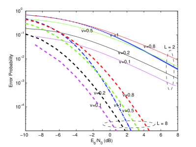
Figure 1: Error probability vs. $E_{b}/N_{0}$ (dB) for 8-OOFSK signaling over independent Rician fading channels with equal Rician factor $K=1$. The receiver has only channel distribution knowledge. Solid lines provide the error rates for $L=2$ channels while dashed lines are for $L=8$ channels. Duty cycle values are 0.1, 0.2, 0.5, 0.8, 1.

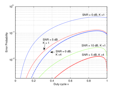
Figure 2: Error probability vs. duty cycle $v$ for 8-OOFSK signaling over $L=2$ independent Rician fading channels with equal Rician factor. The curves for which Rician factor is $K=1$ is plotted as solid lines while the curves for which $K=4$ are plotted as dotted-solid lines. The receiver has only channel distribution knowledge.

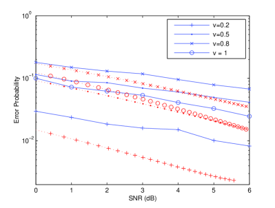
Figure 3: Error probability vs. SNR for 4-OOFSK signaling over two Rician fading channels (i.e., $L=2$) with equal Rician factor $K=\frac{1}{8}$. The receiver has only channel distribution knowledge. Curves with solid lines provide the error rates when the channels are correlated (correlation coefficient $\rho=\frac{1}{4}$) while dotted lines are for independent channels. Duty cycle values are 0.2, 0.5, 0.8, 1.

Next, we present the numerical results. We define the Rician factor as $K=\frac{|E\{h_{l}\}|}{E\{|h_{l}-E\{h_{l}\}|^{2}\}}=\frac{|d_{l}|^{2}}{\sigma^{2}}$ and correlation coefficient as $\rho=\frac{\text{cov}(h_{i},h_{j})}{\sqrt{\text{var}(h_{i})\text{var}(h_{j})}}$. Figure 1 plots the computed error probability curves for different duty cycle, $v$, values when 8-OOFSK signals are transmitted over unknown independent Rician fading channels all with the same Rician factor of $K=1$. Solid lines provide the error rates for $L=2$ channels while dashed lines are for $L=8$ channels. Note that in $M$-OOFSK modulation, the maximum number of bits that can be carried on the average is equal to the entropy $H(v)=v\log_{2}(M/v)+(1-v)\log_{2}(1/(1-v))$ bits/symbol which decreases to zero as $v\to 0$. Hence, decreasing the duty cycle diminishes the data rates. Therefore, for fair comparison, Fig. 1 plots the curves as a function of the SNR normalized by the entropy of the $M$-OOFSK signaling, giving the SNR per bit or equivalently $E_{b}/N_{0}$. In this figure, we observe that for sufficiently small $E_{b}/N_{0}$ values, the highest error rates are seen when $\nu=1$ (i.e., when conventional FSK is employed). In fact, we can show that as $\text{SNR}\to 0$, the error probabilities approach $P_{e}\to v$ when $v<M/(M+1)$, and $P_{e}\to(M-v)/M$ when $v>M/(M+1)$ (see Appendix A). Hence, asymptotically as SNR vanishes, error probabilities when $v<(M-1)/M$ are smaller than those attained when $v=1$. Note that when $M=8$, $(M-1)/M=0.875$, confirming the above-mentioned observation in Fig. 1. However, we also see in this figure that as $E_{b}/N_{0}$ increases, conventional FSK (i.e., OOFSK with $v=1$) achieves lower error rates than those achieved when $v=0.8$ and $v=0.5$. For instance, when $L=2$, conventional FSK out performs OOFSK with $v=0.8$ and $v=0.5$ when $E_{b}/N_{0}$ is greater than $-4.6$ dB and $4.4$ dB, respectively. Similar behavior is observed for the case of $L=8$ when $E_{b}/N_{0}$ exceeds $-6.6$ dB and $-1.3$ dB. Note that the impact of the minimum distance in the constellation on error rates is pronounced when SNR increases. Note further that for OOFSK modulation with $v<1$, the minimum distance between the transmitted signals is proportional to $\sqrt{P/v}$ while the minimum distance for conventional orthogonal FSK is proportional to $\sqrt{2P}$. Hence, in contrast to the low-SNR regime, gains at moderate SNR levels are expected only if $v<0.5$, as evidenced in the graphs of $v=0.2$ and $\nu=0.1$ where the duty factor is sufficiently decreased, and hence consequently the minimum distance is increased. Note that when $\nu=0.1$, we observe approximately an order of magnitude improvement with respect to FSK modulation. Fig. 1 also demonstrates the diversity benefits of increasing the number of reception channel from $L=2$ to $L=8$. As SNR grows without bound, we can show that $P_{e}\to 0$ for all values of $v\in(0,1]$, and hence any possible gains in the error performance obtained by increasing the peakedness diminishes.

Fig. 2 plots the error probabilities as a function of the duty cycle parameter $v$ for 8-OOFSK signaling over two independent Rician channels with identical Rician factor values. Fig. 2 confirms the earlier observation that improvements in error rates at moderate-to-high SNR levels are realized if $v$ is sufficiently small. We observe that the values of $v$ required to produce improvements are in general dependent on SNR and the Rician factor $K$, and get smaller with increasing SNR and $K$. For instance, when SNR = 0 dB and $K=1$, error rates lower than those achieved by FSK signaling is attained when $v<0.77$. On the other hand, when SNR = 5 dB and $K=4$, $v$ should be lowered below 0.53. Finally, Fig. 3 provides a comparison between the performances in correlated and independent channels. The error rates for correlated channels with correlation coefficient $\rho=1/4$ are obtained through simulations (rather than computations) by using the decision rules derived for independent channels. In this figure, we immediately note the deterioration in the performance due to channel correlation.

IV Noncoherent Detection of OOFSK with Instantaneous Channel Knowledge

IV-A Detection Rule

In this section, we assume that the instantaneous values of $|h_{l}|$ for all $l$ are perfectly known to the receiver while the phases of the fading coefficients, $\theta_{h}$, are still unknown. We further assume that the transmitter has no knowledge of the fading coefficients. Similarly as in the previous section, the receiver first computes the energy of each frequency at each antenna through $R_{m,l}=|Y_{m,l}|^{2}$. Conditioned on $|h_{l}|$ and the transmitted signal $s_{k}$, the pdf of the chi-squared distributed $R_{l,m}$ is given by [15]

$$f_{R_{l,m}|\,|h_{l}|,s_{k}}(R_{l,m})=$$

$$\quad\left\{\begin{array}[]{ll}e^{-(R_{l,m}+A^{2}|h_{l}|^{2})}I_{0}\left(2A|h_{l}|\sqrt{R_{l,m}}\right)&m=k\\ e^{-R_{l,m}}&m\neq k\end{array}\right..$$ (44)

When we compare the statistics of the $R_{l,m}$ in Sections III and IV (i.e., compare (12) and (44)), we note that (44) can be obtained from (12) by assuming $\sigma^{2}=0$ and replacing $|d_{l}|$ by the random channel magnitude $|h_{l}|$ in (12). Due to this similarity in the statistics, it can be seen that the results for the known channel can be obtained as a special case of those in Section III if we set $\sigma^{2}=0$ and replace $|d_{l}|$ by $|h_{l}|$ in the formulas in Section III. For instance, we again assume here that the receiver combines, for each frequency, the energies across the antennas, and obtain

$$R_{m}=\sum_{l=1}^{L}R_{l,m}=\sum_{l=1}^{L}|Y_{l,m}|^{2}.$$

It can be shown that the conditional pdf of the vector of sum energies, ${\mathbf{R}}=[R_{1},\ldots,R_{M}]$, is given by (47) on the next page

$$f_{{\mathbf{R}}||\mathbf{h}|,s_{k}}({\mathbf{R}})=\left\{\begin{array}[]{ll}\left(\frac{R_{k}}{\xi}\right)^{\frac{L-1}{2}}e^{-(R_{k}+\xi)}I_{L-1}(2\sqrt{R_{k}\xi})\prod_{n=1\ n\neq k}^{M}\frac{R_{n}^{L-1}e^{-R_{n}}}{\Gamma(L)}&k\neq 0\\ \frac{1}{\left[\Gamma(L)\right]^{M}}\prod_{n=1}^{M}R_{n}^{L-1}e^{-R_{n}}&k=0\end{array}\right.$$ (47)

 

where $\xi=A^{2}\sum_{l=1}^{L}|h_{l}|^{2}$, and $|\mathbf{h}|=[|h_{1}|,\ldots,|h_{L}|]$ is the vector of the magnitudes of the fading coefficients. Note that assuming $\sigma^{2}=0$ and replacing $|d_{l}|$ by $|h_{l}|$ in (18) also leads to (47). Using this approach, one can easily verify that the MAP rule that detects $s_{k}$ for $k\neq 0$ in known channels is

$$\begin{split}R_{k}&>R_{m}\,\,\forall m\neq k\qquad\text{and}\\ R_{k}&>\tau_{2}=\left\{\begin{array}[]{ll}g_{2}^{-1}(T_{2})&\text{if }T_{2}\geq\frac{\xi^{\frac{L-1}{2}}}{(L-1)!}\\ 0&\text{otherwise}\end{array}\right.\end{split}$$ (48)

where $g_{2}(R_{k})=R_{k}^{-\frac{L-1}{2}}I_{L-1}(2\sqrt{R_{k}\xi})$ and $T_{2}=\frac{M(1-v)e^{\xi}\xi^{\frac{L-1}{2}}}{v(L-1)!}$. Note that (48) is the rule that detects the signal $s_{k}(t)$ for $k\neq 0$. The zero signal $s_{0}(t)$ is detected if $R_{k}<\tau$ $\forall k.$

IV-B Probability of Error

We first assume that $s_{1}(t)$ is the transmitted signal. Then, specializing the results in Section III-B, we find the correct detection probability as

$$P_{c,1} =P(R_{1}>R_{2},R_{1}>R_{3},\ldots,R_{1}>R_{M},R_{1}>\tau_{2}|s_{1},|\mathbf{h}|)$$

$$=\int_{\tau_{2}}^{\infty}\left[1-e^{-x}\sum_{l=0}^{L-1}\frac{x^{l}}{l!}\right]^{M-1}f_{R_{1}||\mathbf{h}|,s_{1}}(x)dx$$ (49)

$$=\sum_{n=0}^{M-1}(-1)^{n}\left(\!\!\!\begin{array}[]{cc}M-1\\ n\end{array}\!\!\!\right)$$ (52)

$$\quad\sum_{i=0}^{n(L-1)}c_{in}\int_{\tau_{2}}^{\infty}x^{i}\left(\frac{x}{\xi}\right)^{\frac{L-1}{2}}e^{-[(n+1)x+\xi]}I_{L-1}(2\sqrt{x\xi})dx.$$ (53)

Note that if we specialize (40), an expression involving a hypergeometric function can also be obtained. The probability of correct detection when signal $s_{0}(t)$ is transmitted is

$$P_{c,0} =P\left(R_{1}<\tau_{2},\ldots,R_{M}<\tau_{2}||\mathbf{h}|,s_{0}\right)$$ (54)

$$=\left(1-e^{-\tau_{2}}\sum_{l=0}^{L-1}\frac{\tau_{2}^{l}}{l!}\right)^{M}.$$ (55)

Hence, the probability of error as a function of the instantaneous signal-to-noise ratio is

$$P_{e}=1-(vP_{c,1}+(1-v)P_{c,0}).$$ (56)

Since the channel is assumed to be known, error probability in (56) is a function of the fading coefficients through $\chi=\sum_{l=1}^{L}|h_{l}|^{2}$. Hence, the average probability of error is obtained by computing $\bar{P}_{e}=\int_{0}^{\infty}P_{e}\,f_{\chi}(\chi)d\chi.$ If $h_{l}$ is a complex Gaussian random variable with mean value $d_{l}$ and variance $\sigma^{2}$ and $\{h_{l}\}$ are mutually independent, $\chi$ is a chi-square random variable with $2L$ degrees of freedom and has a pdf given by $f_{\chi}(\chi)=\frac{1}{\sigma^{2}}\left(\frac{\chi}{s^{2}}\right)^{\frac{L-1}{2}}e^{-\frac{\chi+s^{2}}{\sigma^{2}}}I_{L-1}\left(\frac{2\sqrt{\chi s^{2}}}{\sigma^{2}}\right)$ where, $s^{2}=\sum_{l=1}^{L}|d_{l}|^{2}$.

When the fading coefficients $\{h_{l}\}$ are correlated, the average error probability $\bar{P}_{e}$ can be obtained by evaluating the expected value of $P_{e}$ with respect to the joint distribution of $(|h_{1}|,\ldots,|h_{L}|)$, which involves an $L$-fold integration. However, if $\{|h_{l}|\}$ are Nakagami-$m$ distributed, closed-form expressions for $f_{\chi}(\chi)$ are provided in [20], which lead to a single integration.

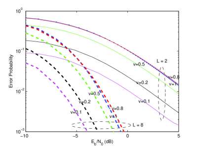
Figure 4: Error probability vs. $E_{b}/N_{0}$ (dB) for 8-OOFSK signaling over independent Rician fading channels with equal Rician factor $K=1$. The receiver has the knowledge of the instantaneous values of the fading magnitude. Solid lines provide the error rates for $L=2$ channels while dashed lines are for $L=8$ channels. Duty cycle values are 0.1, 0.2, 0.5, 0.8, 1.

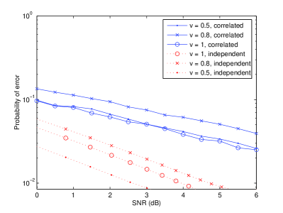
Figure 5: Error probability vs. SNR for 4-OOFSK signaling over two correlated known Rician fading channels with equal Rician factor $K=\frac{1}{8}$ and correlation coefficient $\rho=\frac{1}{4}$. Duty factor values are $v=1,0.8,0.5$, and $0.2$.

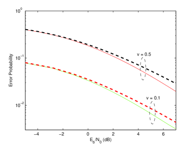
Figure 6: Error probability vs. $E_{b}/N_{0}$ (dB) for 8-OOFSK signaling over two independent Rayleigh fading channels, i.e., $L=2$. Solid curves provide the error rates when the fading magnitude is perfectly known at the receiver while dashed curves are the error rates when the receiver has only channel distribution knowledge.

Figure 4 plots, for different values of $v$ and different number of reception channels, the computed error probability vs. $E_{b}/N_{0}$ curves for 8-OOFSK over known independent Rician fading channels each with $K=1$. Conclusions similar to that in Section III can be immediately drawn here. However, note that error performance improves even when $v=0.5$ in this case. When $v=0.2$ and 0.1, even lower error probabilities are attained. Equivalently, we can conclude that for fixed error rates, substantial energy gains are realized, rendering OOFSK signaling a very energy efficient transmission technique. In Fig. 5, a comparison between the performances in correlated and independent channels is given. Although the performance is deteriorated due to correlation, OOFSK with sufficiently small duty factor still considerably improves the error performance. Finally, in Fig. 6, we plot the error probabilities for 8-OOFSK signaling with $v=0.5$ and $v=0.1$ over both known and unknown Rayleigh fading channels. We note that knowing the fading magnitudes does not provide benefits at low $E_{b}/N_{0}$ values. At relatively high values of the bit energy, approximately 1 dB gain in $E_{b}/N_{0}$ can be achieved for fixed error rates. Note that in known and unknown channels, detection rules are similar and hence the implementation complexities of the detectors are comparable. However, in order to get the performance results of the known channels, channels have to be estimated at the receiver. Therefore, gains in the performance should be compared with the resources expended for channel estimation to identify the net gains.

V Conclusion

In this paper, we have analyzed the error performance of OOFSK modulation in both known and unknown fading channels when the receiver is equipped with multiple antennas. The receiver is assumed to obtain the sum energy for each frequency by combining the energies of that frequency present at each antenna. We have identified the MAP detection rules as comparisons of the sum energies of frequencies with each other and a certain threshold, and obtained analytical error probability expressions. Through numerical and simulation results, we have shown the benefits of increasing the peakedness of the signals, and quantified the impacts of the number of antennas, antenna correlation, duty cycle values, and unknown channel conditions on the error performance.

Appendix A

In obtaining the asymptotic values of the error probabilities, the critical step is to find the value of the threshold $\tau_{1}$ in (26) as SNR vanishes. When $v<\frac{M}{M+1}$, we can see from the definitions in (26) that

$$\lim_{\text{SNR}\to 0}\frac{g_{1}(\tau_{1})}{T_{1}}=1$$ (57)

from which we can easily deduce that $\tau_{1}\to\infty$ as SNR decreases. Then, from the correct detection probabilities in (30) and (41), we have $\lim_{\text{SNR}\to 0}P_{c,1}=0$ and $\lim_{\text{SNR}\to 0}P_{c,0}=1$, which lead to

$$\lim_{\text{SNR}\to 0}P_{e}=\lim_{\text{SNR}\to 0}(1-vP_{c,1}-(1-v)P_{c,0})=v.$$

On the other hand, when $v>\frac{M}{M+1}$, we can find again from (26) that $\tau_{1}\to 0$ as SNR $\to 0$. In this case, we readily obtain that $\lim_{\text{SNR}\to 0}P_{c,1}=\frac{1}{M}$ and $\lim_{\text{SNR}\to 0}P_{c,0}=0$, which lead to

$$\lim_{\text{SNR}\to 0}P_{e}=\lim_{\text{SNR}\to 0}(1-vP_{c,1}-(1-v)P_{c,0})=1-\frac{v}{M}=\frac{M-v}{M}.$$

References

• [1] J. R. Pierce, β€œUltimate performance of $M$-ary transmissions on fading channels,” IEEE Trans. Inform. Theory, vol.Β IT-12, pp.Β 2-5, Jan. 1966.
• [2] W. C. Lindsey, β€œError probabilities for Rician fading multichannel reception of binary and N-ary signals,” IEEE Trans. Inform. Theory, pp.Β 330-350, Oct. 1964.
• [3] J. C. Hancock and W. C. Lindsey, β€œOptimum performance of self-adaptive communication system operating through a Rayleigh-fading medium,” IEEE Trans. Commun. Systems., vol.Β CS-11, pp.Β 443-454, Dec. 1963.
• [4] C. W. Helstrom, Statistical Theory of Signal Detection, New York, Pergamon Press, 1968.
• [5] S. VerdΓΊ, β€œSpectral efficiency in the wideband regime,” IEEE Trans. Inform. Theory, vol.Β 48, pp.Β 1319-1343, June 2002.
• [6] C. Luo and M. MΓ©dard, β€œFrequency-shift keying for ultrawideband - Achieving rates of the order of capacity,” Proc. 40th Annual Allerton Conference on Communication, Control, and Computing, Monticello, IL, 2002.
• [7] D. S. Lun, M. MΓ©dard, and I. C. Abou-Faycal, β€œOn the performance of peaky capacity-achieving signaling on multipath fading channels,” IEEE Trans. Commun., vol.Β 52, pp.Β 931-938, June 2004.
• [8] D. S. Lun, M. MΓ©dard and I. C. Abou-Faycal, β€œOn performance of peaky capacity-achieving signaling on multipath fading channels,” IEEE Trans. Commun., vol.Β 52, no.Β 6, pp.Β 931-938, June 2004.
• [9] M. C. Gursoy, H. V. Poor and S. Verdu, β€œOn-Off frequency-shift keying for wideband fading channels,” EURASIP Journal on Wireless Communications and Networking, 2006.
• [10] Q. Wang and M. C. Gursoy, β€œError performance of OOFSK signaling over fading channels,” Conference on Information Sciences and Systems (CISS), Princeton University, Princeton, NJ, 2006.
• [11] N. L. Johnson and S. Kotz, Continuous univariate distributions, New York, Wiley, 1970.
• [12] H. Zhang and T. A. Gulliver, β€œError probability for maximum ratio combing multichannel reception for M-ary coherent system over flat Ricean fading channels,” IEEE Wireless Communications and Networking Conference, vol. 1, 21-25 Mar. 2004, pp.Β 306-310.
• [13] D. D. N. Bevan, V. T. Ermolayev and A. G. Flaksman, β€œCoherent multiple reception of binary modulated signals with dependent Rician fading channel,” IEE Proceedings-Communications, vol.Β 48, issue 2, pp.Β 105-111, Apr. 2001.
• [14] V. V. Veeravalli and A. Mantravadi, β€œPerformance analysis for diversity reception of digital signals over correlated fading channels,” IEEE Vehicular Technology Conference, vol. 2, 16-20 May 1999, pp.Β 1291-1295.
• [15] J. G.Proakis, Digital Communications, New York, McGraw-Hill, 1989.
• [16] L. C. Andrews, Special Functions of Mathematics for Engineers, Oxford University Press, 1998.
• [17] I. S. Gradshteyn and I. M. Ryzhik, Table of Integrals, Series, and Products, Academic Press, 2000.
• [18] Y. Chen and N. C. Beaulieu, β€œSER of selection diversity MFSK with channel estimation errors,” IEEE Trans. Wireless Commun., vol.Β 5, no.Β 7, pp.Β 1920-1928, July 2006.
• [19] M. K. Simon and M. S. Alouini, Digital Communication over Fading Channels, New York, John Wiley & Sons, 2000.
• [20] G. K. Karagiannindis, N. C. Sagias and T. A. Tsiftsis, β€œClosed-form statistics for the sum of squared Nakagami-m variates and its applications,” IEEE Trans. Commun., volΒ 54, no.Β 8, pp.Β 1353-1359, Aug. 2006.
• [21] P. Gupta, N. Bansal and R. K. Mallik, β€œAnalysis of minimum selection H-S/MRC in Rayleigh channel,” IEEE Trans. Commun., vol.Β 53, no.Β 5, pp.Β 780-784, May 2005.