Structure Formation by Fifth Force I: N-Body vs. Linear Simulations

Abstract

We lay out the frameworks to numerically study the structure formation in both linear and nonlinear regimes in general dark-matter-coupled scalar field models, and give an explicit example where the scalar field serves as a dynamical dark energy. Adopting parameters of the scalar field which yield a realistic CMB spectrum, we generate the initial conditions for our N-body simulations, which follow the spatial distributions of the dark matter and the scalar field by solving their equations of motion using the multilevel adaptive grid technique. We show that the spatial configuration of the scalar field tracks well the voids and clusters of dark matter. Indeed, the propagation of scalar degree of freedom effectively acts a fifth force on dark matter particles, whose range and magnitude are determined by the two model parameters $(\mu,\gamma)$, local dark matter density as well as the background value for the scalar field. The model behaves like the $\Lambda$CDM paradigm on scales relevant to the CMB spectrum, which are well beyond the probe of the local fifth force and thus not significantly affected by the matter-scalar coupling. On scales comparable or shorter than the range of the local fifth force, the fifth force is perfectly parallel to gravity and their strengths have a fixed ratio $2\gamma^{2}$ determined by the matter-scalar coupling, provided that the chameleon effect is weak; if on the other hand there is a strong chameleon effect (i.e., the scalar field almost resides at its effective potential minimum everywhere in the space), the fifth force indeed has suppressed effects in high density regions and shows no obvious correlation with gravity, which means that the dark-matter-scalar-field coupling is not simply equivalent to a rescaling of the gravitational constant or the mass of the dark matter particles. We show these spatial distributions and (lack of) correlations at typical redshifts ($z=0,1,5.5$) in our multi-grid million-particle simulations. The viable parameters for the scalar field can be inferred on intermediate or small scales at late times from, e.g., weak lensing and phase space properties, while the predicted Hubble expansion and linearly simulated CMB spectrum are virtually indistinguishable from the standard $\Lambda$CDM predictions.

I Introduction

The origin and nature of dark energy Copeland (2006) is one of the most difficult challenges facing physicists and cosmologists now. Among all the proposed models to tackle this problem, a scalar field is perhaps the most popular one up to now. The scalar field, denoted by $\varphi$, might only interact with other matter species through gravity, or have a coupling to normal matter and therefore producing a fifth force on matter particles. The latter idea has seen a lot of interests in recent years, in the light that such a coupling could alleviate the coincidence problem of dark energy and that it is commonly predicted by low energy effective theories from a fundamental theory.

Nevertheless, if there is a coupling between the scalar field and baryonic particles, then stringent experimental constraints might be placed on the fifth force on the latter provided that the scalar field mass is very light (which is needed for the dark energy). Such constraints severely limit the viable parameter space of the model. Different ways out of the problem have been proposed, of which the simplest one is to have the scalar field coupling to dark matter only but not to standard model particles, therefore evading those constraints entirely. This is certainly possible, especially because both dark matter and dark energy are unknown to us and they may well have a common origin. Another interesting possibility is to have the chameleon mechanism Khoury (2004, 2004); Mota (2006, 2006), by virtue of which the scalar field acquires a large mass in high density regions and thus the fifth force becomes undetectablly short-ranged, and so also evades the constraints.

Study of the cosmological effect of a chameleon scalar field shows that the fifth force is so short-ranged that it has negligible effect in the large scale structure formation Brax (2004) for certain choices of the scalar field potential. But it is possible that the scalar field has a large enough mass in the solar system to pass any constraints, and at the same time has a low enough mass (thus long range forces) on cosmological scales, producing interesting phenomenon in the structure formation. This is the case of some $f(R)$ gravity models Carroll (2004); Nojiri (2003), which survives solar system tests thanks again to the chameleon effect Navarro (2007); Li (2007); Hu (2007); Brax (2008). Note that the $f(R)$ gravity model is mathematically equivalent to a scalar field model with matter coupling.

No matter whether the scalar field couples with dark matter only or with all matter species, it is of general interests to study its effects in cosmology, especially in the large scale structure formation. Indeed, at the linear perturbation level there have been a lot of studies about the coupled scalar field and $f(R)$ gravity models which enable us to have a much clearer picture about their behaviors now. But linear perturbation studies do not conclude the whole story, because it is well known that the matter distribution at late times becomes nonlinear, making the behavior of the scalar field more complex and the linear analysis insufficient to produce accurate results to confront with observations. For the latter purpose the best way is to perform full N-body simulations Bertschinger (1998) to evolve the individual particles step by step.

N-body simulations for scalar field and relevant models have been performed before Linder (2003); Mainini (2003); Springel (2007); Kesden (2006); Farrar (2007); Keselman (2009); Maccio (2004); Baldi (2008). For example, in Maccio (2004) the simulation is about a specific coupled scalar field model. This study however does not obtain a full solution to the spatial configuration of the scalar field, but instead simplifies the simulation by assuming that the scalar field’s effect is to change the value of the gravitational constant, and presenting an justifying argument for such an approximation. As we will see below, this approximation is only good in certain parameter spaces and for certain choices of the scalar field potential, and therefore we believe fuller simulations than the one performed in Maccio (2004) is needed to study the scalar field behavior most rigorously. Note also the structure formation with a coupled chameleon scalar field has also been studied using non B-body techniques previously Brax (2006).

Recently there have also appeared full simulations of the $f(R)$ gravity model Oyaizu (2008, 2008), which do solve the scalar degree of freedom explicitly. However, embedded in the $f(R)$ framework there are some limitations in the generality of these works. As a first thing, $f(R)$ gravity model (no matter what the form $f$ is) only corresponds to the couple scalar field models for a specific value of coupling strength Amendola (2007). Second, in $f(R)$ models the correction to standard general relativity is through the modification to the Poission equation and thus to the gravitational potential as a whole Oyaizu (2008), while in the coupled scalar field models we could clearly separate the scalar fifth force from gravity and analyze the former directly. Also, in $f(R)$ models the coupling between matter and the scalar field is universal (the same to dark matter and baryons), while in the couple scalar field models it is straightforward to switch on/off the coupling to baryons and study the effects on baryonic and dark matter clusterings respectively. And finally, the general framework of N-body simulations in couple scalar field models could also handle the situation where the chameleon effect is absent and scalar field only couples to dark matter (which is of no interests for $f(R)$ people).

In this article we present the general formulae and algorithm of full N-body simulations in coupled scalar field models and consider as an explicit example the results for a chameleon scalar field. Unlike in Maccio (2004), here we shall calculate the spatial distribution of the scalar field directly without making simplifications such as a rescaled gravitational constant. Neither shall we use the concept of varying-mass dark matter particles as in Maccio (2004), but instead we treat the system as constant-mass dark matter particles under the action of a fifth force.

The article is organized as follows: in § II we review the general equations of motion for the coupled scalar field model and introduce our specific choices of the coupling function and scalar field potential. Next we analyze in § III the general linear perturbation equations in the $3+1$ formalism Ellis (1989); Challinor (1999) and integrate them into the numerical Boltzmann code CAMB Lewis (2000) to study the effects on the linear structure formation. Then in § IV we turn to our main focus, introducing the formulae and algorithm of the N-body simulation. We also study the chosen model explicitly, display the preliminary results and discuss on them. Finally we conclude in § V.

II The Coupled Scalar Field Model

In this section we briefly introduce the model considered here and present the equations that will be analyzed in the following sections. Let us start by looking at the general field equations for a scalar field coupled to dark matter.

The Lagrangian for our coupled scalar field model is

$$\mathcal{L} = \frac{1}{2}\left[\frac{R}{\kappa}-\nabla^{a}\varphi\nabla_{a}\varphi\right]+V(\varphi)-C(\varphi)\mathcal{L}_{\mathrm{CDM}}+\mathcal{L}_{\mathrm{S}}\ \$$ (1)

where $R$ is the Ricci scalar, $\kappa=8\pi G$ with $G$ Newton’s constant, $\varphi$ is the scalar field, $V(\varphi)$ is its potential energy and $C(\varphi)$ its coupling to dark matter, which is assumed to be cold and described by the Lagrangian $\mathcal{L}_{\mathrm{CDM}}$. $\mathcal{L}_{\mathrm{S}}$ includes all the terms for photons, neutrinos and baryons, and these will be considered only when we calculate the large scale structure formation in the next section.

The dark matter Lagrangian, for a point-like particle with (bare) mass $m_{0}$, is

$$\mathcal{L}_{\mathrm{CDM}}(\mathbf{y}) = -\frac{m_{0}}{\sqrt{-g}}\delta(\mathbf{y}-\mathbf{x}_{0})\sqrt{g_{ab}\dot{x}^{a}_{0}\dot{x}^{b}_{0}}$$ (2)

where $\mathbf{y}$ is the coordinate and $\mathbf{x}_{0}$ is the coordinate of the centre of the particle. From this equation it can be easily derived that

$$T^{ab}_{\mathrm{CDM}} = \frac{m_{0}}{\sqrt{-g}}\delta(\mathbf{y}-\mathbf{x}_{0})\dot{x}^{a}_{0}\dot{x}^{b}_{0}.$$ (3)

Also, because $g_{ab}\dot{x}^{a}_{0}\dot{x}^{b}_{0}=g_{ab}u^{a}u^{b}=1$ where $u^{a}$ is the four velocity of the dark matter particle, so the Lagrangian could be rewritten as

$$\mathcal{L}_{\mathrm{CDM}}(\mathbf{y}) = -\frac{m_{0}}{\sqrt{-g}}\delta(\mathbf{y}-\mathbf{x}_{0}),$$ (4)

which will be used below.

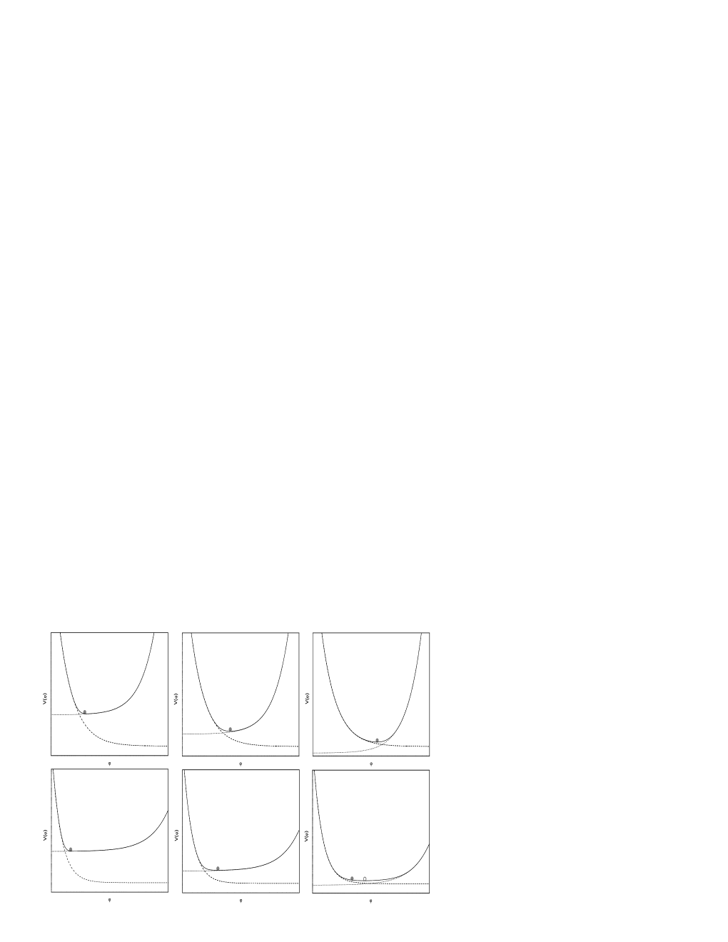
Figure 1: Upper panel: the potential (dashed curves), coupling function (dotted curves) and effective potential (solid curves) of the strong coupling scalar field model at various cosmic epochs. Lower panel: the same as the upper panel but for a coupling not strong enough so that the scalar field will not reside at the minimum of $V_{eff}$. Solid circles denote the states of the scalar field and in case that this does not coincide with the minimum of effective potential, the later is indicated by an open circle. See text for explanations.

Eq. (3) is the energy momentum tensor for a single dark matter particle. For a fluid with many particles the energy momentum tensor will be

$$T^{ab}_{\mathrm{CDM}} = \frac{1}{V}\int_{V}d^{4}y\sqrt{-g}\frac{m_{0}}{\sqrt{-g}}\delta(y-x_{0})\dot{x}^{a}_{0}\dot{x}^{b}_{0}$$ (5)

$$= \rho_{\mathrm{CDM}}u^{a}u^{b},$$

in which $V$ is a volume microscopically large and macroscopically small, and we have extend the 3-dimensional $\delta$ function to a 4-dimensional one by adding a time component.

Meanwhile, using

$$T^{ab} = -\frac{2}{\sqrt{-g}}\frac{\delta\left(\sqrt{-g}\mathcal{L}\right)}{\delta g_{ab}}$$ (6)

it is straightforward to show that the energy momentum tensor for the scalar field is given by

$$T^{\varphi ab} = \nabla^{a}\varphi\nabla^{b}\varphi-g^{ab}\left[\frac{1}{2}\nabla_{c}\varphi\nabla^{c}\varphi-V(\varphi)\right].$$ (7)

So the total energy momentum tensor is

$$T_{ab} = \nabla_{a}\varphi\nabla_{b}\varphi-g_{ab}\left[\frac{1}{2}\nabla_{c}\varphi\nabla^{c}\varphi-V(\varphi)\right]$$ (8)

$$+C(\varphi)T^{\mathrm{CDM}}_{ab}+T^{\mathrm{S}}_{ab}$$

where $T^{\mathrm{CDM}}_{ab}=\rho_{\mathrm{CDM}}u_{a}u_{b}$, $T^{\mathrm{S}}_{ab}$ is the energy momentum tensor for standard model particles, and the Einstein equation is

$$G_{ab} = \kappa T_{ab}$$ (9)

where $G_{ab}$ is the Einstein tensor. Note that due to the coupling between the scalar field $\varphi$ and the dark matter, the energy momentum tensors for either will not be conserved, and we have

$$\nabla_{b}T^{\mathrm{CDM}ab} = -\frac{C_{\varphi}(\varphi)}{C(\varphi)}\left(g^{ab}\mathcal{L}_{\mathrm{CDM}}+T^{\mathrm{CDM}ab}\right)\nabla_{b}\varphi\ \$$ (10)

where throughout this paper we shall use a _φ to denote the derivative with respect to $\varphi$.

Finally, the scalar field equation of motion (EOM) from the given Lagrangian is

$$\square\varphi+\frac{\partial V(\varphi)}{\partial\varphi} = \frac{\partial C(\varphi)}{\partial\varphi}\mathcal{L}_{\mathrm{CDM}}$$

where $\square=\nabla^{a}\nabla_{a}$. Using Eq. (4) it can be rewritten as

$$\square\varphi+\frac{\partial V(\varphi)}{\partial\varphi}+\rho_{\mathrm{CDM}}\frac{\partial C(\varphi)}{\partial\varphi} = 0.$$ (11)

Eqs. (8, 9, 10, 11) summarize all the physics that will be used in our analysis.

We will consider a special form for the scalar field potential,

$$V(\varphi) = \frac{V_{0}}{\left[1-\exp\left(-\sqrt{\kappa}\varphi\right)\right]^{\mu}},$$ (12)

where we have fixed the coefficient in front of $\varphi$ to be $1$ without loss of generality, since we can always rescale $\varphi$ to achieve this; $\mu$ is a dimensionless constant and $V_{0}$ is a constant with mass dimension $4$. As will be discussed below, we need $\mu\ll 1$ to evade local observational constraints. Meanwhile, the coupling between the scalar field and dark matter particle is chosen as

$$C(\varphi) = \exp(\gamma\sqrt{\kappa}\varphi),$$ (13)

where $\gamma>0$ is another dimensionless constant.

As will be explained below, the two dimensionless parameters $\mu$ and $\gamma$ have clear physical meanings: roughly speaking, $\mu$ controls the time when the effect of the scalar field becomes important in cosmology while $\gamma$ determines how important it would ultimately be. Indeed, the potential given in Eq. (12) is motivated by the $f(R)$ cosmology Li (2007), in which the extra degree of freedom behaves as a coupled scalar field in the Einstein frame. As we could see from Eq. (12), the potential $V\rightarrow\infty$ when $\varphi\rightarrow 0$ while $V\rightarrow V_{0}$ when $\varphi\rightarrow\infty$. In the latter case, however, $C\rightarrow\infty$, so that the effective total potential

$$V_{eff}(\varphi) = V(\varphi)+\rho_{\mathrm{CDM}}C(\varphi)$$ (14)

has a global minimum at some finite $\varphi$. If the total potential $V_{eff}(\varphi)$ is steep enough around this minimum, then the scalar field becomes very heavy and thus follows its minimum dynamically, as is in the case of the chameleon cosmology. If $V_{eff}$ is not steep enough at the minimum, however, the scalar field will have a more complicated evolution. These two different cases can be obtained by choosing appropriate values of $\gamma,\mu$: if $\gamma$ is very large or $\mu$ is small then we run into the former situation and if $\gamma$ is small and $\mu$ is large we have the latter.

In Fig. 1 we present a schematic plot of the two situations: the significant difference is that at late times when $\rho_{\mathrm{CDM}}$ becomes small, the effective potential becomes flat around its minimum if $\gamma$ is not very large and $\mu$ not very small, and as a result the true value of $\varphi$ will lag behind that corresponding to the minimum of $V_{eff}$. Of course if $V_{0}$ is chosen appropriately the scalar field can act as a dynamical dark energy in this slow-roll regime.

The complexity of the two cases also makes them phenomenologically rich, and it is of our interests to study how such a setup will affect the cosmology in background, linear perturbation and in particular nonlinear structure formation regimes. In the next two sections we shall consider these questions.

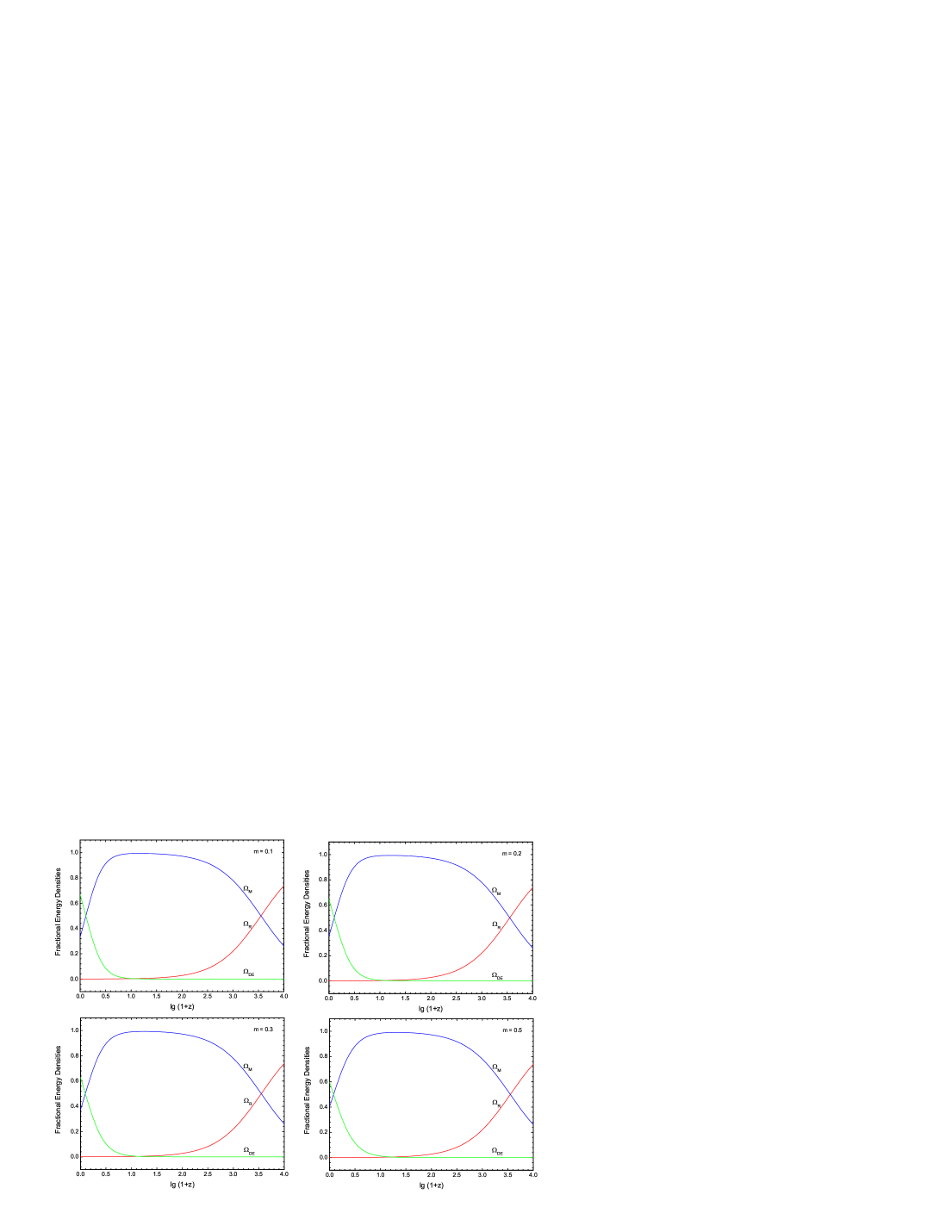
Figure 2: (Color Online) The evolution of the fractional energy densities in radiation (red lines), baryons + cold dark matter (blue lines) and scalar field dark energy component (green lines) with respect to $\lg(1+z)$ where $z$ is the redshift. The model parameters for this case are chosen by $\gamma=1$ and $\mu=0.1,0.2,0.3,0.5$ respectively. The physical parameters are $\Omega_{\mathrm{R}}=8.475\times 10^{-5}$ for radiation, $\Omega_{\mathrm{B}}=0.05$ for baryons, $\Omega_{\mathrm{\mathrm{CDM}}}=0.25$ for CDM and $H_{0}=70~{}\mathrm{km/s/Mpc}$ for the present Hubble expansion rate. To ensure these parameters the value of $V_{0}$ must be fine-tuned, and here we have used a trial-and-error method to adjust the value of $\lambda=\kappa V_{0}/3H_{0}^{2}$ as $0.53285,0.44868,0.38968,0.30848$ respectively for $\mu=0.1,0.2,0.3,0.5$. Note that given $H_{0}$ the propagations of the fractional energy densities fix the background evolution.

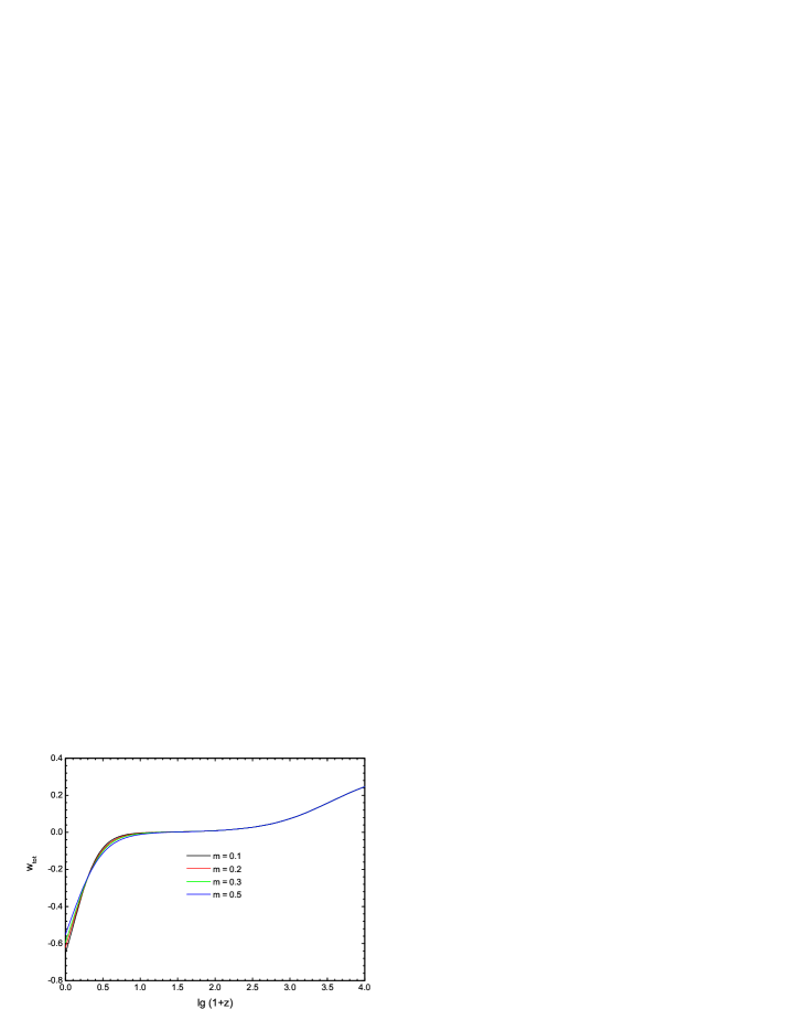
Figure 3: (Color Online) The total equation of state of the model with different values of $\mu$ as a function of $\lg(1+z)$. The parameters are the same as in Fig. 2 and the values of $\mu$ are given beneath the curves.

III Linear Structure Formation

Our first task is to linearize the model. Since this involves many equations, we refer the interested readers to the Appendices A and B for the complete first-order perturbation equations and their representations in $k$-space. We shall proceed then to study their effects on the large scale structure at linear perturbation level in the Universe by putting these linearize equations into the numerical Boltzmann code.

III.1 The Background Evolution

In what follows we will consider the limit of small $\mu$, $\mu\lesssim\mathcal{O}(0.1)$. It is then useful to define the effective mass of the scalar field by the Taylor expansion

$$V(\varphi) \approx V(\varphi_{0})+{m_{eff}^{2}\over 2}(\varphi-\varphi_{0})^{2}$$ (15)

where $\varphi_{0}$ is at the minimum of $V_{eff}$, given by

$${dV_{eff}(\varphi_{0})\ \over\ d\varphi}\ =\ 0 \rightarrow \sqrt{\kappa}\varphi_{0}\ \approx\ \frac{\mu}{\gamma}\frac{V_{0}}{\rho_{\mathrm{CDM}}},$$ (16)

in which we have used the facts that $1+\mu\approx 1$ as well as $\sqrt{\kappa}\varphi\ll 1$ so that $\exp(-\sqrt{\kappa}\varphi)\approx\exp(\gamma\sqrt{\kappa}\varphi)\approx 1$ and $1-\exp(-\sqrt{\kappa}\varphi)\approx\sqrt{\kappa}\varphi$. Thus the effective mass

$$m^{2}_{eff}$$

$$\equiv \frac{\partial^{2}V_{eff}(\varphi_{0})}{\partial\varphi^{2}_{0}},\quad y\equiv\exp(-\sqrt{\kappa}\varphi_{0})$$

$$= \mu\frac{\kappa V_{0}y}{\left[1-y\right]^{1+\mu}}\left[1+{(1+\mu)y\over 1-y}\right]+\gamma^{2}\kappa\rho_{\mathrm{C}DM}y^{-\gamma}$$

$$\approx \frac{(\gamma\kappa\rho_{\mathrm{C}DM})^{2}}{\kappa V_{0}}\left[{1+\mu\over\mu}+\ln{\mu V_{0}\over\gamma\rho_{\mathrm{C}DM}}+{(1+3\gamma)V_{0}\over\gamma\rho_{\mathrm{C}DM}}\right],$$

$$\approx \frac{(\gamma\kappa\rho_{\mathrm{C}DM})^{2}}{\mu\kappa V_{0}}$$ (18)

To see that the scalar field is heavy, i.e., $m^{2}_{eff}\gg H^{2}\sim H_{0}^{2}a^{-3}$, note that $\kappa\rho_{\mathrm{CDM}}\sim\mathcal{O}\left(H_{0}^{2}a^{-3}\right)\gg\mu\kappa V_{0}$, true for $\mu\ll 1$ [or $\mu\sim\mathcal{O}(1)$ but in the early universe, remember that we always assume $\gamma\sim\mathcal{O}(1)$]. This means that for $\mu\ll 1$ (or in the early times) the scalar field has a very heavy mass and tends to settle at $\varphi=\varphi_{0}$ (quickly oscillating there). Then as a good approximation we have

$$V(\varphi)\ \approx\ V(\varphi_{0})\ \approx\ V_{0}\left(\frac{\gamma\rho_{\mathrm{CDM}}}{V_{0}}\right)^{\mu}\left(\frac{1}{\mu}\right)^{\mu}\ \approx\ V_{0}\$$ (19)

in which we have used the facts that $\lim_{\mu\rightarrow 0^{+}}\mu^{\mu}=1$ in this regime. At the same time, because $\sqrt{\kappa}\dot{\varphi}\approx\sqrt{\kappa}\dot{\varphi_{0}}\approx-\frac{\mu}{\gamma}\frac{V_{0}}{\rho_{\mathrm{CDM}}}\frac{\dot{\rho}_{\mathrm{CDM}}}{\rho_{\mathrm{CDM}}}=3\sqrt{\kappa}\varphi_{0}H\ll H$ with the use of Eq. (16), so the kinetic energy of the scalar field is negligible. This shows that for small $\mu$ we do expect the scalar field to behave like a cosmological constant in background cosmology.

This analysis has been confirmed by numerical calculations. In Fig. 2 we show the fractional energy densities of the radiation, dust (baryon plus CDM) and dark energy (the scalar field) components for $\gamma=1$ and several values of $\mu$. It can be seen there the evolutions of these fractional energy densities are not sensitive to $\mu$. To see this more clearly we have also plotted in Fig. 3 the total equation of state of all matter species. As $\mu\rightarrow 0$ the curves quickly become indistinguishable from each other (and indistinguishable from the $\Lambda$CDM prediction).

III.2 The Linear Perturbation Evolution

To study the perturbation evolution and the effect of the scalar field on large scale structure formation, we just need to implement the perturbation equations listed in Appendix B into a Boltzmann code. As mentioned earlier, here we work in the $A=0$ frame, in which the CDM peculiar velocity $v_{\mathrm{CDM}}$ must be dynamically evolved according to Eq. (89) with $A=0$. Also note that the tight coupling approximation is not affected as compared with GR+$\Lambda$CDM.

The initial condition for $v_{\mathrm{CDM}}$ could be set to zero. In this way the observer is comoving with the dark matter particles initially (when the $\xi$ term in Eq. (81) is extremely small) and only deviate from the dark matter particle world lines when this $\xi$ term becomes significant. As for the initial conditions of $\xi$ and $\xi^{\prime}$, they are also very small at early times, and as we shall see below, there is good reason to set them to zero at those times. Thus we have adopted

$$\xi_{\mathrm{initial}} = 0,$$ (20)

$$\xi^{\prime}_{\mathrm{initial}} = 0,$$ (21)

$$v_{\mathrm{CDM,initial}} = 0,$$ (22)

as the initial conditions of the new variables which need to be evolved in the code.

In Fig. 4 we show a collect of the CMB power spectra for the model with $\gamma=0.5$. In Fig. 5 the matter power spectra of the corresponding parameter choices are given. We can see that the effect of the scalar field on the CMB spectrum is most significant for low-$\ell$ (large scales), and even there the effect is only to slightly reduce the power. This behavior is quite similar to the one found in Li (2007) and is due to the less decay of the gravitational potential on large scales at late times, which decreases the integrated Sachs-Wolfe (ISW) effect. Such small deviations of the CMB spectrum from the $\Lambda$CDM result are obviously not of much help in placing constraints on the model parameters $\mu$ and $\gamma$, especially because of the cosmic variance on large scales. Thus to distinguish this model from others we necessarily need to use other observables such as the linear (on large scales) and nonlinear (on smaller scales) matter power spectra.

To explain the matter power spectrum, let us consider the evolution of cold dark matter density contrast $\Delta_{\mathrm{CDM}}$ (A similar analysis is first given in Li (2007) for $f(R)$ model and later more generally in Tsujikawa (2007)). For simplicity we shall assume a Universe filled with only radiation and CDM particles. Taking the (conformal) time derivative of the equation

$$\Delta^{\prime}_{\mathrm{CDM}}+k\mathcal{Z}+kv_{\mathrm{CDM}} = 0,$$ (23)

we have

$$\Delta^{\prime\prime}_{\mathrm{CDM}}+k\mathcal{Z}^{\prime}+kv^{\prime}_{\mathrm{CDM}} = 0.$$ (24)

Taking the spatial derivative of Eq. (66), collecting the coefficients of harmonic expansions and using the frame choice $A=0$ we obtain

$$k\mathcal{Z}^{\prime}+k\frac{a^{\prime}}{a}\mathcal{Z}+\frac{\kappa}{2}(\mathcal{X}+3\mathcal{X}^{p})a^{2} = 0.$$ (25)

Substituting Eq. (25) into Eq. (24) and using Eqs. (89, 23) we arrive at

$$\Delta^{\prime\prime}_{\mathrm{CDM}}+\frac{a^{\prime}}{a}\Delta^{\prime}_{\mathrm{CDM}}-\frac{\kappa}{2}(\mathcal{X}+3\mathcal{X}^{p})a^{2}$$

$$+k\frac{C_{\varphi}}{C}(k\xi-\varphi^{\prime}v_{\mathrm{CDM}}) = 0,$$ (26)

where the last term is equal to $k\left(kA+v^{\prime}_{\mathrm{CDM}}+\frac{a^{\prime}}{a}v_{\mathrm{CDM}}\right)$ with $\xi$ being substituted using the propagation equation of $v_{\mathrm{CDM}}$ (remember that $A=0$ by choice of the frame).

Now according to Eq. (B.0.6) the evolution of $\xi$ is governed by

$$\xi^{\prime\prime}+2\frac{a^{\prime}}{a}\xi^{\prime}+(k^{2}+a^{2}V_{\varphi\varphi}+a^{2}\rho_{\mathrm{CDM}}C_{\varphi\varphi})\xi$$

$$+k\varphi^{\prime}\mathcal{Z}+a^{2}C_{\varphi}\rho_{\mathrm{CDM}}\Delta_{\mathrm{CDM}} = 0.\ \ \ \$$ (27)

For small scales (and late times) $k\gg|\frac{a^{\prime}}{a}|$ and the term $k^{2}\xi$ dominates over other terms proportional to $\xi$ in the above equations dominates so that the equation is approximately

$$k^{2}\xi+a^{2}C_{\varphi}\rho_{\mathrm{CDM}}\Delta_{\mathrm{CDM}} \doteq -k\varphi^{\prime}\mathcal{Z}$$ (28)

$$= \varphi^{\prime}\Delta^{\prime}_{\mathrm{CDM}}+k\varphi^{\prime}v_{\mathrm{CDM}}.$$ (29)

where we choose to eliminate $\mathcal{Z}$ by using Eq. (23). Substituting Eq. (29) into Eq. (III.2) to eliminate $\xi$ and $v_{\mathrm{CDM}}$, we get

$$\Delta^{\prime\prime}_{\mathrm{CDM}}+\left(\frac{a^{\prime}}{a}+\frac{C_{\varphi}}{C}\varphi^{\prime}\right)\Delta^{\prime}_{\mathrm{CDM}}$$

$$-\frac{\kappa}{2}(\mathcal{X}+3\mathcal{X}^{p})a^{2}-\frac{C^{2}_{\varphi}}{C}\rho_{\mathrm{CDM}}\Delta_{\mathrm{CDM}}a^{2} = 0.$$ (30)

During the matter dominated era we can neglect the contribution from radiation, and the above equation for the growth of the overdensity reduces to

$$\Delta^{\prime\prime}_{\mathrm{CDM}}+\tilde{H}\Delta^{\prime}_{\mathrm{CDM}} = 4\pi\tilde{G}\rho_{\mathrm{CDM}}\Delta_{\mathrm{CDM}}a^{2},$$ (31)

where

$$\tilde{G}\equiv\left(1+{2C_{\varphi}^{2}\over C}\right){\kappa\over 8\pi} \tilde{H}\equiv\frac{(aC)^{\prime}}{aC}.$$ , (32)

where $\kappa\equiv 8\pi G$ as before, and $2C_{\varphi}^{2}/C\approx 2\gamma^{2}$ for our coupling function of $C$ as given by Eq. (13). Thus we could see that the growth of cold dark matter density contrast is (on small scales) scale-independent, which explains the matter power spectrum at large $k$ values (small scales) in Fig. 5. In particular, note that for our choice of parameters we have $C\sim 1$ and $\tilde{H}=\frac{a^{\prime}}{a}+\frac{C^{\prime}}{C}\sim\frac{a^{\prime}}{a}$, and so this equation is approximately the same as that in the $\Lambda\mathrm{CDM}$ paradigm but with an effective gravitational constant $\tilde{G}\sim(1+2\gamma^{2})G$. This indicates that the parameter $\gamma$ characterizes the strength of the scalar field fifth force relative to gravity; the larger $\gamma$ is, the stronger the fifth force will ultimately be.

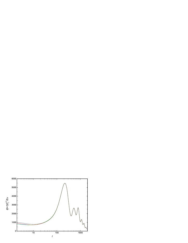
Figure 4: (Color Online) The CMB power spectra for the couple scalar field model with $\gamma=0.5$. The red, blue, green and black curves correspond to $\mu=0.1,0.2,0.3$ with chameleon perturbations and $\mu=0.1$ without chameleon perturbations, respectively. Curves for $\mu\lesssim 10^{-5}$ are indistinguishable from the $\Lambda$CDM result.

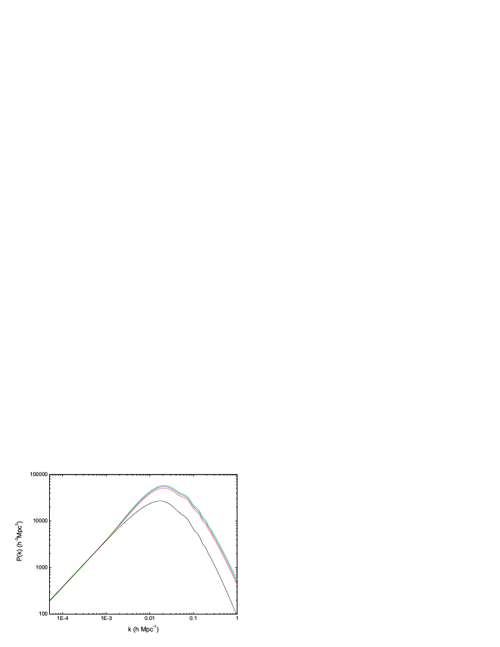
Figure 5: (Color Online) The matter power spectra for the couple scalar field model. The parameters are the same as in Fig. 4. The curves with $\mu\lesssim 10^{-5}$ are very close to the $\Lambda$CDM result.

Meanwhile, from the derivation process of Eq. (31) we see that the assumption that $k^{2}\gg a^{2}\left(V_{\varphi\varphi}+\rho_{\mathrm{CDM}}C_{\varphi\varphi}\right)$ [cf. Eq. III.2] has been used. This is of course true for our choices of $\mu$, but Eq. (III.1) tells us that this is not necessarily the case for $\mu\ll 1$, due to the strong nonlinearity of $V(\varphi)$. Let’s suppose now $k^{2}\ll a^{2}\left(V_{\varphi\varphi}+\rho_{\mathrm{CDM}}C_{\varphi\varphi}\right)$ for some small enough value of $\mu$ (say $\mu=10^{-7}$), then Eq. (III.2) should be approximated as

$$(a^{2}V_{\varphi\varphi}+a^{2}\rho_{\mathrm{CDM}}C_{\varphi\varphi})\xi+k\varphi^{\prime}\mathcal{Z}+a^{2}C_{\varphi}\rho_{\mathrm{CDM}}\Delta_{\mathrm{CDM}} \doteq 0$$

rather than as Eq. (28), so that in Eq. (III.2) the $k^{2}\xi$ term could be neglected, implying that the scalar field simply has negligible effects on the evolution of $\Delta_{\mathrm{CDM}}$. Thus we conclude that the effect of the parameter $\mu$ is to control the time when the fifth force becomes important as compared with gravity; the smaller $\mu$ is, the later will this time be. So with very strong chameleon effects (very nonlinear potentials) the fifth force could be greatly suppressed all through the cosmic history up to now, and it is therefore possible to get a cosmology very close to the $\Lambda$CDM paradigm in every aspect.

Obviously, at the very early times the fifth force is also suppressed even in cases of $\mu\sim\mathcal{O}(1)$, because in this regime again we have $k^{2}\ll a^{2}\left(V_{\varphi\varphi}+\rho_{\mathrm{CDM}}C_{\varphi\varphi}\right)$. Indeed this is the reason why we could set the initial condition as in Eq. (20).

Now the matter power spectra as seen in Fig. 5 could be well explained: when $\mu$ decreases, the time when the fifth force could fully show its power becomes later and as a result the growth of structure does not reach its maximum potential – this explains why the $\mu=0.1,0.2,0.3$ curves increasingly get far away from the black one. But because all these values of $\mu$ are large enough (compared with, say, $\mu=10^{-7}$), the fifth force in all these cases has almost realized its full power (which is $2\gamma^{2}$ times stronger than gravity according to Eq. (31)) – this explains why all the colored curves are fairly far from the black one. Finally, Eq. (31) explains why on small scales the colored $P(k)$ curves are almost parallel to the black one.

Given the complexity of the scalar field behavior, especially in regions with highly nonlinear matter distribution, we must say that the linear analysis performed above is only qualitatively correct and lacks the high precision to compare with various cosmological data sets. In particular, it may well be that the effect of the fifth force is not significant on linear scales because the fifth force is not long-range enough, but much more important on smaller scales which are beyond the linear regime. Thus in the next section we shall consider the scalar field model in the context of N-body cosmological simulations, and try to study its effects in a more accurate manner.

IV Nonlinear Structure Formation

In § III we have considered the background evolution and linear large structure formation in the couple scalar field model. For the former, the coupling between $\varphi$ and CDM prevents $\varphi$ from rolling to infinity and instead tends to keep $\varphi$ and $V(\varphi)$ constant; here we find that for a value of $\mu\lesssim\mathcal{O}(0.1)$ this effect is significant enough to make the background cosmology similar to that of $\Lambda$CDM. For the latter, the CMB spectrum is also not very sensitive to the value of $\mu$ or $\gamma$ such that $\mu\lesssim\mathcal{O}(0.1)$ is difficult to be distinguished from $\Lambda$CDM. These results suggest that large scale observables are not particularly well suited in studying the new features of this class of coupled scalar field models.

On smaller but still linear scales, we already see that the scalar field coupling effectively increases the gravitational force by a factor of $2\gamma^{2}$, leading to a significant increase in the small scale power of $P(k)$ for gravitational-strength couplings [$\gamma\sim\mathcal{O}(1)$]. One could of course argue that the observed matter power spectrum is indeed for the luminous matter only and cannot be applied to dark matter naïvely due to the bias between the two. But the enhancement of dark matter clustering in this model is abstract and can be tested by observations such as weak lensing without much ambiguity. If this is done, it is unlikely that there remains much space for such a strongly coupled model.

However, two things must be taken into account before we arrive at any definite conclusions about the fate of the model. First, on small scales where the scalar field effect becomes important, the distribution of matter is already beyond the linear perturbation regime and in some regions could be very nonlinear. This means that a linear analysis as presented in the above section is no longer sufficient and we must consider the nonlinear effect, which is most precisely taken in account by large N-body simulations. This will be the very topic of this section. Second, as we argued in § III, the behavior of the model is not only controlled by $\gamma$, but also by parameter $\mu$: for $\mu\ll 1$, the epoch when the scalar field fifth force starts to realizes its full power as $2\gamma^{2}$ times of gravity could be greatly postponed. It is then possible to prevent too powerful a structure formation.

Like in the background cosmology, this has something to do with nonlinear (chameleon) effects, but here things become much more complicated. In a homogeneous universe, the spatial gradient of the scalar field vanishes and the scalar field $\varphi$ takes the same value anywhere, largely simplifying the analysis. For the real universe with nonlinear matter distributions, the spatial gradient of $\varphi$ is normally much larger than the time derivative so that the configuration of the scalar field relies on the underlying matter distribution sensitively in a nonlinear way, and at the same time strongly affects the latter via the action of fifth force. Quantifying such complex couplings also calls for the use of N-body simulations.

In this paper we shall set up the basic framework of studying coupled scalar field models using N-body technique, putting much emphasis on the working mechanism and the fifth force effect. We shall start with a derivation of all the relevant equations of motion, describe how to integrate them into the numerical code and present some preliminary results. Detailed analysis will be postponed to companion papers. We will not provide an introduction to general N-body simulation techniques here, and interested readers are referred to the relevant literature Bertschinger (1998).

IV.1 The Nonrelativistic Equations

Our first step is to simplify the relevant equations of motion in the appropriate limit to get a set of equations which can be directly applied to the numerical code.

We know that the existence of the scalar field and its coupling to standard cold dark matter particles make the following changes to the $\Lambda$CDM model: First, the energy momentum tensor has a new piece of contribution from the scalar field; second, the energy density of dark matter is multiplied by a function $C(\varphi)$, which is because the coupling to scalar field essentially renormalizes the mass of dark matter particles; third and most important, dark matter particles will not follow geodesics in their motions as in $\Lambda$CDM, rather, the total force on them has a contribution from the scalar field.

These imply that the following things need to be modified or added:

1. The scalar field $\varphi$ equation of motion, which determines the value of the scalar field at any given time and position.

2. The Poisson equation, which determines the gravitational potential (and thus gravity) at any given time and position, according to the local energy density and pressure, which include the contribution from the scalar field (as obtained from $\varphi$ equation of motion) now.

3. The total force on the dark matter particles, which is determined by the spatial configuration of $\varphi$, just like gravity is determined by the spatial configuration of the gravitational potential.

We shall describe these one by one now.

For the scalar field equation of motion, we denote $\bar{\varphi}$ as the background value of $\varphi$ and $\delta\varphi\equiv\varphi-\bar{\varphi}$ as the scalar field perturbation. Then Eq. (11) could be rewritten as

$$\ddot{\delta\varphi}+3H\dot{\delta\varphi}+\vec{\nabla}_{\mathbf{r}}^{2}\varphi+V_{,\varphi}(\varphi)-V_{,\varphi}(\bar{\varphi})$$

$$+\rho_{\mathrm{CDM}}C_{,\varphi}(\varphi)-\bar{\rho}_{\mathrm{CDM}}C_{,\varphi}(\bar{\varphi}) = 0$$

by subtracting the corresponding background equation from it. Here $\vec{\nabla}_{\mathbf{r}a}$ is the covariant spatial derivative with respect to the physical coordinate $\mathbf{r}=a\mathbf{x}$ with $\mathbf{x}$ the conformal coordinate, and $\vec{\nabla}^{2}_{\mathbf{r}}=\vec{\nabla}_{\mathbf{r}a}\vec{\nabla}_{\mathbf{r}}^{a}$. $\vec{\nabla}_{\mathbf{r}a}$ is essentially the $\hat{\nabla}_{a}$, but because here we are working in the weak field limit we approximate it as $\vec{\nabla}_{\mathbf{r}}^{2}=-\left(\partial^{2}_{r_{x}}+\partial^{2}_{r_{y}}+\partial^{2}_{r_{z}}\right)$ by assuming a flat background; the minus sign is because our metric convention is $(+,-,-,-)$ instead of $(-,+,+,+)$. For the simulation here we will also work in the quasi-static limit, assuming that the spatial gradient is much larger than the time derivative, $|\vec{\nabla}_{\mathbf{r}}\varphi|\gg|\frac{\partial\varphi}{\partial t}|$ (which will be justified below). Thus the above equation can be further simplified as

$$c^{2}\partial_{\mathbf{x}}^{2}(a\delta\varphi)$$

$$= a^{3}\left[V_{,\varphi}(\varphi)-V_{,\varphi}(\bar{\varphi})+\rho_{\mathrm{CDM}}C_{,\varphi}(\varphi)-\bar{\rho}_{\mathrm{CDM}}C_{,\varphi}(\bar{\varphi})\right],$$

in which $\partial^{2}_{\mathbf{x}}=-\vec{\nabla}_{\mathbf{x}}^{2}=+\left(\partial^{2}_{x}+\partial^{2}_{y}+\partial^{2}_{z}\right)$ is with respect to the conformal coordinate $\mathbf{x}$ so that $\vec{\nabla}_{\mathbf{x}}=a\vec{\nabla}_{\mathbf{r}}$, and we have restored the factor $c^{2}$ in front of $\vec{\nabla}_{\mathbf{x}}^{2}$ (the $\varphi$ here and in the remaining of this paper is $c^{-2}$ times the $\varphi$ in the original Lagrangian unless otherwise stated). Note that here $V$ and $\rho_{\mathrm{CDM}}$ both have the dimension ofmass density rather than energy density.

Next look at the Poisson equation, which is obtained from the Einstein equation in weak-field and slow-motion limits. Here the metric could be written as

$$ds^{2} = (1+2\phi)dt^{2}-(1-2\psi)\delta_{ij}dr^{i}dr^{j}$$ (34)

from which we find that the time-time component of the Ricci curvature tensor $R^{0}_{\ 0}=-\vec{\nabla}_{\mathbf{r}}^{2}\phi$, and then the Einstein equation $R_{ab}=\kappa\left(T_{ab}-\frac{1}{2}g_{ab}T\right)$ gives

$$R^{0}_{\ 0}\ =\ -\vec{\nabla}_{\mathbf{r}}^{2}\phi\ =\ \frac{\kappa}{2}(\rho_{\mathrm{TOT}}+3p_{\mathrm{TOT}})$$ (35)

where $\rho_{\mathrm{TOT}}$ and $p_{\mathrm{TOT}}$ are respectively the total energy density and pressure. The quantity $\vec{\nabla}_{\mathbf{r}}^{2}\phi$ can be expressed in terms of the comoving coordinate $\mathbf{x}$ as

$$\vec{\nabla}_{\mathbf{r}}^{2}\phi = \frac{1}{a^{2}}\vec{\nabla}_{\mathbf{x}}^{2}\left(\frac{\Phi}{a}-\frac{1}{2}a\ddot{a}\mathbf{x}^{2}\right)$$ (36)

$$= \frac{1}{a^{3}}\vec{\nabla}_{\mathbf{x}}^{2}\Phi-3\frac{\ddot{a}}{a}$$

where we have defined a new Newtonian potential

$$\Phi \equiv a\phi+\frac{1}{2}a^{2}\ddot{a}\mathbf{x}^{2}$$ (37)

and used $\vec{\nabla}_{\mathbf{x}}^{2}\mathbf{x}^{2}=6$. Thus

$$\vec{\nabla}_{\mathbf{x}}^{2}\Phi = a^{3}\left(\vec{\nabla}_{\mathbf{r}}^{2}\phi+3\frac{\ddot{a}}{a}\right)$$

$$= -a^{3}\left[\frac{\kappa}{2}(\rho_{\mathrm{TOT}}+3p_{\mathrm{TOT}})-\frac{\kappa}{2}(\bar{\rho}_{\mathrm{TOT}}+3\bar{p}_{\mathrm{TOT}})\right]$$

where in the second step we have used Eq. (35) and the Raychaudhrui equation, and an overbar means the background value of a quantity. Because the energy momentum tensor for the scalar field is given by Eq. (7), it is easy to show that $\rho^{\varphi}+3p^{\varphi}=2\left[\dot{\varphi}^{2}-V(\varphi)\right]$ and so

$$\vec{\nabla}_{\mathbf{x}}^{2}\Phi = -4\pi Ga^{3}\left\{\rho_{\mathrm{CDM}}C(\varphi)+2\left[\dot{\varphi}^{2}-V(\varphi)\right]\right\}$$

$$+4\pi Ga^{3}\left\{\bar{\rho}_{\mathrm{CDM}}C(\bar{\varphi})+2\left[\dot{\bar{\varphi}}^{2}-V(\bar{\varphi})\right]\right\}.$$

Now in this equation $\dot{\varphi}^{2}-\dot{\bar{\varphi}}^{2}=2\dot{\varphi}\dot{\delta\varphi}+\dot{\delta\varphi}^{2}\ll(\vec{\nabla}_{\mathbf{r}}\varphi)^{2}$ in the quasi-static limit and so could be dropped safely. So we finally have

$$\partial_{\mathbf{x}}^{2}\Phi = 4\pi Ga^{3}\left[\rho_{\mathrm{CDM}}C(\varphi)-\bar{\rho}_{\mathrm{CDM}}C(\bar{\varphi})\right]$$ (39)

$$-8\pi Ga^{3}\left[V(\varphi)-V(\bar{\varphi})\right].$$

Finally, for the equation of motion of the dark matter particle, consider Eq. (10). Using Eqs. (3, 4), this can be reduced to

$$\ddot{x}^{a}_{0}+\Gamma^{a}_{bc}\dot{x}^{b}_{0}\dot{x}^{c}_{0} = \left(g^{ab}-u^{a}u^{b}\right)\frac{C_{\varphi}(\varphi)}{C(\varphi)}\nabla_{b}\varphi.$$ (40)

Obviously the left hand side is the conventional geodesic equation and the right hand side is the new fifth force due to the coupling to the scalar field. Before going on further, note that the fifth force $\frac{C_{\varphi}(\varphi)}{C(\varphi)}\hat{\nabla}_{a}\varphi=\hat{\nabla}_{a}\log C(\varphi)$ is perpendicular to the 4-velocity $u_{a}$; this means that the energy density of CDM will be conserved and only the particle trajectories are modified as mentioned above. Now in the non-relativistic limit the spatial components of Eq. (40) can be written as

$$\frac{d^{2}\mathbf{r}}{dt^{2}} = -\vec{\nabla}_{\mathbf{r}}\phi-\frac{C_{\varphi}(\varphi)}{C(\varphi)}\vec{\nabla}_{\mathbf{r}}\varphi$$ (41)

where $t$ is the physical time coordinate. If we instead use the comoving coordinate $\mathbf{x}$, then this becomes

$$\ddot{\mathbf{x}}+2\frac{\dot{a}}{a}\dot{\mathbf{x}} = -\frac{1}{a^{3}}\vec{\nabla}_{\mathbf{x}}\Phi-\frac{1}{a^{2}}\frac{C_{\varphi}(\varphi)}{C(\varphi)}\vec{\nabla}_{\mathbf{x}}\varphi$$ (42)

where we have used Eq. (37). The canonical momentum conjugate to $\mathbf{x}$ is $\mathbf{p}=a^{2}\dot{\mathbf{x}}$ so we have now

$$\frac{d\mathbf{x}}{dt} = \frac{\mathbf{p}}{a^{2}},$$ (43)

$$\frac{d\mathbf{p}}{dt} = -\frac{1}{a}\vec{\nabla}_{\mathbf{x}}\Phi-\frac{C_{\varphi}(\varphi)}{C(\varphi)}\vec{\nabla}_{\mathbf{x}}\varphi.$$ (44)

Eqs. (IV.1, 39, 43, 44) will be used in the code to evaluate the forces on the dark matter particles and evolve their positions and momenta in time.

IV.2 Internal Units

In our numerical simulation we use a modified version of MLAPM (Knebe (2001), see IV.3), and we must change our above equations in accordance with the internal units used in that code. Here we briefly summarize the main features.

MLAPM code uses the following internal units (with subscript _c):

$$\mathbf{x}_{c} = \mathbf{x}/B,$$

$$\mathbf{p}_{c} = \mathbf{p}/(H_{0}B)$$

$$t_{c} = tH_{0}$$

$$\Phi_{c} = \Phi/(H_{0}B)^{2}$$

$$\rho_{c} = \rho/\bar{\rho},$$ (45)

in which $B$ is the present size of the simulation box and $H_{0}$ is the present Hubble constant. Using these newly-defined quantities, it is easy to check that Eqs. (43, 44, 39, IV.1) could be rewritten as

$$\frac{d\mathbf{x}_{c}}{dt_{c}} = \frac{\mathbf{p}_{c}}{a^{2}},$$ (46)

$$\frac{d\mathbf{p}_{c}}{dt_{c}} = -\frac{1}{a}\nabla\Phi_{c}-\frac{C_{,\varphi}}{C}c^{2}\nabla\varphi,$$ (47)

$$\nabla^{2}\Phi_{c} = \frac{3}{2}\Omega_{\mathrm{CDM}}\bar{C}\left(\rho_{c}\frac{C}{\bar{C}}-1\right)-\kappa\frac{V-\bar{V}}{H^{2}_{0}}a^{3},$$ (48)

and

$$\frac{c^{2}}{\left(BH_{0}\right)^{2}}\nabla^{2}\left(a\varphi\right)$$ (49)

$$= \frac{3}{\kappa}\Omega_{\mathrm{CDM}}\bar{C}_{,\varphi}\left(\rho_{c}\frac{C_{,\varphi}}{\bar{C}_{,\varphi}}-1\right)+\frac{V_{,\varphi}-\bar{V}_{,\varphi}}{H^{2}_{0}}a^{3},$$

where $\Omega_{\mathrm{CDM}}$ is the present CDM fractional energy density, we have again restored the factor $c^{2}$ and again the $\varphi$ is $c^{-2}$ times the $\varphi$ in the original Lagrangian. Also note that from here on we shall use $\nabla\equiv\vec{\partial}_{\mathbf{x}_{c}},\nabla^{2}\equiv\vec{\partial}_{\mathbf{x}_{c}}\cdot\vec{\partial}_{\mathbf{x}_{c}}$ unless otherwise stated, for simplicity.

We also define

$$\chi \equiv \sqrt{\kappa}\varphi,$$ (50)

$$u \equiv \ln(e^{\chi}-1)$$ (51)

$$\Omega_{V_{0}} \equiv \frac{\kappa V_{0}}{3H_{0}^{2}},$$ (52)

to be used below.

Making discretized version of the above equations for N-body simulations is non-trivial task. For example, the use of variable $u$ instead of $\varphi$ (see below) helps to prevent $\varphi<0$, which is unphysical, but numerically possible due to discretization. We refer the interested readers to Appendix C to the whole treatment, with which we can now proceed to do N-body runs.

IV.3 The N-Body Code

The full name of MLAPM is Multi-Level Adaptive Particle Mesh code. As the name has suggested, this code uses multilevel grids Brandt (1977); Press (1992); Briggs (2000) to accelerate the convergence of the (nonlinear) Gauss-Seidel relaxation method Press (1992) in solving boundary value partial differential equations. But more than this, the code is also adaptive, always refining the grid in regions where the mass/particle density exceeds a certain threshold. Each refinement level form a finer grid which the particles will be then (re)linked onto and where the field equations will be solved (with a smaller time step). Thus MLAPM has two kinds of grids: the domain grid which is fixed at the beginning of a simulation, and refined grids which are generated according to the particle distribution and which are destroyed after a complete time step.

One benefit of such a setup is that in low density regions where the resolution requirement is not high, less time steps are needed, while the majority of computing sources could be used in those few high density regions where high resolution is needed to ensure precision.

Some technical issues must be taken care of however. For example, once a refined grid is created, the particles in that region will be linked onto it and densities on it are calculated, then the coarse-grid values of the gravitational potential are interpolated to obtain the corresponding values on the finer grid. When the Gauss-Seidel iteration is performed on refined grids, the gravitational potential on the boundary nodes are kept constant and only those on the interior nodes are updated according to Eq. (115): just to ensure consistency between coarse and refined grids. This point is also important in the scalar field simulation because, like the gravitational potential, the scalar field value is also evaluated on and communicated between multi-grids (note in particular that different boundary conditions lead to different solutions to the scalar field equation of motion).

In our simulation the domain grid (the finest grid that is not a refined grid) has $128^{3}$ nodes, and there are a ladder of coarser grids with $64^{3}$, $32^{3}$, $16^{3}$, $8^{3}$, $4^{3}$ nodes respectively. These grids are used for the multi-grid acceleration of convergence: for the Gauss-Seidel relaxation method, the convergence rate is high upon the first several iterations, but quickly becomes very slow then; this is because the convergence is only efficient for the high frequency (short-range) Fourier modes, while for low frequency (long-range) modes more iterations just do not help much. To accelerate the solution process, one then switches to the next coarser grid for which the low frequency modes of the finer grid are actually high frequency ones and thus converge fast. The MLAPM solver adopts the self-adaptive scheme: if convergence is achieved on a grid, then interpolate the relevant quantities back to the finer grid (provided that the latter is not on the refinements) and solve the equation there again; if convergence becomes slow on a grid, then go to the next coarser grid. This way it goes indefinitely except when converged solution on the domain grid is obtained or when one arrives at the coarsest grid (normally with $2^{3}$ nodes) on which the equations can be solved exactly using other techniques. For our scalar field model, the equations are difficult to solve anyway, and so we truncate the coarser-grid series at the $4^{3}$-node one, on which we simply iterate until convergence is achieved.

For the refined grids the method is different: here one just iterate Eq. (115) until convergence, without resorting to coarser grids for acceleration.

As is normal in the Gauss-Seidel relaxation method, convergence is deemed to be achieved when the numerical solution $u^{k}_{n}$ after $n$ iterations on grid $k$ satisfies that the norm $\|\cdot\|$ (mean or maximum value on a grid) of the residual

$$e^{k} = L^{k}(u^{k}_{n})-f_{k},$$ (53)

is smaller than the norm of the truncation error

$$\tau^{k} = L^{k-1}(\mathcal{R}u^{k}_{n})-\mathcal{R}\left[L^{k}(u^{k}_{n})\right]$$ (54)

by a certain amount. Note here $L^{k}$ is the discretization of the differential operator Eq. (113) on grid $k$ and $L^{k-1}$ a similar discretization on grid $k-1$, $f_{k}$ is the source term, $\mathcal{R}$ is the restriction operator to interpolate values from the grid $k$ to the grid $k-1$. In the modified code we have used the full-weighting restriction for $\mathcal{R}$. Correspondingly there is a prolongation operator $\mathcal{P}$ to obtain values from grid $k-1$ to grid $k$, and we use a bilinear interpolation for it. For more details see Knebe (2001).

MLAPM calculates the gravitational forces on particles by centered difference of the potential $\Phi$ and propagate the forces to locations of particles by the so-called triangular-shaped-cloud (TSC) scheme to ensure momentum conservation on all grids. The TSC scheme is also used in the density assignment given the particle distribution.

The main modifications to the MLAPM code for our model are:

1. We have added a parallel solver for the scalar field based on Eq. (107). The solver uses a similar nonlinear Gauss-Seidel method and same criterion for convergence as the Poisson solver.

2. The solved value of $u$ is then used to calculate local mass density and thus the source term for the Poisson equation, which is solved using fast Fourier transform.

3. The fifth force is obtained by differentiating the $u$ just like the calculation of gravity.

4. The momenta and positions of particles are then updated taking in account of both gravity and the fifth force.

There are a lot of additions and modifications to ensure smooth interface and the newly added data structures. For the output, as there are multilevel grids all of which host particles, the composite grid is inhomogeneous and thus we choose to output the positions, momenta of the particles, plus the gravity, fifth force and scalar field value at the positions of these particles. We can of course easily read these data into the code, calculate the corresponding quantities on each grid and output them if needed.

IV.4 Preliminary Numerical Results

In this subsection we shall present some preliminary results of several runs and give a sense about the qualitative behaviors of the coupled scalar field model. Also we will not make detailed and quantitative analysis in this paper, which will be shown in forthcoming papers.

We have performed 8 runs of the modified code with parameters $\gamma=0.5,1$ and $\mu=10^{-4},10^{-5},10^{-6},10^{-7}$ respectively. For all these runs there are $128^{3}$ dark matter particles, the simulation box has a size $B=64h^{-1}~{}\mathrm{Mpc}$ in which $h=H_{0}/(100~{}\mathrm{km/s/Mpc})$ and $128$ domain grid cells in each direction. We assume a $\Lambda$CDM background cosmology which is a very good approximation for $\mu\ll 1$ as we mentioned in § III; the current fractional energy densities of dark matter and dark energy are $\Omega_{\mathrm{CDM}}=0.28$ and $\Omega_{\Lambda}=0.72$ (note that this is a dark-matter-only simulation and baryons will be added in a later work to study the bias effect caused by the dark matter coupling).

Given these parameters, the mass resolution of the simulation is $9.71\times 10^{9}~{}M_{\bigodot}$ with $M_{\bigodot}$ the solar mass. The spatial resolution is $\sim 23.44h^{-1}~{}\mathrm{kpc}$ on the finest refined grids and $0.5h^{-1}~{}\mathrm{Mpc}$ on the domain grid. The high resolution in high density regions is actually necessary to ensure precision in those regions because the fifth force is generally short-ranged there.

All the simulations start at redshift $z=49$. In principle, modified initial conditions (initial displacements and velocities of particles which is obtained given a linear matter power spectrum) need to be generated for the coupled scalar field model, because the Zel’dovich approximation Zeldovich (1970); Efstathiou (1985) is also affected by the scalar field coupling. In practice, however, we find that the effect on the linear matter power spectrum is negligible ($\lesssim\mathcal{O}(10^{-4})$) for our choices of parameters $\gamma,\mu$. Thus we simply use the $\Lambda$CDM initial displacements/velocities for the particles in these simulations, which are generated using GRAFIC Bertschinger (1995) again with $\Omega_{\mathrm{CDM}}=0.28$ and $\Omega_{\Lambda}=0.72$. $\sigma_{8}=0.88$ at present day.

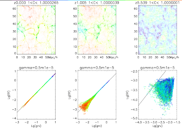
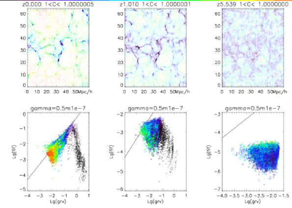
Figure 6: (Color Online) The simulation results for the $\gamma=0.5$ and $\mu=10^{-5},10^{-7}$ runs at redshifts $z=0$, $z=1$, and $z=5.5$. Shown are the particle spatial yz distribution in a slab of $x=31.5-32.5$Mpc/h (upper panel) and the lg-lg diagram of the fifth force vs. gravity in this slab (lower panel). See text for a detailed description. Each particle is a symbol with its color denoting the the value of the effective mass $C(\varphi)$, whose minimum/maximimu are given on top of each panel, and correspond to the two ends of the color scale shown on the top. The size of square symbols in lower panels are proportional to the mis-alignment angle between the fifth force and the gravity on a particle; the biggest squares correspond to anti-alignment, and particles with well-aligned forces are shown as dots. A line showing a fifth-to-gravity ratio of $2\gamma^{2}$ is also drawn to show the (lack of) correlations of the two forces. Note that $C(\varphi)$ is generally the biggest in voids where the forces are the weakest, poorly aligned and less-correlated.

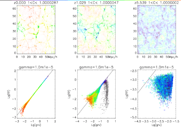
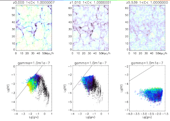
Figure 7: (Color Online) The same as Fig. 6 but for the $\gamma=1.0$ and $\mu=10^{-5},10^{-7}$ runs.

In Figs. 6, 7 we have shown the results for the runs with $\gamma=0.5,1.0$ and $\mu=10^{-5},\mu^{-7}$. These choices of $\mu$ are such that for $\mu=10^{-7}$ (the lower two rows) the chameleon effect is pretty strong while for $\mu=10^{-5}$ (the upper two rows) it is much weaker; the choices of $\gamma$ are to see the effects of different full strengths of the fifth force. The three panels in the first and third rows display the particle distributions at three output redshifts $z\doteq 5.5,~{}1.0,~{}0.0$ from right to left, and the three panels in the second and fourth rows show the correlation between the fifth force and gravity at these redshifts.

For clearness we have only plotted a thin slice (along the $x$ direction) of the full 3-dimensional particle distribution. First let’s have a look at the first and third rows. Because we have output the scalar field value at the position of each particle together with other parameters of the particle, we also include this information in the plots. On top of each panel the range of the value $C(\varphi)$ at the positions of all the shown particles is shown, and color is used to illustrate the amplitude of $C(\varphi)$ (going from black to red from the minimum to the maximum value of $C(\varphi)$). Note that $C(\varphi)=\exp(\gamma\sqrt{\kappa}\varphi)\doteq 1+\gamma\sqrt{\kappa}\varphi$ for $\sqrt{\kappa}\varphi\ll 1$, thus the color also indicates the value of the scalar field indirectly. Also bear in mind that the same color may denote different values of $C(\varphi)$ at different redshifts. The scalar field or $C(\varphi)$ grows with time in general.

Next look at the second and fourth rows, which display the logarithmic of the magnitude of the fifth force versus that of gravity. The color here has the same meaning as above. Furthermore, each point (particle) now is engaged with a square box centered on it, which denotes the size of the angle (from $0$ to $\pi$) between the two forces; the size of the box increases linearly with the angle, from a minimum size $0$ to a maximum size comparable to the largest box size shown in the entire figure. As we have mentioned above, the strength of the fifth force, if not suppressed by the chameleon mechanism, is $2\gamma^{2}$ times that of gravity, so we also plot the functions

$$\lg F = \lg G+\lg(2\gamma^{2}),$$ (55)

where $F,G$ are respectively the magnitudes of the fifth force and gravity, as the black solid lines in these figure, to compare with the simulation data.

We can understand these results qualitatively as follows by taking Fig. 6 as example. The chameleon effect is generally stronger at earlier times when matter density is high and the scalar field value is small. As is shown in the panels of the first row, at redshift $z=5.5$ there is a strong contrast of the value $C(\varphi)$ in high density (blue) regions (clusters hereafter) compared to $C(\varphi)$ in the low density (green, yellow and red) regions (voids hereafter), which is a direct reflection of the nonlinearity in the scalar field. As time evolves and the background value of the scalar field increases, at redshift $z=1.0$ the chameleon effect gets suppressed; this is manifested by the facts that (1) in the regions of small clusters the scalar field values are no longer significantly different from the background value, both of which are yellow and orange-colored, (2) even in the largest clusters the contrast between the scalar field values inside and outside (green/light blue versus yellow/orange) is not so strong compared with the result at redshift $z=5.5$ (purple/dark blue versus green/yellow). These show that the size of nonlinear regions is shrinking and the thin shells in the clusters are thickening, together leading to less nonlinear behaviors of the scalar field. At redshift $z=0.0$ this tendency just becomes more obvious, leaving only a small portion of the space with chameleon effect and thin shells.

The strength of the chameleon effect is determined by several factors. In principle, the larger the effective mass of scalar field ($m_{eff}$) at a position is, the shorter-ranged the fifth force is and the less sensitive the scalar field value at this position will be to the matter distribution around it: this in turn corresponds to a stronger chameleon effect because the scalar field value is mainly determined by the local matter density. On the other hand, $m_{eff}$ depends on $\mu$ (smaller $\mu$ implies larger $m_{eff}$ within a given cluster and thus stronger chameleon effect), $\gamma$ and local $\rho_{\mathrm{CDM}}$ (larger values for these two parameters also imply larger $m_{eff}$ and stronger chameleon effect) and also the background value of the scalar field (this is because the interior solution of the scalar field inside a cluster should only be solved given the boundary conditions outside the cluster, due to the differential nature of the scalar field EOM. Of course for very small $\mu$ and/or very large $\gamma$, the scalar field EOM indeed behaves as an algebraic equation and then the influence of the background value of the scalar field is not important, but for our choices of $\mu,\gamma$ that influence is significant). These analysis agree well with what we have seen in the scalar field configuration from the above N-body simulation results (first and third rows of Fig. 6). Also note that the fifth force is much weaker in regions where chameleon effect is strong, because a particle there can only feel the fifth force from those particles that are very close to it: in this sense we say that the chameleon effect could suppress the fifth force.

A comparison between gravity and the fifth force can illustrate this more clearly. Remember that the chameleon effect could strongly suppress the fifth force. At low redshift ($z=0.0$) the chameleon effect is not significant and so the fifth force is not suppressed; in this case we find that there is a strong correlation between both the magnitudes and directions of these two forces, and the simulation results agree with the prediction Eq. (55) to very high degrees. Both forces are stronger in clusters and weaker in voids as expected. Going backwards in time to the redshift $z=1.0$, there is still a good correlation but the simulation results begin to scatter over the predicted line Eq. (55) in the void regions due to the chameleon effect (the scalar field potential term in Eq. (49) becomes comparable with the matter coupling term). Finally, at very early times ($z=5.5$) the scalar field value becomes so small that the potential term in Eq. (49) is indeed much more important than the matter coupling term so that the latter can be neglected: we then have a complete mismatch between the numerical results and the prediction Eq. (55) as almost all data points are significantly below the black solid line.

The above mismatch in the strongly chameleon regime can be understood schematically as follows:

1. When there is no potential for the scalar field but just a matter coupling, the fifth force is indeed long ranged and can probe the same region as gravity does. Then a comparison of Eqs. (47, 48, 49) shows that the fifth force is exactly $2\gamma^{2}$ times of gravity. This is indeed what we have observed for $z=0.0$ when the potential term in Eq. (49) is negligible.

2. When the scalar field has a potential, it acquires an effective mass which is well-known to be inversely proportional to the range of the scalar fifth force. As a result the fifth force is no longer as long range as gravity. Meanwhile, Eq. (47) makes it clear that the scalar field $\varphi$ (or equivalently $\ln[C(\varphi)]$) acts as a potential for the fifth force, and Eq. (49) shows that this potential depends on the underlying matter distribution in a different (nonlinear) way from what the gravitational potential $\Phi$ does.

   So we could see that there will be differences between both the ranges and the magnitudes of gravity and fifth force. In high density regions these differences will be dominated over by the competing effects that (i) the majority part of the (either gravitational or fifth) force on a particle is contributed by nearby particles and there are so many particles nearby that contribution from distant particles is negligible, (ii) in Eq. (49) the potential term is much less important than the matter coupling term, together making the fifth force behavior similar to that of gravity again. In the void regions the number of nearby particles is small so that contribution from distant particles should be taken into account, and the matter coupling term in Eq. (49) is much smaller, then the difference between gravity and the fifth force becomes manifesting. These effects can be observed in the $z=1.0$ panel.

3. At even higher redshifts the potential of the scalar field makes its effective mass very large and thus its range very short compared with that of gravity. Meanwhile Eq. (49) becomes very nonlinear due to the smallness of the scalar field value, and thus the fifth force potential depends on matter distribution very differently from the gravitational potential.

   As a result, the fifth force reflects the matter distribution in a very small region around a given particle, while gravity probes that in a much larger region. Even in that small region where both forces exist, their magnitude can generally be very different. So it is not surprising that the two forces look so different as in the $z=5.5$ panel. Note that here the fifth force is also much weaker than gravity because its strength is suppressed by the smallness of the scalar field value.

Result for the $\mu=10^{-7}$ case (the lower two rows) is qualitatively the same as that of the $\mu=10^{-5}$ case above, but here because $\mu$ is much smaller, so the chameleon effect exists until much more recent than in the $\mu=10^{-5}$ case. Indeed, even at low redshifts $z=1.0$ and $0.0$ there is still strong contrast between the scalar field values inside and outside the clusters (purple/dark blue versus yellow/orange). The correlation between the forces also follow our above analysis, but here there are some new features. The first feature is that even today the fitting to Eq. (55) is far from perfect; this is easy to understand, because the scalar field potential is so nonlinear that the scalar field potential term in Eq. (49) is important up to now. The second feature is that in the $z=0.0$ (also $z=1.0$) panel we could find that in high density regions the fifth force does not obey Eq. (55) as in the $\mu=10^{-5}$ case, but becomes much smaller than gravity – actually, the stronger gravity is, the weaker the fifth force will be! This is again due to the strong chameleon effect in the clusters, which makes the scalar field value very small and thus suppresses the fifth force there. Note that this feature is desirable because if we also couple the scalar field to baryonic matter then we definitely want the fifth force to be suppressed to evade solar system tests.

If we choose $\gamma=1.0$ as in Fig. 7, then all the qualitative results we have obtained above should still apply. But the stronger coupling between matter and the scalar field enhances the chameleon effect. This implies that a coupling whose strength is significantly larger than that of gravity could probably produce the correct amount of large scale structure as observed by suppressing the fifth force on all cosmological epochs and scales of interests to us.

The analysis above clearly shows the complexity of the fifth force and its possible effects on the nonlinear structure formation. Though in certain (no chameleon) limits the fifth force is greatly simplified and one can assume a modified gravitational constant in the N-body simulations as an approximation, this is evidently not the case if the scalar field potential is too much nonlinear. Of course, we have no a priori knowledge about when the chameleon effect becomes important, and full numerical simulations like the one presented here are therefore necessary to precisely study the effects of (coupled) scalar fields in the large scale structure. In forthcoming works we shall analyze the nonlinear matter power spectrum, halo profile, scalar field configuration within clusters, as well as the development and disappearance of thin shells in a quantitative manner.

One may wonder if a more complete simulation should keep the time derivatives of the scalar field in Eq. (IV.1). This is certainly true, yet these terms indeed have negligible effect Oyaizu (2008), which could be understood in the following way: when there is no (or very weak) chameleon effect, the scalar field potential term in Eq. (49) is negligible and so this equation has the same form as the Poisson equation Eq. (48); as a result the quasi-static approximation works as well for the scalar field as for the gravitational potential (which is what any N-body code relies on). On the other hand, if there is strong chameleon effect, the scalar field value tends to be much smaller which means that the time derivative of the scalar field also gets smaller; and at the same time the spatial gradient of the scalar field becomes larger: these together indicate that the quasi-static approximation should be good here too.

V Conclusion

To conclude, in this paper we have presented the general frameworks to study the linear and nonlinear structure formations in coupled scalar field models, and given some preliminary numerical results for both in the context of a specific coupling function and scalar field potential.

For the linear large scale structure, we write down the perturbed field equations using the $3+1$ decomposition, which can be directly applied into numerical Boltzmann codes such as CAMB to generate the CMB and matter power spectra. For the chosen coupling function with parameter $\gamma$ and potential with parameter $\mu$, we find that $\gamma$ roughly controls the strength of the fifth force (which is due to the propagation of the scalar field) while $\mu$ controls how much the effect of the fifth force is suppressed by the chameleon mechanism. With $\mu\lesssim\mathcal{O}(0.1)$ the chameleon effect makes the model behave like $\Lambda$CDM on very large scales, but this is far from enough to significantly decrease the effects of the fifth force on the small scale density perturbation growth. On those small scales, however, nonlinearity becomes an important issue, which leads us to the N-body simulation in § IV.

Previous N-body simulations with scalar fields are generally simplified by certain approximations such as treating the scalar coupling effect as a simple change of gravitational constant $G$, or assuming a Yukawa-type force with a certain range. These approximations do not work well in the present model, and so here we set up the formula needed for a more precise simulation, putting much emphasis on the calculation of the fifth force and its action on particles. The equations derived and the algorithm described in § IV are general enough and should be directly applicable to other coupled scalar field models.

We integrate the equations into a modified version of the N-body code MLAPM and performed several runs with different combinations of $\gamma,\mu$. Some results are displayed in Figs. 6 and 7. It is confirmed that when the chameleon effect is not important, the fifth force is parallel to gravity and is $2\gamma^{2}$ times stronger, meaning that simply using a different gravitational constant which is $2\gamma^{2}+1$ times as large as the bare one in the simulation should be an acceptable approximation. There are some caveats however. For one thing, the correlation between gravity and the fifth force is only good for a portion of the parameter space $(\gamma,\mu)$, and for $\mu\ll 1$ the potential is so nonlinear as to destroy this correlation. More importantly, even the correlation is perfect now it is possible that at earlier times the nonlinear effects modify it dramatically (cf. Fig. 7 with $\mu=10^{-5}$ at $z=0.0,1.0$). This means that the above-mentioned approximation is unlikely to be correct consistently and full simulations as the ones in this paper are needed.

All in all, from the results we can spot the trend that, with the same value of $\mu$ increasing $\gamma$ simply enhances the power of structure growth, while with the same value of $\gamma$ decreasing $\mu$ has the effects of reducing that power. Also, for small $\mu$ the configuration of the scalar field becomes very nonlinear and highly sensitive to the underlying matter distribution, while for large $\mu$ this becomes much more smooth and stiff. All these observations (and others as explained in § IV.4) agree with the chameleon analysis. Our simulations also provides a test bed for scalar field theories. Among the applications, one could look for high-speed encounters of halos to see the probability of generating a Bullet-cluster-like encounters Springel (2007); Claudio (2009). Since this paper is only served to set up the general framework of linear and nonlinear simulations, these applications of the simulation results, as well as the matter power spectrum and scalar field profile/evolution, will be presented in forthcoming works.

Appendix A The Perturbation Equations

Consider the decomposition of the stress energy tensor $T_{ab}$

$$T_{ab} = \pi_{ab}+2q_{(a}u_{b)}+\rho u_{a}u_{b}-ph_{ab}$$ (56)

where $u_{a}$ is the 4-velocity of an observer with respect to which $3+1$ space-time splitting is made, $h_{ab}=g_{ab}-u_{a}u_{b}$ the projection tensor used to obtain covariant tensors perpendicular to $u_{a}$. Here $\pi_{ab}$ is the projected symmetric tracefree anisotropic stress, $q$ is the vector heat flux and $\rho$ and $p$ respectively the energy density and isotropic pressure. These quantities could be obtained from $T_{ab}$ through the relations

$$\rho = T_{ab}u^{a}u^{b},$$

$$p = -\frac{1}{3}h^{ab}T_{ab},$$

$$q_{a} = h^{d}_{a}u^{c}T_{cd},$$

$$\pi_{ab} = h^{c}_{a}h^{d}_{b}T_{cd}+ph_{ab}.$$ (57)

Based on these, the components of the stress energy tensor (up to first order) in this model is summarized in the following table:

Table 1: The decomposition of energy momentum tensor in the $3+1$ formalism.

Matter	$\rho$	$p$	$q_{a}$	$\pi_{ab}$
$\gamma$	$\rho_{\gamma}$	$\frac{1}{3}\rho_{\gamma}$	$q_{\gamma a}$	$\pi_{\gamma ab}$
$\nu$	$\rho_{\nu}$	$\frac{1}{3}\rho_{\nu}$	$q_{\nu a}$	$\pi_{\nu ab}$
Baryons	$\rho_{\mathrm{B}}$	$p_{\mathrm{B}}$	$q_{\mathrm{B}a}$	$0$
CDM	$\rho_{\mathrm{CDM}}$	$0$	$q_{\mathrm{CDM}a}$	$0$
Coupled CDM	$C(\varphi)\rho_{\mathrm{CDM}}$	$0$	$C(\varphi)q_{\mathrm{CDM}a}$	$0$
$\varphi$	$\frac{1}{2}\dot{\varphi}^{2}+V(\varphi)$	$\frac{1}{2}\dot{\varphi}^{2}-V(\varphi)$	$\dot{\varphi}\hat{\nabla}_{a}\varphi$	$0$

Throughout this paper an overdot denotes the derivative with respect to the cosmic time $t$ and $\hat{\nabla}_{a}$ is the covariant spatial derivative perpendicular to $u_{a}$ (up to first order in perturbation). Note that it is the coupled CDM quantities which appear in the (background and perturbed) Einstein equations, and also note that we have included the massless neutrinos into the model here.

The five constraint equations in the model are given as

$$0 = \hat{\nabla}^{c}(\epsilon_{\ \ cd}^{ab}u^{d}\varpi_{ab});$$ (58)

$$\kappa q_{a} = -\frac{2\hat{\nabla}_{a}\theta}{3}+\hat{\nabla}^{b}\sigma_{ab}+\hat{\nabla}^{b}\varpi_{ab};\ \ \$$ (59)

$$\mathcal{B}_{ab} = \left[\hat{\nabla}^{c}\sigma_{d(a}+\hat{\nabla}^{c}\varpi_{d(a}\right]\epsilon_{b)ec}^{\ \ \ \ d}u^{e};$$ (60)

$$\hat{\nabla}^{b}\mathcal{E}_{ab} = \frac{1}{2}\kappa\left[\hat{\nabla}^{b}\pi_{ab}+\frac{2}{3}\theta q_{a}+\frac{2}{3}\hat{\nabla}_{a}\rho\right];$$ (61)

$$\hat{\nabla}^{b}\mathcal{B}_{ab} = \frac{1}{2}\kappa\left[\hat{\nabla}_{c}q_{d}+(\rho+p)\varpi_{cd}\right]\epsilon_{ab}^{\ \ cd}u^{b}.$$ (62)

Here, $\epsilon_{abcd}$ is the covariant permutation tensor, $\mathcal{E}_{ab}$ and $\mathcal{B}_{ab}$ are respectively the electric and magnetic parts of the Weyl tensor $\mathcal{W}_{abcd}$, given respectively through $\mathcal{E}_{ab}=u^{c}u^{d}\mathcal{W}_{acbd}$ and $\mathcal{B}_{ab}=-\frac{1}{2}u^{c}u^{d}\epsilon_{ac}^{\ \ ef}\mathcal{W}_{efbd}$. $\theta,\sigma_{ab},\varpi_{ab}$ come from the decomposition of the covariant derivative of 4-velocity

$$\nabla_{a}u_{b} = \sigma_{ab}+\varpi_{ab}+\frac{1}{3}\theta h_{ab}+u_{a}A_{b}$$ (63)

with $A$ being the acceleration, $\theta=\nabla^{c}u_{c}=3\dot{a}/a$ the expansion scalar, $\varpi_{ab}=\hat{\nabla}_{[a}u_{b]}$ and $\sigma_{ab}$ the shear. Note that $\theta$ in the above section has a completely different meaning.

In addition, the seven propagation equations are:

$$\dot{\rho}+(\rho+p)\theta+\hat{\nabla}^{a}q_{a} = 0;$$ (64)

$$\dot{q}_{a}+\frac{4}{3}\theta q_{a}+(\rho+p)A_{a}-\hat{\nabla}_{a}p+\hat{\nabla}^{b}\pi_{ab} = 0;$$

$$\dot{q}_{a}+\frac{4}{3}\theta q_{a}+(\rho+p)A_{a}-\hat{\nabla}_{a}p+\hat{\nabla}^{b}\pi_{ab}$$

$$-\frac{C_{\varphi}}{C}(\rho_{\mathrm{CDM}}\hat{\nabla}_{a}\varphi-\dot{\varphi}q_{\mathrm{CDM}a}) = 0;$$ (65)

$$\dot{\theta}+\frac{1}{3}\theta^{2}-\ \hat{\nabla}^{a}A_{a}+\frac{\kappa}{2}(\rho+3p) = 0;$$ (66)

$$\dot{\sigma}_{ab}+\frac{2}{3}\theta\sigma_{ab}-\hat{\nabla}_{\langle a}A_{b\rangle}+\mathcal{E}_{ab}+\frac{1}{2}\kappa\pi_{ab} = 0;$$ (67)

$$\dot{\varpi}+\frac{2}{3}\theta\varpi-\hat{\nabla}_{[a}A_{b]} = 0;$$ (68)

$$\frac{1}{2}\kappa\left[\dot{\pi}_{ab}+\frac{1}{3}\theta\pi_{ab}\right]-\frac{1}{2}\kappa\left[(\rho+p)\sigma_{ab}\ +\hat{\nabla}_{\langle a}q_{b\rangle}\right]$$

$$-\left[\dot{\mathcal{E}}_{ab}+\theta\mathcal{E}_{ab}-\hat{\nabla}^{c}\mathcal{B}_{d(a}\epsilon_{b)ec}^{\ \ \ \ d}u^{e}\right] = 0;$$ (69)

$$\dot{\mathcal{B}}_{ab}+\theta\mathcal{B}_{ab}+\hat{\nabla}^{c}\mathcal{E}_{d(a}\epsilon_{b)ec}^{\ \ \ \ d}u^{e}+\frac{1}{2}\kappa\hat{\nabla}^{c}\mathcal{\pi}_{d(a}\epsilon_{b)ec}^{\ \ \ \ d}u^{e} = 0.\ \ \ \$$ (70)

where the angle bracket means taking the trace-free part of a quantity. Note that the first of Eq. (A) is for normal matter while the second is for the coupled dark matter.

Besides the above equations, it is useful to express the projected Ricci scalar $\hat{R}$ into the hypersurfaces orthogonal to $u^{a}$ as

$$\hat{R} \doteq 2\kappa\rho-\frac{2}{3}\theta^{2}.$$ (71)

The spatial derivative of the projected Ricci scalar, $\eta_{a}\equiv\frac{1}{2}a\hat{\nabla}_{a}\hat{R}$, is given as

$$\eta_{a} = a\kappa\hat{\nabla}_{a}\rho-\frac{2a}{3}\theta\hat{\nabla}_{a}\theta,$$ (72)

and its propagation equation

$$\dot{\eta}_{a}+\frac{2\theta}{3}\eta_{a} = -\frac{2a}{3}\theta\hat{\nabla}_{a}\hat{\nabla}^{b}A_{b}-a\kappa\hat{\nabla}_{a}\hat{\nabla}^{b}q_{b}.$$ (73)

As we are considering a spatially flat universe, the spatial curvature must vanish on large scales which means that $\hat{R}=0$. Thus, from Eq. (71), we can obtain the Friedman equation

$$\frac{1}{3}\theta^{2} = \kappa\rho.$$ (74)

Note that in all the above equations $\rho,\ p,\ q_{a}$ and $\pi_{ab}$ are all the total quantities contributed by all matter species:

$$\rho = \rho_{\gamma}+\rho_{\nu}+\rho_{\mathrm{B}}+C(\varphi)\rho_{\mathrm{CDM}}+\frac{1}{2}\dot{\varphi}^{2}+V(\varphi),$$

$$p = \frac{1}{3}\rho_{\gamma}+\frac{1}{3}\rho_{\nu}+p_{\mathrm{B}}+\frac{1}{2}\dot{\varphi}^{2}-V(\varphi),$$

$$q_{a} = q_{\gamma a}+q_{\nu a}+q_{\mathrm{B}a}+C(\varphi)q_{\mathrm{CDM}a}+\dot{\varphi}\hat{\nabla}_{a}\varphi,$$

$$\pi_{ab} = \pi_{\gamma ab}+\pi_{\nu ab}.$$ (75)

Finally, there is the perturbed scalar field EOM

$$\ddot{\varphi}+\theta\dot{\varphi}+\hat{\nabla}^{2}\varphi+\frac{\partial V(\varphi)}{\partial\varphi}+\rho_{\mathrm{CDM}}\frac{\partial C(\varphi)}{\partial\varphi} = 0.$$ (76)

Appendix B Equations in $k$ Space

To put the above perturbation equations into numerical calculation, we need to write them in the $k$-space. As we want to present the complete framework to study the structure formation in coupled scalar field models, here we also list those equations.

First of all, the change into $k$-space is accomplished with the aid of following Harmonic expansions:

$$\mathcal{X}_{a}\equiv a\hat{\nabla}_{a}\rho=\sum_{k}k\mathcal{X}Q^{k}_{a}\ \ \ \ \ q_{a}=\sum_{k}qQ^{k}_{a}\ \ \ \$$

$$\pi_{ab}=\sum_{k}\Pi Q^{k}_{ab}\ \ \ \ \ \mathcal{Z}_{a}\equiv a\hat{\nabla}_{a}\theta=\sum_{k}\frac{k^{2}}{a}\mathcal{Z}Q^{k}_{a}\ \ \ \$$

$$\sigma_{ab}=\sum_{k}\frac{k}{a}\sigma Q^{k}_{ab}\ \ \ \ \ \eta_{a}=\sum_{k}\frac{k^{3}}{a^{2}}\eta Q^{k}_{a}$$

$$h_{a}\equiv\hat{\nabla}_{a}a=\sum_{k}khQ^{k}_{a}\ \ \ \ \ A_{a}=\sum_{k}\frac{k}{a}AQ^{k}_{a}\ \ \ \$$

$$\mathcal{E}_{ab}=-\sum_{k}\frac{k^{2}}{a^{2}}\phi Q^{k}_{ab}\ \ \ \ \ \hat{\nabla}_{a}\varphi=\sum_{k}\frac{k}{a}\xi Q^{k}_{a}$$ (77)

where $Q^{k}_{a}=\frac{a}{k}\hat{\nabla}_{a}Q^{k}$ with $Q^{k}$ being the zero order eigenfunctions of the comoving Laplacian $a^{2}\hat{\nabla}^{2}$ ($a^{2}\hat{\nabla}^{2}Q^{k}=k^{2}Q^{k}$) and $Q^{k}_{ab}=\frac{a}{k}\hat{\nabla}_{\langle a}Q^{k}_{b\rangle}$. Note that we only consider scalar mode perturbations in the present paper and so shall neglect the second order quantities such as $\mathcal{B}_{ab}$ and $\varpi_{ab}$.

With these we list the equations that will be used in the numerical calculation of the linear large scale structure.

B.0.1 Background Evolution for Energy Densities

$$\rho_{\gamma}^{\prime}+4\frac{a^{\prime}}{a}\rho_{\gamma} = 0,$$ (78)

$$\rho_{\nu}^{\prime}+4\frac{a^{\prime}}{a}\rho_{\nu} = 0,$$ (79)

$$\rho_{\mathrm{B}}^{\prime}+3\frac{a^{\prime}}{a}\rho_{\mathrm{B}} = 0,$$ (80)

$$\rho_{\mathrm{CDM}}^{\prime}+3\frac{a^{\prime}}{a}\rho_{\mathrm{CDM}} = 0.$$ (81)

Note that because our definition of the dark matter energy density includes only the mass density, but not the contribution from its coupling to the scalar field, so $\rho_{\mathrm{CDM}}$ evolves as in $\Lambda$CDM. One can also understand this as follows: the coupling to the scalar field produces a fifth force on the dark matter particles, making their trajectories be non-geodesic, but as we shall see below, the fifth force is spatial (perpendicular to the worldline of the dark matter particle) and cannot change the mass of dark matter particles. Consequently the averaged dark matter mass density is the same as in $\Lambda$CDM. One can of course define the energy momentum tensor for dark matter as including $C(\varphi)$, and in this case Eq. (81) will no longer be valid and we end up with varying mass dark matter particles.

B.0.2 Propagations of Spatial Gradients of Densities

$$\Delta^{\prime}_{\gamma}+\frac{4}{3}k\mathcal{Z}-4\frac{a^{\prime}}{a}A+kv_{\gamma} = 0,$$ (82)

$$\Delta^{\prime}_{\nu}+\frac{4}{3}k\mathcal{Z}-4\frac{a^{\prime}}{a}A+kv_{\nu} = 0,$$ (83)

$$\Delta^{\prime}_{\mathrm{B}}+\left(k\mathcal{Z}-3\frac{a^{\prime}}{a}A+kv_{{}_{\mathrm{B}}}\right)+3\frac{a^{\prime}}{a}c^{2}_{s}\Delta_{\mathrm{B}} = 0,$$ (84)

$$\Delta^{\prime}_{\mathrm{CDM}}+k\mathcal{Z}-3\frac{a^{\prime}}{a}A+kv_{\mathrm{CDM}} = 0.$$ (85)

B.0.3 Propagations of Heat Fluxes

$$v^{\prime}_{\nu}+\frac{k}{3}\left(2\frac{\Pi_{\nu}}{\rho_{\nu}}+4A-\Delta_{\nu}\right) = 0,$$ (86)

$$v^{\prime}_{\gamma}+\frac{k}{3}\left(2\frac{\Pi_{\gamma}}{\rho_{\gamma}}+4A-\Delta_{\gamma}\right)$$

$$+an_{e}\sigma_{\mathrm{T}}\left(v_{\gamma}-\frac{4}{3}v_{\mathrm{B}}\right) = 0,$$ (87)

$$v^{\prime}_{\mathrm{B}}+\frac{a^{\prime}}{a}(1-3c^{2}_{s})v_{\mathrm{B}}+kA$$

$$-kc^{2}_{s}\Delta_{\mathrm{B}}+an_{e}\sigma_{\mathrm{T}}\frac{\rho_{\gamma}}{\rho_{\mathrm{B}}}\left(\frac{4}{3}v_{\mathrm{B}}-v_{\gamma}\right) = 0,$$ (88)

$$v^{\prime}_{\mathrm{CDM}}+\frac{a^{\prime}}{a}v_{\mathrm{CDM}}+kA+\frac{C_{\varphi}}{C}\varphi^{\prime}v_{\mathrm{CDM}}-\frac{C_{\varphi}}{C}k\xi = 0.$$ (89)

B.0.4 Other Propagation Equations

$$k\left(\sigma^{\prime}+\frac{a^{\prime}}{a}\sigma\right)-k^{2}\left(A+\phi\right)+\frac{1}{2}\kappa\Pi a^{2} = 0,$$ (90)

$$k^{2}\left(\phi^{\prime}+\frac{a^{\prime}}{a}\phi\right)$$

$$+\frac{1}{2}\kappa\left[\Pi^{\prime}+\frac{a^{\prime}}{a}\Pi-k(\rho+p)\sigma-kq\right]a^{2} = 0,$$ (91)

$$k\eta^{\prime}+2\frac{a^{\prime}}{a}kA+\kappa qa^{2} = 0,$$ (92)

in which we have used

$$\rho = \rho_{\gamma}+\rho_{\nu}+\rho_{\mathrm{B}}+C(\varphi)\rho_{\mathrm{CDM}}+\frac{1}{2a^{2}}\varphi^{\prime 2}+V(\varphi),\ \ \ \$$ (93)

$$p = \frac{1}{3}\rho_{\gamma}+\frac{1}{3}\rho_{\nu}+\frac{1}{2a^{2}}\varphi^{\prime 2}-V(\varphi),$$ (94)

$$q = \rho_{\gamma}v_{\gamma}+\rho_{\nu}v_{\nu}+\rho_{\mathrm{B}}v_{\mathrm{B}}+\frac{k}{a^{2}}\varphi^{\prime}\xi,\ \$$ (95)

$$\Pi = \Pi_{\gamma}+\Pi_{\nu},$$ (96)

$$\mathcal{X} = \rho_{\gamma}\Delta_{\gamma}+\rho_{\nu}\Delta_{\nu}+\rho_{{}_{\mathrm{B}}}\Delta_{{}_{\mathrm{B}}}+C(\varphi)\rho_{{}_{\mathrm{CDM}}}\Delta_{{}_{\mathrm{CDM}}}$$ (97)

$$+\frac{1}{a^{2}}\varphi^{\prime}\xi^{\prime}+\left(\frac{1}{a^{2}}\frac{C_{\varphi}}{C}\varphi^{\prime 2}+V_{\varphi}+C_{\varphi}\rho_{\mathrm{CDM}}\right)\xi\ \$$

and defined the density contrast $\Delta_{i}=\mathcal{X}_{i}/\rho_{i}$ for matter species $i$.

B.0.5 Constraint Equations

$$k^{2}(\mathcal{Z}-\sigma)+\frac{3}{2}\kappa qa^{2} = 0,$$ (98)

$$k^{3}\phi+\frac{1}{2}\kappa\left[k(\Pi+\mathcal{X})+3\frac{a^{\prime}}{a}q\right]a^{2} = 0,$$ (99)

$$k^{2}\eta+2\frac{a^{\prime}}{a}k\mathcal{Z}-\kappa\mathcal{X}a^{2} = 0.$$ (100)

B.0.6 Scalar Field Equations of Motion

$$\varphi^{\prime\prime}+2\frac{a^{\prime}}{a}\varphi^{\prime}+\frac{\partial V(\varphi)}{\partial\varphi}a^{2}+\rho_{\mathrm{CDM}}\frac{\partial C(\varphi)}{\partial\varphi}a^{2} = 0,$$ (101)

$$\xi^{\prime\prime}+2\frac{a^{\prime}}{a}\xi^{\prime}+\left(k^{2}+a^{2}V_{\varphi\varphi}+a^{2}\rho_{\mathrm{CDM}}C_{\varphi\varphi}\right)\xi$$

$$+\left(2\varphi^{\prime\prime}+\frac{a^{\prime}}{a}\varphi^{\prime}\right)A+a^{2}C_{\varphi}\rho_{\mathrm{CDM}}\Delta_{\mathrm{CDM}}$$

$$+\left(k\mathcal{Z}+A^{\prime}\right)\varphi^{\prime} = 0.$$ (102)

B.0.7 The Friedmann Equations

$$3\left(\frac{a^{\prime}}{a}\right)^{2} = \kappa\rho a^{2},$$ (103)

$$\frac{a^{\prime\prime}}{a}-\left(\frac{a^{\prime}}{a}\right)^{2} = -\frac{\kappa}{6}(\rho+3p)a^{2}.$$ (104)

When it comes to perturbation calculations, we need to fix a gauge, i.e., choose a $u_{a}$. One possibility is to use the 4-velocity of dark matter particles as our $u_{a}$. In this case the dark matter heat flux is zero and according to Eq. (89) we will simply have $A=\frac{C_{\varphi}}{C}\xi$, and this relation can then be used to replace the $A$’s appearing in all the above equations. Another possibility is to choose $u_{a}$ such that $A=0$: in this case $v_{\mathrm{CDM}}$ will become nonzero and we need to dynamically evolve it. Below in the numerical calculations we shall adopt the second possibility.

Appendix C Discretized Equations for N-body Simulations Non-linear Regime

In the MLAPM code the partial differential equation Eq. (48) is (and in our modified code Eq. (49) will also be) solved on discretized grid points, and as such we must develop the discretized versions of Eqs. (46 - 49) to be implemented into the code.

But before going on to the discretization, we need to address a technical issue. As the potential is highly nonlinear, in the high density regime the value of the scalar field $\sqrt{\kappa}\varphi$ will be very close to 0, and this is potentially a disaster as during the numerical solution process the value of $\sqrt{\kappa}\varphi$ might easily go into the forbidden region $\varphi<0$ Oyaizu (2008). One way of solving this problem is to define $\chi=\bar{\chi}e^{u}$ in which $\bar{\chi}$ is the background value of $\chi$, as in Oyaizu (2008). Then the new variable $u$ takes value in $(-\infty,\infty)$ so that $e^{u}$ is positive definite which ensures that $\chi>0$. However, since there are already exponentials of $\chi$ in the potential, this substitution will result terms involving $\exp\left[\exp(u)\right]$, which could potentially magnify any numerical error in $u$.

Instead, we can define a new variable $u$ according to

$$e^{u}+1 = e^{\chi}.$$ (105)

By this, $u$ still takes value in $(-\infty,\infty)$, $e^{u}\in(0,\infty)$ and thus $e^{\chi}\in(1,\infty)$ which ensures that $\chi$ is positive definite in numerical solutions. Besides, $e^{\beta\chi}=\left[1+e^{u}\right]^{\beta}$ so that there will be no exponential-of-exponential terms, and the only exponential is what we have for the potential itself. $\beta=-1$ above.

Then the Poisson equation becomes

$$\nabla^{2}\Phi_{c} = \frac{3}{2}\Omega_{\mathrm{CDM}}\left[\rho_{c}\left(1+e^{u}\right)^{\gamma}-e^{\gamma\sqrt{\kappa}\bar{\varphi}}\right]$$ (106)

$$-\frac{3\Omega_{V_{0}}a^{3}}{\left[1-\left(1+e^{u}\right)^{\beta}\right]^{\mu}}+3\bar{\Omega}_{V}a^{3},$$

where we have defined $\bar{\Omega}_{V}=\kappa V(\bar{\varphi})/3H_{0}^{2}$ which is determined by background cosmology, the quantity $e^{\gamma\sqrt{\kappa}\bar{\varphi}}$ is also determined solely by background cosmology. These background quantities should not bother us here.

The scalar field EOM becomes

$$\frac{ac^{2}}{\left(H_{0}B\right)^{2}}\nabla\cdot\left(\frac{e^{u}}{1+e^{u}}\nabla u\right)$$ (107)

$$= 3\gamma\Omega_{\mathrm{CDM}}\rho_{c}\left(1+e^{u}\right)^{\gamma}+\frac{3\mu\beta\Omega_{V_{0}}a^{3}\left(1+e^{u}\right)^{\beta}}{\left[1-\left(1+e^{u}\right)^{\beta}\right]^{\mu+1}}$$

$$-3\gamma\Omega_{\mathrm{CDM}}e^{\gamma\sqrt{\kappa}\bar{\varphi}}-\frac{3\mu\beta\Omega_{V_{0}}a^{3}e^{\beta\sqrt{\kappa}\bar{\varphi}}}{\left[1-e^{\beta\sqrt{\kappa}\bar{\varphi}}\right]^{m+1}}$$

in which we have used the fact that $\chi=\log(1+e^{u})\Rightarrow\nabla\chi=\frac{e^{u}}{1+e^{u}}\nabla u$, and moved all terms depending only on background cosmology (the source terms) to the right hand side.

So, in terms of the new variable $u$, the set of equations used in the N-body code should be

$$\frac{d\mathbf{x}_{c}}{dt_{c}} = \frac{\mathbf{p}_{c}}{a^{2}},$$ (108)

$$\frac{d\mathbf{p}_{c}}{dt_{c}} = -\frac{1}{a}\nabla\Phi_{c}-\frac{c^{2}\gamma}{\left(H_{0}B\right)^{2}}\frac{e^{u}}{1+e^{u}}\nabla u$$ (109)

plus Eqs. (106, 107). These equations will ultimately be used in the code. Among them, Eqs. (106, 109) will use the value of $u$ while Eq. (107) solves for $u$. In order that these equations can be integrated into MLAPM, we need to discretize Eq. (107) for the application of Newton-Gauss-Seidel iterations.

To discretize Eq. (107), let us define $b\equiv\frac{e^{u}}{1+e^{u}}$. The discretization involves writing down a discretion version of this equation on a uniform grid with grid spacing $h$. Suppose we require second order precision as is in the standard Poisson solver of MLAPM, then $\nabla u$ in one dimension can be written as

$$\nabla u \rightarrow \nabla^{h}u_{j}\ =\ \frac{u_{j+1}-u_{j-1}}{2h}$$ (110)

where a subscript _j means that the quantity is evaluated on the $j$-th point. Of course the generalization to three dimensions is straightforward.

The factor $b$ in $\nabla\cdot\left(b\nabla u\right)$ makes this a standard variable coefficient problem. We need also discretize $b$, and do it in this way (again for one dimension):

$$\nabla\cdot\left(b\nabla u\right) \rightarrow \left(\nabla^{h}b_{j}\right)\cdot\left(\nabla^{h}u_{j}\right)+b_{j}\nabla^{h2}u_{j}$$ (111)

$$= \frac{b_{j+1/2}-b_{j-1/2}}{h}\frac{u_{j+1}-u_{j-1}}{2h}+\frac{b_{j+1/2}+b_{j-1/2}}{2}\frac{u_{j+1}-2u_{j}+u_{j-1}}{h^{2}}$$

$$= \frac{1}{h^{2}}\left[b_{j+\frac{1}{2}}u_{j+1}-u_{j}\left(b_{j+\frac{1}{2}}+b_{j-\frac{1}{2}}\right)+b_{j-\frac{1}{2}}u_{j-1}\right]$$

where we have defined $b_{j+\frac{1}{2}}=\left(b_{j}+b_{j+1}\right)/2$ and $b_{j-\frac{1}{2}}=\left(b_{j-1}+b_{j}\right)/2$. This can be easily generalize to three dimensions as

$$\nabla\cdot\left(b\nabla u\right) \rightarrow \frac{1}{h^{2}}\left[b_{i+\frac{1}{2},j,k}u_{i+1,j,k}-u_{i,j,k}\left(b_{i+\frac{1}{2},j,k}+b_{i-\frac{1}{2},j,k}\right)+b_{i-\frac{1}{2},j,k}u_{i-1,j,k}\right]$$ (112)

$$+\frac{1}{h^{2}}\left[b_{i,j+\frac{1}{2},k}u_{i,j+1,k}-u_{i,j,k}\left(b_{i,j+\frac{1}{2},k}+b_{i,j-\frac{1}{2},k}\right)+b_{i,j-\frac{1}{2},k}u_{i,j-1,k}\right]$$

$$+\frac{1}{h^{2}}\left[b_{i,j,k+\frac{1}{2}}u_{i,j,k+1}-u_{i,j,k}\left(b_{i,j,k+\frac{1}{2}}+b_{i,j,k-\frac{1}{2}}\right)+b_{i,j,k-\frac{1}{2}}u_{i,j,k-1}\right].$$

Then the discrete version of Eq. (107) is

$$L^{h}\left(u_{i,j,k}\right) = 0,$$ (113)

in which

$$L^{h}\left(u_{i,j,k}\right) = \frac{1}{h^{2}}\left[b_{i+\frac{1}{2},j,k}u_{i+1,j,k}-u_{i,j,k}\left(b_{i+\frac{1}{2},j,k}+b_{i-\frac{1}{2},j,k}\right)+b_{i-\frac{1}{2},j,k}u_{i-1,j,k}\right]$$ (114)

$$+\frac{1}{h^{2}}\left[b_{i,j+\frac{1}{2},k}u_{i,j+1,k}-u_{i,j,k}\left(b_{i,j+\frac{1}{2},k}+b_{i,j-\frac{1}{2},k}\right)+b_{i,j-\frac{1}{2},k}u_{i,j-1,k}\right]$$

$$+\frac{1}{h^{2}}\left[b_{i,j,k+\frac{1}{2}}u_{i,j,k+1}-u_{i,j,k}\left(b_{i,j,k+\frac{1}{2}}+b_{i,j,k-\frac{1}{2}}\right)+b_{i,j,k-\frac{1}{2}}u_{i,j,k-1}\right]$$

$$-\frac{\left(H_{0}B\right)^{2}}{ac^{2}}\left[3\gamma\Omega_{\mathrm{CDM}}\rho_{c,i,j,k}\left(1+e^{u_{i,j,k}}\right)^{\gamma}+\frac{3\mu\beta\Omega_{V_{0}}a^{3}\left(1+e^{u_{i,j,k}}\right)^{\beta}}{\left[1-\left(1+e^{u_{i,j,k}}\right)^{\beta}\right]^{\mu+1}}\right]$$

$$+\frac{\left(H_{0}B\right)^{2}}{ac^{2}}\left[3\gamma\Omega_{\mathrm{CDM}}e^{\gamma\sqrt{\kappa}\bar{\varphi}}+\frac{3\mu\beta\Omega_{V_{0}}a^{3}e^{\beta\sqrt{\kappa}\bar{\varphi}}}{\left[1-e^{\beta\sqrt{\kappa}\bar{\varphi}}\right]^{\mu+1}}\right].$$

Then the Newton-Gauss-Seidel iteration says that we can obtain a new (and often more accurate) solution of $u$, $u^{\mathrm{new}}_{i,j,k}$, using our knowledge about the old (and less accurate) solution $u^{\mathrm{old}}_{i,j,k}$ as

$$u^{\mathrm{new}}_{i,j,k} = u^{\mathrm{old}}_{i,j,k}-\frac{L^{h}\left(u^{\mathrm{old}}_{i,j,k}\right)}{\partial L^{h}\left(u^{\mathrm{old}}_{i,j,k}\right)/\partial u_{i,j,k}}.$$ (115)

The old solution will be replaced by the new solution to $u_{i,j,k}$ once the new solution is ready, using the red-black Gauss-Seidel sweeping scheme. Note that

$$\frac{\partial L^{h}(u_{i,j,k})}{\partial u_{i,j,k}} = \frac{1}{2h^{2}}\frac{e^{u_{i,j,k}}}{\left(1+e^{u_{i,j,k}}\right)^{2}}\left[u_{i+1,j,k}+u_{i-1,j,k}+u_{i,j+1,k}+u_{i,j-1,k}+u_{i,j,k+1}+u_{i,j,k-1}-6u_{i,j,k}\right]$$ (116)

$$-\frac{1}{2h^{2}}\left[b_{i+1,j,k}+b_{i-1,j,k}+b_{i,j+1,k}+b_{i,j-1,k}+b_{i,j,k+1}+b_{i,j,k-1}+6b_{i,j,k}\right]$$

$$-\frac{\left(H_{0}B\right)^{2}}{ac^{2}}3\gamma^{2}\Omega_{\mathrm{CDM}}\rho_{c,i,j,k}\left(1+e^{u_{i,j,k}}\right)^{\gamma}b_{i,j,k}$$

$$-\frac{\left(H_{0}B\right)^{2}}{ac^{2}}\frac{3\mu\beta^{2}\Omega_{V_{0}}a^{3}\left(1+e^{u_{i,j,k}}\right)^{\beta}}{\left[1-\left(1+e^{u_{i,j,k}}\right)^{\beta}\right]^{\mu+1}}b_{i,j,k}\left[1+(\mu+1)\frac{\left(1+e^{u_{i,j,k}}\right)^{\beta}}{1-\left(1+e^{u_{i,j,k}}\right)^{\beta}}\right].$$

In principle, if we start from a high redshift, then the initial guess of $u_{i,j,k}$ could be such that the initial value of $\chi$ in all the space is equal to the background value $\bar{\chi}$, because anyway at this time we expect this to be approximately true. For subsequent time steps we could use the solution for $u_{i,j,k}$ at the previous time step as our initial guess; if the time step is small enough then we do not expect $u$ to change significantly between consecutive times so that such a guess will be good enough for the iteration to converge fast.

In practice, however, due to specific features and algorithm of the MLAPM code Knebe (2001), the above procedure may be slightly different in details.