1 Introduction

Neutron supermirrors are nowadays used in many physical experiments. They are multilayer systems usually composed as a set of bilayers every one of which consists of two materials with high and low optical potentials. The supermirrors increase the angular or wave length range of total reflection comparing to mirrors consisting of a single material with high optical potential. If the single material gives total reflection for normal component $k$ of the incident neutrons in the range $0<k<k_{c}$, where $k_{c}$ is the limiting wave number for the given material, the supermirror can increase the interval up to $nk_{c}$. A multilayer system that gives reflectivity $\sim 1$ in the interval $0<k<nk_{c}$ is called Mn mirror. It became a usual practice to fabricate M2 and M3 mirrors. However there are also attempts to produce mirrors with higher n. The last record belongs to Japanese [1] who prepared mirror M6.7. Reflectivity of this mirror is shown in fig. 1.

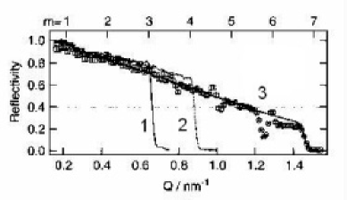
Figure 1: The measured neutron reflectivities of the Ni-Ti supermirrors fabricated with the large-scale ion-beam sputtering instrument (IBS) for the Spallation Neutron Source of J-PARC [1]. Reflectivities of 1) M3 mirror with 403 layers; 2) M4 mirror with 1201 layers; 3) M6.7 mirror with 8001 layers.

Last time all the mirrors were prepared in aperiodical fashion, which means that thicknesses of layers in bilayers vary with the bilayer number. F. Mezei and P.A. Dagleish performed the first experimental study of such supermirror in 1977 [2]. The algorithm for thickness variation was proposed by J.B. Hayter and H.A. Mook in 1989 [3]. According to this algorithm the change of thicknesses of neighboring bilayers is very small and does not match interatomic distance. It leads to creation of unavoidable roughnesses on layers interface. There exists also another algorithm proposed in [4], according to which the supermirror is to be produced as a set of periodic chains with some number N of identical bilayers. The variation of thicknesses of neighboring chains in this case is larger comparing to aperiodical systems, which may help to improve the quality of interfaces and therefore of the whole supermirror.

The goal of the given work is to investigate how well we can control the thickness and quality of periodic multilayer systems prepared by Mirrotron Ltd, Budapest. In other words we want to see how well the neutron reflectivity of produced systems match theoretical expectations, how large is diffuse scattering because of technological imperfectness and whether we can explain and control them.

Below we first present theoretical description of periodic multilayer systems, and calculate neutron reflectivities of periodic chains with N bilayers (N=2, 4, 8). Then we present results of measurements of reflectivities of fabricated multilayers and compare them to theoretical ones.

2 Theoretical description of periodical chains

A periodical chain consists of N bilayers every one of which contains two layers of different materials. In our case they were Ni and Ti. We call Ni with higher optical potential a “barrier”, and accept the real part of its potential $u_{b0}$, which is $2.45\cdot 10^{-7}$ eV, for unity. It means that the other energies are defined in units of $u_{b0}$. So, the full Ni potential with imaginary part is $u_{b}=1-0.00014i$. We call Ti with lower potential a “well”, and its optical potential in units of $u_{b0}$ is $u_{w}=-0.203-0.00012i$.

It was decided to investigate periodical stacks, that give Bragg reflection at the point $k=2$. This point is the normal to the sample surface component of the incident neutrons wave vector, and its value is given in units of the critical wave number $k_{c}=\sqrt{u_{b0}}$ of Ni. The point $k=2$ have to be at the center of the Darwin table of the Bragg peak. Our main task is to find thicknesses of the two sublayers of a bilayer, to get Bragg peak (at $N\to\infty$) with maximal width of the Darwin table.

Reflection amplitude of a periodical potential with N symmetrical periods is given by the equation [4]

$$R_{N}(k)=R_{\infty}\displaystyle\frac{1-\exp(2iqNa)}{1-R_{\infty}^{2}\exp(2iqNa)},$$ (1)

where

$$R_{\infty}=\frac{\sqrt{(1+r)^{2}-t^{2}}-\sqrt{(1-r)^{2}-t^{2}}}{\sqrt{(1+r)^{2}-t^{2}}+\sqrt{(1-r)^{2}-t^{2}}},$$ (2)

$$e^{iqa}=\frac{\sqrt{(1+t)^{2}-r^{2}}-\sqrt{(1-t)^{2}-r^{2}}}{\sqrt{(1+t)^{2}-r^{2}}+\sqrt{(1-t)^{2}-r^{2}}},$$ (3)

and $r$, $t$ are reflection and transmission amplitudes of a single period.

In the case of a bilayer the potential of a period is not symmetric, as is shown in Fig. 2.

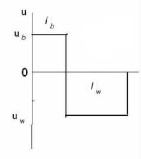
Figure 2: A single element of a multilayered system is a bilayer composed of two differen materials. The layer of one material has a high optical potential $u_{b}$ and a width $l_{b}$. The layer of the other material has lower potential $u_{w}$ and the width $l_{w}$.

Therefore we have to take into account a direction of reflection and transmission. We denote $\overrightarrow{r}$ the reflection amplitude for the incident wave propagating to the right, and $\overleftarrow{r}$ for the incident wave propagating to the left. Then

$$\overrightarrow{r}=r_{b}+t_{b}^{2}\displaystyle\frac{r_{w}}{1-r_{b}r_{w}},\qquad\overleftarrow{r}=r_{w}+t_{w}^{2}\displaystyle\frac{r_{b}}{1-r_{b}r_{w}},\qquad t=\displaystyle\frac{t_{b}t_{w}}{1-r_{b}r_{w}},$$ (4)

where

$$r_{b.w}=r_{0b,w}\displaystyle\frac{1-\exp(2ik_{b,w}l_{b,w})}{1-r_{0b,w}^{2}\exp(2ik_{b,w}l_{b,w})},\qquad t_{bw}=\exp(ik_{b,w}l_{b,w})\displaystyle\frac{1-r_{0b,w}^{2}}{1-r_{0b,w}^{2}\exp(2ik_{b,w}l_{b,w})},$$ (5)

$$r_{0b,w}=\displaystyle\frac{k-k_{b,w}}{k+k_{b,w}}\qquad k_{b,w}=\sqrt{k^{2}-u_{b,w}}.$$ (6)

We see that the transmission amplitude, $t$, is symmetric, i.e. it is the same in both directions. We can also introduce the symmetrized reflection amplitude

$$r=\sqrt{\overrightarrow{r}\overleftarrow{r}},$$ (7)

then, with account of asymmetry the equation (1) takes the form

$$\overrightarrow{R}_{N}(k)=\overrightarrow{R}_{\infty}\displaystyle\frac{1-\exp(2iqNa)}{1-R_{\infty}^{2}\exp(2iqNa)},$$ (8)

where $\overrightarrow{R}_{\infty}$ and $\overrightarrow{R}_{N}$ inherit the asymmetry of $r$, i.e.

$$\overrightarrow{R}_{\infty}=\displaystyle\frac{\overrightarrow{r}}{r}R_{\infty},\qquad\overrightarrow{R}_{N}=\displaystyle\frac{\overrightarrow{r}}{r}R_{N},$$ (9)

and $R_{N}$, $R_{\infty}$ are given by (1), (2) with symmetrized amplitude (7) used for $r$.

To find $l_{b,w}$ of the layers in the bilayer, which at $k=2$ give the center of the widest possible Darwin table with $|\overrightarrow{R}_{\infty}|=1$, we first neglect imaginary parts of the potentials $u_{b,w}$, and represent $t$ in the form $t=|t|\exp(i\psi)$ with real phase $\psi$. Then $r=\pm i|r|\exp(i\psi)$ with the same phase $\psi$, and Eq. (2) can be transformed to

$$R_{\infty}=\displaystyle\frac{\sqrt{\sin\psi(k)+|r(k)|}-\sqrt{\sin\psi(k)-|r(k)|}}{\sqrt{\sin\psi(k)+|r(k)|}+\sqrt{\sin\psi(k)-|r(k)|}}.$$ (10)

From it we see that the Bragg reflection takes place when $\sin^{2}\psi<|r|^{2}$, the center of the Darwin table is at $\sin\psi=0$ and the larger is $|r|$, the wider is the Darwin table. Therefore we must find the widths $l_{b,w}$ from two conditions:

$$\psi(l_{b},l_{w},k=2)=\pi,\qquad|r(2)|=\max(|r(l_{b},l_{w},k=2)|),$$ (11)

where we had shown dependence of $\psi$ and $|r|$ on widths $l_{b,w}$. To have the conditional maximum at the point $k=2$ we are to require maximum at this point of the function

$$F(l_{b},l_{w})=|r(l_{b},l_{w},k=2)|+\lambda[\psi(l_{b},l_{w},k=2)-\pi],$$ (12)

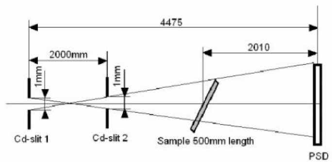
Figure 3: The scheme of the neutron reflectometer at KFKI. The sample mirror can be rotated around an axis perpendicular to the plane of the Fig. The position sensitive detector os stationary and sufficiently large to register all the reflected neutrons, when grazing angle is sufficiently small according to experimental requirements. Collimation angle was 0.5 mrad and the neutron beam was monochromatic with wave length 4.28 Å and presumable resolution ?

where $\lambda$ is the Lagrange multiplier. The maximum is found from three equations

$$\frac{d}{dl_{b}},\displaystyle\frac{d}{dl_{w}},\displaystyle\frac{d}{d\lambda}[|r|-\lambda(\psi-\pi)]=0.$$ (13)

Solution of these equations gives

$$k_{b}l_{b}=k_{w}l_{w}=\displaystyle\frac{\pi}{2}.$$ (14)

Therefore we must take

$$l_{b}=\displaystyle\frac{\pi}{2\sqrt{4-u_{b}}}=0.907,\qquad l_{w}=\displaystyle\frac{\pi}{2\sqrt{4-u_{w}}}=0.766.$$ (15)

The unit of length, corresponds to $k_{c}=1$ (Ni), therefore it is $\lambda_{c}/2\pi=92$ Å. So $l_{b}=83.4$ Å, and $l_{w}=70.4$ Å. It was decided to ask preparation of 3 samples with 2, 4 and 8 bilayers with thicknesses: Ni $l_{b}=84$ Å, and Ti $l_{w}=70$ Å.

3 Measurement and processing of data

In Figure 4 in linear scale are shown the results of fitting experimental data for 2, 4 and 8 periods with the formula:

$$R(k)=\int\limits_{k-\delta}^{k+\delta}|\overrightarrow{R}_{Ns}(p)|^{2}\displaystyle\frac{dp}{2\delta}+n_{b},$$ (16)

where

$$\overrightarrow{R}_{Ns}(p)=\overrightarrow{R}_{N}(p)+T^{2}_{N}(p)\displaystyle\frac{r_{s0}(p)}{1-\overleftarrow{R}_{N}(p)\,r_{s0}(p)}$$ (17)

is the reflection amplitude from a periodic chain of N periods evaporated over a semiinfinite substrate, and the substrate reflection amplitude is

$$r_{s0}=\displaystyle\frac{k-k_{s}}{k+k_{s}},\qquad k_{s}=\sqrt{k^{2}-u_{s}}.$$ (18)

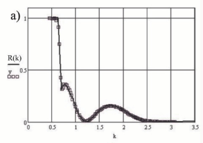
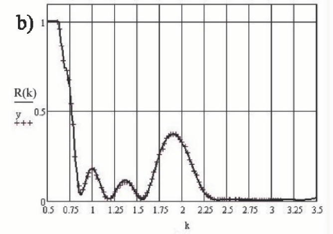
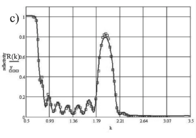
Figure 4: Fitting of the reflectivity data for periodic chains of bilayers evaporated on a thick float glass substrate. The fitting function is given by Equation (16). The data were obtained in Hungary at the reflectometer with wide stationary detector. The results are shown in linear scale for a) 2; b) 4; c)8 bilayers. The solid curves are theoretical curves with parameters found from fitting.

Eq. (16) takes into account the final resolution of the installation, scheme of which is shown in Fig. 3, and possible existence of background, $n_{b}$, in the system. The resolution $\delta$ and background $n_{b}$ were two fitting parameters. Besides them we took as fitting parameters the real parts of all the potentials $u_{b}$, $u_{w}$, the potential of substrate $u_{s}$ in terms of that of Ni, and thicknesses of Ni and Ti layers in units of $\lambda_{c}/2\pi$ of Ni. Imaginary parts of the potentials were calculated from absorption cross sections to be: $u^{\prime\prime}_{b}=0.00014$, $u^{\prime\prime}_{w}=0.00012$, and $u^{\prime\prime}_{s}=0.0001$. The last one was selected so small, because at first we thought that our substrate was pure silicon glass. The results for fitted parameters are presented in the first three lines of the Table 1. The last column of the table shows $\chi^{2}$ of the fitting.

N	$u^{\prime}_{b}$	$u^{\prime}_{w}$	$u^{\prime}_{s}$	$u^{\prime\prime}_{b}$	$u^{\prime\prime}_{w}$	$u^{\prime\prime}_{s}$	$l_{b}$	$l_{w}$	$\delta$	$n_{b}$	$\chi^{2}$
2	0.964	-0.258	0.452	0.00014	0.00012	0.0001	1.121	0.59	0.036	0.003	25
4	0.934	-0.388	0.446	0.00014	0.00012	0.0001	1.182	0.525	0.033	0.003	114
8	0.993	-0.242	0.398	0.00014	0.00012	0.0001	1.061	0.649	0.035	0.0089	349
8	0.963	-0.421	0.415	0.00014	0.00012	0.0001	1.169	0.54	0.036	0	209
8	0.972	-0.349	0.408	0.00014	0.00012	0.0001	1.13	0.579	0.036	0.003	151

Table 1: Fitted values of real parts of potentials $u^{\prime}$ for Ni (b-barrier), Ti (w-well) and substrate (s), their thickness $l$, resolution $\delta$, background $n_{b}$ and $\chi^{2}$ for periodic chains with N=2,4,8 bilayers. Imaginary parts $u^{\prime\prime}$ of the potentials were fixed. The results are given in dimensionless units. The unit of energy is equal to real part of Ni optical potential $u^{\prime}_{ni}=0.245\,\mu$eV, and unit of length is the reduced critical wavelength $\lambda_{c}/2\pi=92$ Å for Ni. The parameters at the 4-th line were obtained for zero background, and parameters of 5-th line were obtained for predetermined background $n_{b}=0.003$. It is interesting to see that the fitting with smaller number parameters (6 instead of 7) gave smaller $\chi^{2}$.

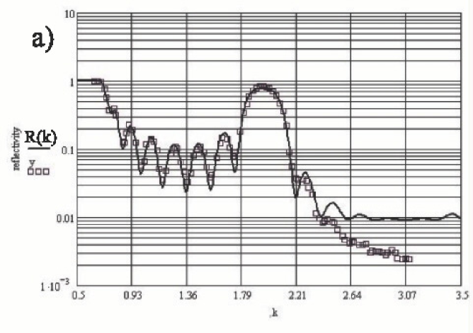
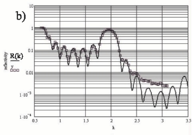
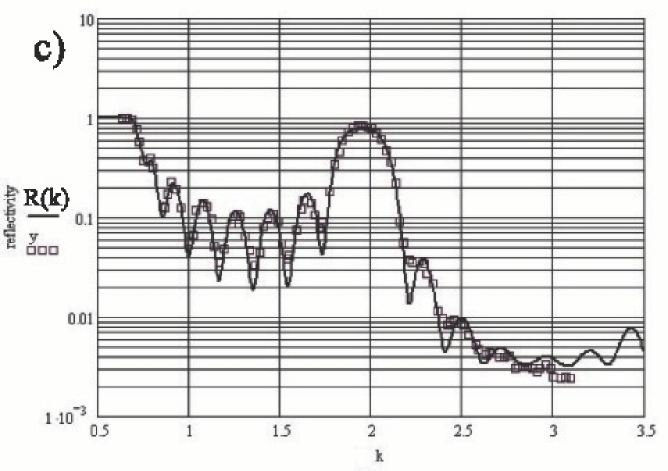
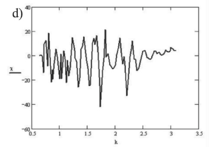
Figure 5: Logarithmic scale of different types of fitting of the reflectivity data from periodic chains of 8 bilayers on a thick float glass substrate. a) The fitting with 7 parameters, corresponding to Figure 4c); b) Fitting with 6 parameters ($n_{b}=0$); c) Fitting with 6 parameters ($n_{b}=0.003$); d) $\chi$-distribution in the case c).

The pictures in Fig. 4 show a good fit of all the samples, however the thicknesses of the Ni layers are more than 20% higher and thicknesses of the Ti layers are more than 20% lower than in the project. The Ni potential was found to be slightly lower than is expected, which can be explained by presence of some oxygen or nitrogen impurities. The substrate potential was found to be too high comparing to pure silicon glass, but later we found that it was boron glass the potential $u_{s}\approx 0.4$ for it is quite reasonable. The resolution $\delta\approx 3.5$ % and background $n_{b}=0.003$ are also quite acceptable. The worst was the value of the $\chi^{2}$. It is especially high in the case of the 8 periods sample.

The defects of fitting of the 8 periods sample are seen in Fig.  5 in logarithmic scale. In picture a), which corresponds to picture c) in Fig. 4, it is seen that theoretical line goes too high at large $k$. It corresponds to overestimated background $n_{b}=0.0089$. If we exclude $n_{b}$ from fitting parameters and put $n_{b}=0$ the other fitting parameters are changed as shown in 4-th line of the Table 1. The result of fitting in logarithmic scale is shown in picture b) of the Fig. 5. It is seen that the background in this case is underestimated. If we put background $n_{b}=0.003$ fixed at the same level as was obtained for samples with 2 and 4 periods, we obtain fitting parameters shown in 5-th line of the Table 1, and result of fitting in logarithmic scale shown in picture c) in Fig. 5. The parameter $\chi^{2}$ decreased (note that the number of fitting parameters in that case is 6, which is less than 7), however it is still too high, and in Fig. 5d) there is presented the $\chi$ distribution

$$\chi(k_{j})=\displaystyle\frac{R(k_{j})-y(k_{j})}{\sigma(k_{j})},$$ (19)

where $y(k_{j})$ and $\sigma(k_{j})$ are reflectivity and statistical error at experimentally measured points $k_{j})$. This distribution has very high fluctuations near minima of the data shown at picture c) and near the potential edge.

For analysis of the reason of so high fluctuations it was decided to analyze first the substrate.

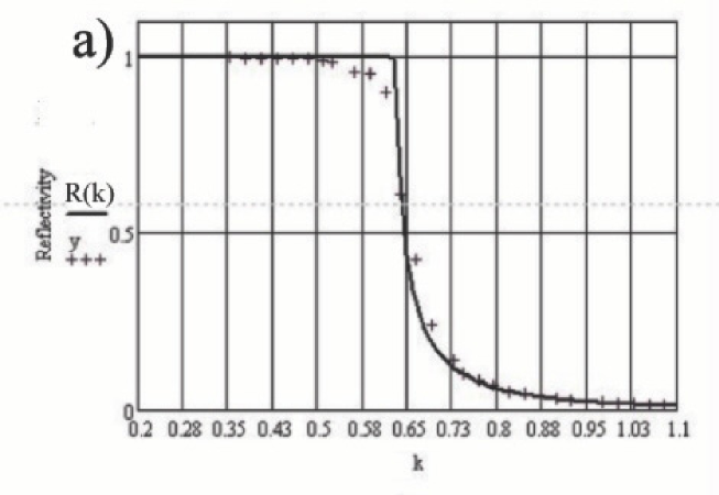
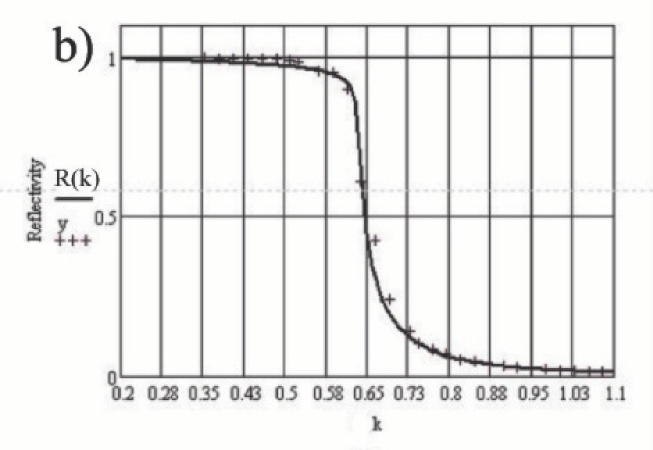
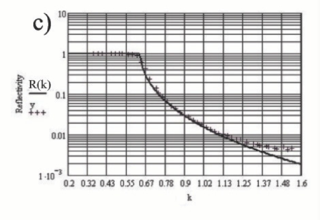
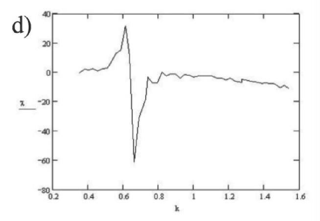
Figure 6: Fitting of the glass reflectivity data. a) One fitting parameter $u^{\prime}$; b) Two fitting parameters: $u^{\prime}$ and $u^{\prime\prime}$; c) Logarithmic scale of the Figure b); d) $\chi(k_{j})$ distribution for fitting with two parameters.

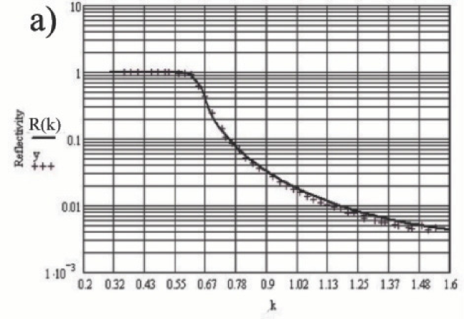
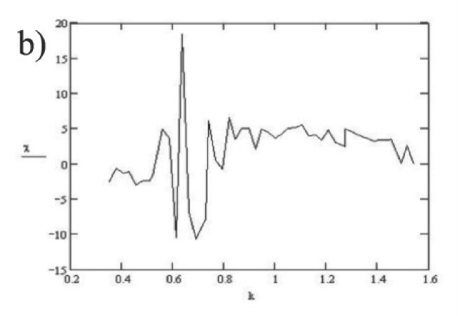
Figure 7: Fitting of the data for glass reflectivity a) with 4 parameters and $R(k)$ given by (21); b) Distribution of $\chi(k)$ for such fitting.

In Figure 6 there is presented the fitting of experimental data for substrate reflectivity fitted by function

$$R(k)=|r_{s0}(k)|^{2}$$ (20)

with one fitting parameter $u^{\prime}$, while $u^{\prime\prime}=0.0002$ was fixed. The result was $u^{\prime}=0.405$, which is in agreement with the fitting of periodic chains, and proves that the substrate is the boron glass, however $\chi^{2}=170$ was too high. In linear scale the graph is shown in Fig.  6a). The fitting with the same function but with 2 fitting parameters $u^{\prime}$ and $u^{\prime\prime}$ gives $u^{\prime}=0.406$ and $u^{\prime\prime}=0.00464$. In linear scale the graph is shown in Fig. 6b) and in logarithmic scale in Figure 6c). We see a strong deviation at large $k$. The parameter $\chi^{2}=137$ for such a fitting becomes a little bit less but remains still unacceptably high. The distribution $\chi(k)$ over all the experimental points is shown in Figure 6d).

In Fig.  7 are shown the result of fitting with more parameters. The picture a) shows fitting with 4 parameters according to Equation

$$R(k)=\int\limits_{k-\delta}^{k+\delta}|\overrightarrow{r}_{0}(p)|^{2}\displaystyle\frac{dp}{2\delta}+n_{b}.$$ (21)

The fitting parameters were $u^{\prime}$, $u^{\prime\prime}$, $\delta$ and $u_{b}$. It was obtained: $u^{\prime}=0.408$, $u^{\prime\prime}=0.003$, $\delta=4$% and $n_{b}=0.0024$, which is quite reasonable. The result of fitting in logarithmic scale is shown in Figure 7a).It looks quite well, however $\chi^{2}=31$, for this fitting is still too high. Distribution $\chi(k)$, shown in Figure 7b) demonstrates that there is still some peculiarity in experimental data near the critical edge.

4 Scattering at the interface

The anomaly near the potential edge of the substrate can appear because of scattering on surface roughness, on near surface inhomogeneities and even because of disordered distribution of atoms inside the glass [5]. The scattering at interface can be calculated with the help of distorted wave Born approximation (DWBA) i.e. with the help of Green function $G(u,k,\mbox{\boldmath$r$},\mbox{\boldmath$r$}^{\prime})$, which takes the interface into account.

4.1 Green function of DWBA

The Green function for reflection from the semiinfinite substrate satisfies the equation

$$\left(\Delta+k^{2}-\Theta(z>0)u\right)G(u,k,\mbox{\boldmath$r$},\mbox{\boldmath$r$}^{\prime})=-4\pi\delta(\mbox{\boldmath$r$}-\mbox{\boldmath$r$}^{\prime}),$$ (22)

where $u$ is the optical potential of an ideal medium at $z>0$. Since the space along the interface is uniform, the Green function can be represented by two dimensional Fourier integral

$$G(u,k,\mbox{\boldmath$r$},\mbox{\boldmath$r$}^{\prime})=-\int\frac{d^{2}p_{\|}}{\pi}\exp\left(i\mbox{\boldmath$p$}_{\|}(\mbox{\boldmath$r$}_{\|}-\mbox{\boldmath$r$}^{\prime}_{\|})\right)G(u,p_{\bot},z,z^{\prime}).$$ (23)

Substitution of it into Eq. (22) shows that $G(u,p_{\bot},z,z^{\prime})$ satisfies the equation

$$\left(d^{2}/dz^{2}+p^{2}_{\bot}-\Theta(z>0)u\right)G(u,p_{\bot},z,z^{\prime})=\delta(z-z^{\prime}).$$ (24)

According to common rules it can be constructed with the help of two linearly independent solutions $\psi_{1,2}(u,p_{\bot},z)$ of the homogeneous equation

$$\left(d^{2}/dz^{2}+p^{2}_{\bot}-\Theta(z>0)u\right)\psi_{1,2}(u,p_{\bot},z)=0.$$ (25)

For the function $\psi_{1}(u,p_{\bot},z)$ we can take

$$\psi_{1}(u,p_{\bot},z)=\Theta(z<0)\bigg{[}\exp(ik_{\bot}z)+r_{s0}(k_{\bot})\exp(-ik_{\bot}z)\bigg{]}+\Theta(z>0)t_{s0}(k_{\bot})\exp(ik^{\prime}_{\bot}z),$$ (26)

where $r_{s0}(x)$ is reflection amplitude (18), and $t_{s0}(x)=1+r_{s0}(x)$ is the refraction amplitude from vacuum into the substrate. For $\psi_{2}(u,p_{\bot},z)$ it is appropriate to take the function

$$\psi_{2}(u,p_{\bot},z)=\Theta(z<0)\exp(-ip_{\bot}z)t_{0s}(p_{\bot})+\Theta(z>0)\left(\exp(-ip^{\prime}_{\bot}z)-r_{s0}(p_{\bot})\exp(ip^{\prime}_{\bot}z)\right),$$ (27)

where $t_{0s}(x)=1-r_{s0}(x)$ is the refraction amplitude from substrate into the vacuum, and $p^{\prime}_{\bot}=\sqrt{p^{2}_{\bot}-u}$. The function (27) contains incident wave propagating inside the matter. The Wronskian of the functions $\psi_{1,2}(u,p_{\bot},z)$ is $w_{12}(p_{\bot})=2ip_{\bot}t_{0s}(p_{\bot})$.

With functions $\psi_{1}(u,p_{\bot},z)$ from (26) and $\psi_{2}(u,p_{\bot},z)$ from (27) we have

$$G(u,p_{\bot},z,z^{\prime})=\frac{\left(\Theta(z>z^{\prime})\psi_{1}(u,p_{\bot},z)\psi_{2}(u,p_{\bot},z^{\prime})+\Theta(z^{\prime}>z)\psi_{1}(u,p_{\bot},z^{\prime})\psi_{2}(u,p_{\bot},z)\right)}{2ip_{\bot}\tau^{\prime}(p_{\bot})}.$$ (28)

4.2 Scattering because of disorder

We first consider scattering because of disorder and incoherent scattering. Every atom $j$ inside the ordered medium composed of coherent scatterers is enlightened by the coherent wave field $\varphi(\mbox{\boldmath$r$}_{j})=t_{s0}(k_{\bot})\exp(i\mbox{\boldmath$k$}\mbox{\boldmath$r$}_{j})$ created by the incident wave $\exp(i\mbox{\boldmath$k$}\mbox{\boldmath$r$})$. However in presence of incoherency and disorder the enlightening field has fluctuations, which we denote $\delta\varphi(\mbox{\boldmath$r$}_{j})$, and suppose that their average $\overline{\delta\varphi(\mbox{\boldmath$r$}_{j})}=0$. These fluctuations produce scattered field

$$\delta\Psi(\mbox{\boldmath$r$})=\sum\limits_{j}G(u,k,\mbox{\boldmath$r$},\mbox{\boldmath$r$}_{j})\delta\varphi(\mbox{\boldmath$r$}_{j})b_{j}=\int d^{2}p_{\|}\exp(i\mbox{\boldmath$p$}\mbox{\boldmath$r$})A(\mbox{\boldmath$k$},\mbox{\boldmath$p$}),$$ (29)

where

$$A(\mbox{\boldmath$k$},\mbox{\boldmath$p$})=\frac{i\overrightarrow{t_{0}}(p_{\bot})}{2\pi p_{\bot}}\sum\limits_{j}\exp(-i\mbox{\boldmath$p$}^{\prime}\mbox{\boldmath$r$}_{j})\delta\varphi(\mbox{\boldmath$r$}_{j})b_{j},$$ (30)

the wave vector $p$ for the wave scattered into vacuum at $z<0$ is $\mbox{\boldmath$p$}=(\mbox{\boldmath$p$}_{\|},-p_{\bot})$, and $\mbox{\boldmath$p$}_{\bot}=\sqrt{k^{2}-p_{\|}^{2}}$. We can suggest that scattering amplitudes $b_{j}$ of $j$-th atom, and its fluctuating field are not correlated, therefore $\overline{\delta\varphi(\mbox{\boldmath$r$}_{j})b_{j}}=0$, and the correlation of this product for different atoms is described by the correlation function

$$\overline{\delta\varphi(\mbox{\boldmath$r$}_{j})b_{j}\delta\varphi(\mbox{\boldmath$r$}_{l})b_{l}|}=K\overline{|b|^{2}}|\varphi|^{2}(\mbox{\boldmath$r$}_{j})\{\delta_{jl}+g(|\mbox{\boldmath$r$}_{j}-\mbox{\boldmath$r$}_{l}|)\},$$

i.e. it is naturally supposed that correlation is proportional to $|\varphi|^{2}$ itself.

With the wave function (29) we can find the flux of scattered neutrons in the vacuum through any plane parallel to the substrate interface

$$J_{\bot}=\int\limits_{S}\frac{d^{2}r_{\|}}{2i}\left\langle\left[\overline{\delta}\Psi^{*}(\mbox{\boldmath$r$})\frac{d}{dz}\overline{\delta}\Psi(\mbox{\boldmath$r$})-\overline{\delta}\Psi(\mbox{\boldmath$r$})\frac{d}{dz}\overline{\delta}\Psi^{*}(\mbox{\boldmath$r$})\right]\right\rangle=(2\pi)^{2}\int\limits_{S}p_{\bot}\langle|A(\mbox{\boldmath$k$},\mbox{\boldmath$p$})|^{2}\rangle d^{2}p_{\|},$$ (31)

where $*$ means complex conjugate, and $S$ is some large area of the plane, over which we integrate. Ratio of this flux to the incident one $Sk_{\bot}$ gives scattering probability

$$w(\mbox{\boldmath$k$})=\frac{J_{\bot}(\mbox{\boldmath$k$})}{Sk_{\bot}}=\displaystyle\frac{(2\pi)^{2}}{S}\int\displaystyle\frac{p_{\bot}}{k_{\bot}}\langle|A(\mbox{\boldmath$k$},\mbox{\boldmath$p$})|^{2}\rangle d^{2}p_{\|}.$$ (32)

Since for scattered waves $\mbox{\boldmath$p$}^{2}=k^{2}$, and for propagating waves $p_{\bot}=\sqrt{k^{2}-p_{\|}^{2}}$ is a real number, then

$$d^{2}p_{\|}/p_{\bot}=2d^{3}p\delta(p^{2}-k^{2})=2\pi dp_{\bot},$$ (33)

and the last equality is correct when we can integrate over angle $d\phi$ around normal. As a result (32) is transformed to

$$w(\mbox{\boldmath$k$})=\displaystyle\frac{(2\pi)^{3}}{S}\int\limits_{0}^{k}\frac{p_{\bot}^{2}}{k_{\bot}}\overline{|A(\mbox{\boldmath$k$},\mbox{\boldmath$p$})|^{2}}dp_{\bot}.$$ (34)

With it we can define differential probability, or indicatrix

$$w(k_{\bot}\to p_{\bot})=(2\pi)^{3}\displaystyle\frac{p^{2}_{\bot}}{Sk_{\bot}}\overline{|A(\mbox{\boldmath$k$},\mbox{\boldmath$p$})|^{2}},$$ (35)

where

$$\overline{|A(\mbox{\boldmath$k$},\mbox{\boldmath$p$})|^{2}}=\left|\frac{t_{0s}(p_{\bot})}{2\pi p_{\bot}}\right|^{2}\overline{\sum\limits_{j,j^{\prime}}e^{-i\mbox{\boldmath$\kappa$}^{\prime*}\mbox{\boldmath$r$}_{j}}e^{i\mbox{\boldmath$\kappa$}^{\prime}\mbox{\boldmath$r$}_{j^{\prime}}}\delta\varphi(\mbox{\boldmath$r$}_{j})b_{j}\delta\varphi(\mbox{\boldmath$r$}_{j^{\prime}})b_{j^{\prime}}},$$ (36)

where $\mbox{\boldmath$\kappa$}^{\prime}=(\mbox{\boldmath$k$}_{\|}-\mbox{\boldmath$p$}_{\|},k^{\prime}_{\bot}+p^{\prime}_{\bot})$. The double sum has diagonal part, which after transformation to the integral over $N_{0}d^{3}r_{j}$ gives

$$\overline{|A(\mbox{\boldmath$k$},\mbox{\boldmath$p$})|^{2}}_{d}=\displaystyle\frac{N_{0}\overline{|b|^{2}}}{2(k^{\prime\prime}_{\bot}+p^{\prime\prime}_{\bot})}\left|\frac{t_{s0}(p_{\bot})t_{s0}(k_{\bot})}{2\pi p_{\bot}}\right|^{2}S,$$ (37)

and indicatrix

$$w_{d}(k_{\bot}\to p_{\bot})=N_{0}\overline{|b|^{2}}\displaystyle\frac{|t_{s0}(p_{\bot})t_{s0}(k_{\bot})|^{2}}{2k_{\bot}(k^{\prime\prime}_{\bot}+p^{\prime\prime}_{\bot})}.$$ (38)

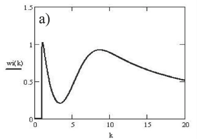
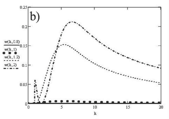
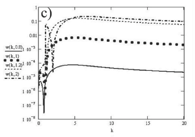
Figure 8: a) Function (44) in dependence on $k$ for $c=0.0001$, $u=1-i0.0002$, $a^{2}=0.2$, $b=5$; b) Function (43) in linear scale for several different $p$; c) the same as b) in logarithmic scale.

The nondiagonal part of the sum can be transformed to double integral:

$$\overline{\sum\limits_{j,j^{\prime}}F^{*}(\mbox{\boldmath$r$}_{j})F(\mbox{\boldmath$r$}_{j^{\prime}})}=N_{0}\int d^{3}r_{j}\int g(\mbox{\boldmath$r$}_{j}-\mbox{\boldmath$r$}_{j^{\prime}})F^{*}(\mbox{\boldmath$r$}_{j})F(\mbox{\boldmath$r$}_{j^{\prime}}),$$ (39)

where

$$g(\mbox{\boldmath$r$})=\delta(\mbox{\boldmath$r$})-N_{0}\gamma(\mbox{\boldmath$r$})$$ (40)

is correlation function chosen in such a way as to exclude the diagonal part of the sum. For simplicity we shall take for $\gamma(r)$ the Gaussian

$$\gamma(\mbox{\boldmath$r$})=(2\pi)^{-3/2}\exp(-r^{2}/2a^{2}),\quad a=N_{0}^{-1/3}.$$ (41)

After substitution of $\phi(\mbox{\boldmath$r$})$ into (36) and integration we obtain the expression

$$w_{nd}(\mbox{\boldmath$\Omega$}_{0}\to\mbox{\boldmath$\Omega$})=|b_{c}|^{2}N_{0}\frac{1}{k_{\bot}}|t_{s0}(p_{\bot})t_{s0}(k_{\bot})|^{2}\frac{1-\exp(-a^{2}\mbox{\boldmath$\kappa$}^{2}/2)}{p^{\prime\prime}_{\bot}+k^{\prime\prime}_{\bot}}\approx$$

$$\approx\frac{c}{k_{\bot}}|t_{s0}(p_{\bot})t_{s0}(k_{\bot})|^{2}\frac{1-\exp(-a^{2}[p^{\prime}_{\bot}-k^{\prime}_{\bot}]^{2}/2)}{p^{\prime\prime}_{\bot}+k^{\prime\prime}_{\bot}},$$ (42)

where in the last equality we put $c=|b_{c}|^{2}N_{0}$, and approximated $\kappa^{2}\approx[p^{\prime}_{\bot}-k^{\prime}_{\bot}]^{2}$, which is valid for small $p^{\prime}_{\bot}$ and $k^{\prime}_{\bot}$ and small angle between $k$ and $p$.

The function (42) represented in the form

$$w_{nd}(k,p)=\frac{c}{k}\frac{\left|t_{s0}(p)t_{s0}(k)\right|^{2}}{p^{\prime\prime}+k^{\prime\prime}}[1-\exp(-a^{2}[p^{\prime}-k^{\prime}]^{2}/2)],$$ (43)

and its integral,

$$wi(k)=c\int\limits_{0}^{b}\frac{dp}{k}\frac{\left|t_{s0}(p)t_{s0}(k)\right|^{2}}{p^{\prime\prime}+k^{\prime\prime}}[1-\exp(-a^{2}[p^{\prime}-k^{\prime}]^{2}/2)],$$ (44)

for $c=10^{-4}$, $a^{2}=0.2$, $b=5$ are shown in Figure 8. The curves are sensitive to parameter $a$ and the upper integration limit $b$. With increase of $b$ the left maximum in Figure 8a) increases comparing to the right one, and the right peak shifts to higher $k$.

4.3 Fitting of the experimental data for boron glass

The function (44) has two maxima, so we can hope to get better fitting for glass reflectivity shown in Figure 7a). In fitting we accepted potential of Boron glass to be $u=0.408-0.003i$ as was obtained above. We also included smoothing of the interface with Debye-Waller factor, i.e instead of $\overrightarrow{r_{0}}(k)$ we used $r_{m}(k)\equiv\overrightarrow{r_{0}}(k)\exp(-2h^{2}kk^{\prime})$, where $2h^{2}$ was a fitting parameter.

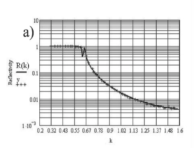
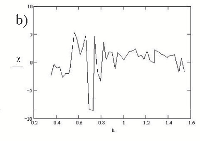
Figure 9: a) Result of fitting in logarithmic scale of reflectivity from boron glass with function (45). The glass potential $u=0.408-0.003i$ was fixed. The fitting parameters were found to be: $c=6.323\cdot 10^{-4}$, $a^{2}/2=0.102$, $\delta=0.022$, $n_{b}=2.401\cdot 10^{-3}$ and $h^{2}=0.048$. All the values are quite reasonable. b) $\chi$ distribution for such fitting. We see that some fluctuations still remain near the edge, but their amplitude decreased much comparing to that of Figure 7d).

Scattering on randomness and fluctuations was represented by function

$$w_{1}(k)=c\int\limits_{0}^{b}\frac{dp}{k}\frac{\left|t_{s0}(p)t_{s0}(k)\right|^{2}}{p^{\prime\prime}+k^{\prime\prime}}[2-\exp(-a^{2}[p^{\prime}-k^{\prime}]^{2}/2)].$$ (45)

The number 2 in brackets shows that we take the sum of two functions (42) and (38). In the function (45) there are two fitting parameters: factor $c$ and $a^{2}/2$.

The specular reflectivity was defined as $R_{s}(k)=|r_{m}(k)|^{2}-w_{1}(k)$, because scattering decreases specular reflectivity. For the total reflectivity we used the expression

$$R(k)=\int\limits_{k-\delta}^{k+\delta}R_{s}(k)\displaystyle\frac{dp}{2\delta}+n_{b}+w_{1}(k),$$ (46)

which contains two more fitting parameters: $\delta$ and $n_{b}$. Thus in total we had 5 fitting parameters. The result of fitting is shown in Figure 9. For upper limit of the integral $b=9$ in (45) the $\chi^{2}$ was 8.5. Though it is too high, it decreased considerably from value 31. The most important result is that fitting shows a dip in reflectivity near the edge. Fitting parameters were found to be: $c=8.3\cdot 10^{-4}$, which corresponds to randomness of positions of all the atoms in the glass; $a^{2}=0.204$, which means that correlation length is near 40 Å; resolution $\delta=2.2$%, which is better than in previous fittings; background $n_{b}=2.4\cdot 10^{-3}$ is nearly the same as before; and $2h^{2}=0.048$, i.e. $h\approx 15$Å, which means that in preparation of the float glass some Sn atoms diffused into the glass to the depth of 15Å. Results of fitting shows that the dip near the edge is quite well described by nonspecular reflectivity, and is not a result of some instrumental peculiarity. The dip in $\chi$ near the potential edge means that measured quantity is larger than theoretical one. It happens because in theory we does not take into account the neutrons scattered into the glass. These scattered neutrons after going through the sample can be registered by the detector. Because of them (the scattering is maximal near the edge due to Yoneda effect) experimental result is higher than theoretical one.

4.4 Scattering on roughnesses at the interface.

The usual approach is to consider roughness as a Gaussian process. It means that all the rough surface is treated as a single inhomogeneity and the scattered wave function is put down as

$$\Psi_{s}(\mbox{\boldmath$k$},\mbox{\boldmath$r$})=\int d^{2}p_{\|}\exp(i\mbox{\boldmath$p$}\mbox{\boldmath$r$})A(\mbox{\boldmath$k$},\mbox{\boldmath$p$}),$$ (47)

where

$$A(\mbox{\boldmath$k$},\mbox{\boldmath$p$})=-N_{0}b\frac{it_{0s}(p_{\bot})t_{0s}(k_{\bot})}{2\pi p_{\bot}}f(\mbox{\boldmath$\kappa$}^{\prime}).$$ (48)

Here

$$f(\mbox{\boldmath$\kappa$})=\int d^{2}r^{\prime}_{\|}\int\limits_{0}^{\zeta(\mbox{\boldmath$r$}^{\prime}_{\|})}dz^{\prime}\exp(i\mbox{\boldmath$\kappa$}\mbox{\boldmath$r$}^{\prime})=\int\displaystyle\frac{d^{2}r^{\prime}}{i\kappa_{\bot}}\exp(i\mbox{\boldmath$\kappa$}_{\|}\mbox{\boldmath$r$}^{\prime}_{\|})[\exp(i\kappa_{\bot}\zeta(\mbox{\boldmath$r$}^{\prime}_{\|}))-1]\Theta(\zeta(\mbox{\boldmath$r$}^{\prime}_{\|})>0),$$ (49)

if roughness is a cavity (note that its scattering density is $-N_{0}b$, and $\mbox{\boldmath$\kappa$}^{\prime}=(\mbox{\boldmath$\kappa$}_{\|},k^{\prime}_{\bot}+p^{\prime}_{\bot})$, where $q^{\prime}_{\bot}=\sqrt{q^{2}_{\bot}-u_{0}}$), and

$$A(\mbox{\boldmath$k$},\mbox{\boldmath$p$})=N_{0}b\int d^{2}r^{\prime}_{\|}\exp(i\mbox{\boldmath$\kappa$}_{\|}\mbox{\boldmath$r$}^{\prime}_{\|})\int\limits_{\zeta(\mbox{\boldmath$r$}^{\prime}_{\|})}^{0}dz^{\prime}\Theta(\zeta(\mbox{\boldmath$r$}^{\prime}_{\|})<0)\times$$

$$\times[\exp(ik_{\bot}z^{\prime})+r_{s0}(k_{\bot})\exp(-ik_{\bot}z^{\prime})][\exp(ip_{\bot}z^{\prime})+r_{s0}(p_{\bot})\exp(-ip_{\bot}z^{\prime})],$$ (50)

if roughness is a bump above the average interface. The parameter $\zeta$ is a random variable with probability density distribution

$$P(\zeta)=\displaystyle\frac{1}{\sigma\sqrt{2\pi}}\exp(-\zeta^{2}/2\sigma^{2}),$$ (51)

where $\sigma$ characterizes the average height of roughnesses. Averaging both of expressions over $\zeta$ we obtain corrections to specular reflectivity amplitude. It will be a combination of error function $\Phi(q\sigma)$, where $q=k_{\bot}\pm p_{\bot}$ or $q=k^{\prime}_{\bot}+p^{\prime}_{\bot}$.

For averaging of $|A(\mbox{\boldmath$k$},\mbox{\boldmath$p$})|^{2}$, which depends on random variables $\zeta$ at two different points $\mbox{\boldmath$r$}^{\prime}_{\|}$ we need the density distribution of the Gaussian process

$$P(\zeta_{1},\zeta_{2})=\displaystyle\frac{1}{2\pi\sigma^{2}\sqrt{1-K^{2}(\mbox{\boldmath$r$}_{\|})}}\exp\left(-\displaystyle\frac{\zeta_{1}^{2}+\zeta_{2}^{2}-2\zeta_{1}\zeta_{2}K(\mbox{\boldmath$r$}_{\|})}{2\sigma^{2}(1-K^{2}(\mbox{\boldmath$r$}_{\|}))}\right),$$ (52)

where $K$ is a correlation function, which depends on distance $r_{\|}$ between two points, where $\zeta_{1,2}$ are defined.

Small roughnesses

Though calculations with these formulas can be done up to the end without principal difficulties, we shall not proceed this complicated way and simplify our task assuming that the height, $\sigma$, of roughnesses is sufficiently small [6], i.e. $\sigma k_{\bot}\ll 1$. For small grazing angles it means that $\sigma\ll 100$ Å, which is quite practical. In that case we can accept $A(\mbox{\boldmath$k$},\mbox{\boldmath$p$})$ in the form

$$A(\mbox{\boldmath$k$},\mbox{\boldmath$p$})=-N_{0}b\frac{it_{0s}(p_{\bot})t_{0s}(k_{\bot})}{2\pi k_{\bot}}\int d^{2}r^{\prime}_{\|}\zeta(\mbox{\boldmath$r$}^{\prime}_{\|})\exp(i\mbox{\boldmath$\kappa$}\mbox{\boldmath$r$}^{\prime})$$ (53)

for all positive and negative $\zeta$. With this function we do not have corrections to $\overrightarrow{r_{0}}$, because $\langle\zeta\rangle=0$. The scattered waves are determined by

$$\int d^{2}r^{\prime}_{1\|}\exp(i\mbox{\boldmath$\kappa$}_{\|}\mbox{\boldmath$r$}^{\prime}_{1\|})\int d^{2}r^{\prime}_{2\|}\exp(i\mbox{\boldmath$\kappa$}_{\|}\mbox{\boldmath$r$}^{\prime}_{2\|})\zeta(\mbox{\boldmath$r$}^{\prime}_{1\|})\zeta(\mbox{\boldmath$r$}^{\prime}_{2\|}).$$ (54)

Averaging of $\zeta(\mbox{\boldmath$r$}^{\prime}_{1\|})\zeta(\mbox{\boldmath$r$}^{\prime}_{2\|})$ over (52) gives

$$\langle\zeta(\mbox{\boldmath$r$}^{\prime}_{1\|})\zeta(\mbox{\boldmath$r$}^{\prime}_{2\|})\rangle=\sigma^{2}K(\mbox{\boldmath$r$}^{\prime}_{1\|}-\mbox{\boldmath$r$}^{\prime}_{2\|}).$$ (55)

Therefore

$$\langle|A(\mbox{\boldmath$k$},\mbox{\boldmath$p$})|^{2}\rangle=S\displaystyle\frac{|N_{0}b\sigma|^{2}}{(2\pi p_{\bot})^{2}}\left|t_{0s}(p_{\bot})t_{0s}(k_{\bot})\right|^{2}\int d^{2}r^{\prime}_{\|}\exp(i\mbox{\boldmath$\kappa$}_{\|}\mbox{\boldmath$r$}^{\prime}_{\|})K(r^{\prime}_{\|}),$$ (56)

and indicatrix of nonspecular scattering is

$$w(k\to p)=2\pi\displaystyle\frac{|N_{0}b\sigma|^{2}}{k}\left|t_{0s}(p)t_{0s}(k_{\bot})\right|^{2}\int d^{2}r^{\prime}_{\|}\exp(i\mbox{\boldmath$\kappa$}_{\|}\mbox{\boldmath$r$}^{\prime}_{\|})K(r^{\prime}_{\|}).$$ (57)

To finish calculations we need to define correlation function. It is natural to suppose that

$$K(\mbox{\boldmath$r$}_{\|})=\exp(-r_{\|}^{2}/2l^{2}),$$ (58)

where $l$ is correlation length, or average dimension of roughnesses along the interface. With this function we have

$$K_{F}(\mbox{\boldmath$\kappa$}_{\|})=\int d^{2}r^{\prime}_{\|}\exp(i\mbox{\boldmath$\kappa$}_{\|}\mbox{\boldmath$r$}^{\prime}_{\|})\exp(-r_{\|}^{2}/2l^{2})=2\pi l^{2}\exp(-l^{2}\mbox{\boldmath$\kappa$}_{\|}^{2}/2),$$ (59)

and substitution into (57) gives

$$w(k\to p)=|N_{0}bl\sigma|^{2}\displaystyle\frac{(2\pi)^{2}}{k}\left|t_{0s}(p)t_{0s}(k_{\bot})\right|^{2}\exp(-l^{2}\mbox{\boldmath$\kappa$}_{\|}^{2}/2).$$ (60)

4.5 Scattering and fitting of periodic chains

There are a lot of opportunities how to include roughness at interfaces in multilayer systems. We can suppose that roughnesses are independent on every interface, or they can correlate between interfaces. It seems, that with sufficiently many fitting parameters it is possible to fit any result. However we shall not go this way. Because of so many opportunities it is better first to study experimentally the angular distribution of non specularly reflected neutrons, find its distinctive features and after that compare them with theoretical predictions based on different theoretical models. This is the way we are going proceed further.

5 Supermirror

Besides of the samples described above there was also prepared in BNC Budapest a supermirror M2, which consisted of 8 periodic chains and total number of 59 bilayers. The periods and number of them were found according to the above prescription with some corrections. The result of measurements comparing to calculations, in which we put Ni potential to be 0.964-0.005i and Ti potential -0.26-0.005i, is shown in Figure 10a). We see good coincidence. If we limit calculation of $\chi^{2}$ to the range $k<2$, then $\chi^{2}=7$, which is not bad, if to take into account that there were no fitting at all except some guess about imaginary parts of the potentials. The imaginary parts are higher than table ones because of possible impurities, inhomogeneities and surface roughness.

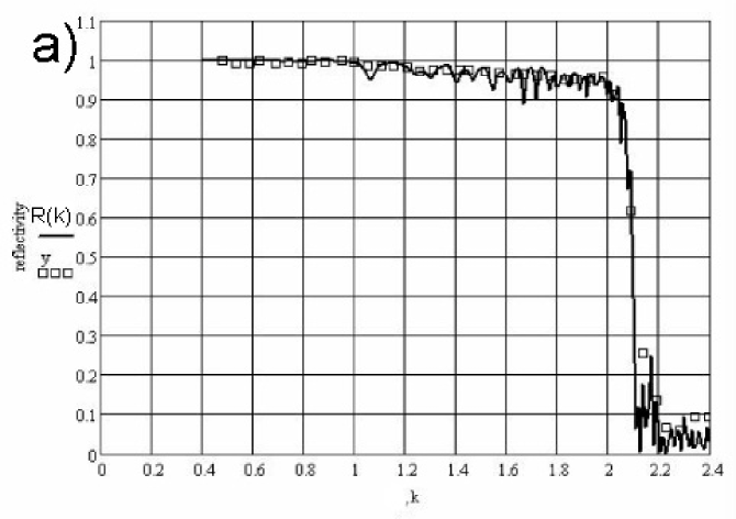
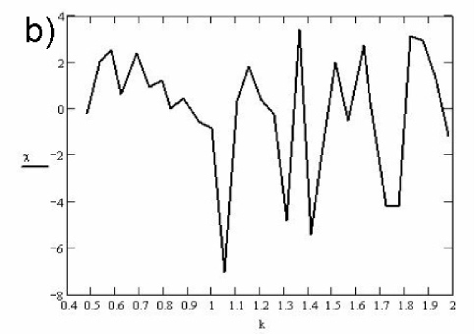
Figure 10: a)Experimental data points and theoretical calculation of supermirror M2.b) Distribution $\chi(k)$. It is obtained from direct comparison of experimental and theoretical date without fitting.

6 Conclusion

Cooperation of theoreticians and experimentalists in research of multilayer systems is found to be very fruitful. We see that technology of preparation of such systems by Mirrotron Ltd, Budapest is good, but it can be further improved after analysis of surface imperfection and their correlation with parameters of producing systems. This analysis can be performed with new experiments aimed at investigation of diffuse scattering and angular distribution of reflected neutron with better angular resolution.

References

- [1] Maruyama R, Yamazaki D, T. Ebisawa T, M. Hino M, Soyama K. Development of neutron supermirror with large critical angle. Thin solid films 2007;515:5704-6.
- [2] Mezei F, and Dagleish PA. Comm. Phys. 1977;2:41.
- [3] Hayter JB, Mook HA. Discrete Thin-Film Multilayer Design for X-ray and Neutron Supermirrors. J.Appl.Cryst. 1989;22:35-41.
- [4] Carron I., Ignatovich VK. Algorithm for preparation of multilayer systems with high critical angle of total reflection Phys.Rev. 2003;A67:043610.
- [5] Ignatovich VK. “Neutron optics.” M: Fizmatlit, 2006 (in Russian).
- [6] Steyerl A. Effect of surface roughness on the total reflection and transmission of slow neutrons. Z.Phys. 1972;254:169-88.
- [7] Sinha SK, Sirota EB, Garoff G, Stanley HB. X-ray and neutron scattering from rough surfaces. Phys.Rev.B 1988;38(4):2297-311.
- [8] Chiarello R, Panella V, Krim J, Thompson C. X-ray reflectivity and adsorption isotherm study of fractal scaling in vapor-deposited films. Phys.Rev.Lett. 1991;67(24):3408-11.
- [9] Pynn R. Neutron scattering by rough surfaces at grazing incidence. Phys.Rev.B. 1992;45(2):602-12.