Closed inflationary universe in Patch Cosmology

Abstract

In this article we study closed inflationary universe models using the Gauss-Bonnet Brane. We determine and characterize the existence of a universe with $\Omega>1$, with an appropriate period of inflation. We have found that this model is less restrictive in comparison with the standard approach where a scalar field is considered. We use recent astronomical observations to constrain the parameters appearing in the model.

I Introduction

Cosmological inflation has become an integral part of the standard model of the universe. Apart from being capable of removing the shortcomings of the standard cosmology, it gives important clues for structure formation in the universe. The scheme of inflation IC (see libro for a review) is based on the idea that at early times there was a phase in which the universe evolved through accelerated expansion in a short period of time at high energy scales. During this phase, the universe was dominated by a potential $V(\phi)$ of a scalar field $\phi$, which is called the inflaton.

Normally, inflation has been associated with a flat universe, due to its ability to effectively drive the spatial curvature to zero. In fact, requiring sufficient inflation to homogenize random initial conditions, drives the universe very close to its critical density. In this context, the recent observations are entirely consistent with a universe having a total energy density very close to its critical value and having an almost scale invariant power spectrum Peiris:2003ff ; WMAP3 . Most people interpret these values as corresponding to a flat universe. But, according to this results, we might take the alternative point of view of a marginally open op1 ; op or closed Linde:2003hc ; Joel ; Cl universe, which at early times in its evolution presents an inflationary period of expansion.

Nowadays there is considerable interest in inflationary models motivated by string/M-theory (for a review see Refs.1 ). In particular, much attention has been focused on the brane world scenario (BW), where our observable four-dimensional universe is modelled as a domain wall embedded in a higher-dimensional bulk space 2 .

BW cosmology offers a novel approach to our understanding of the evolution of the universe, the most spectacular consequence of this scenario is the modification of the Friedmann equation. These kind of models can be obtained from superstring theory witten ; witten2 . For a comprehensible review on BW cosmology, see Refs. lecturer ; lecturer2 ; lecturer3 . Specifical consequences of a chaotic inflationary universe scenario in a BW model were previously described maartens , where it was found that the slow-roll approximation is enhanced by the modification of the Friedmann equation.

On the other hand, when a stage closed to the Big-Bang is studied, quantum effects should be included in the bulk. In the high dimensional theory, high curvature correction terms should be added to the Einstein Hilbert action. One of the correction term to this action is the so called Gauss-Bonnet (GB) combination. The GB term arises naturally as the leading order of the $\alpha^{\prime}$ expansion of heterotic superstring theory, where, $\alpha^{\prime}$ is the inverse string tension. In fact, all versions of string theory (except Type II) in $10$ dimensions include this term. Therefore, it could be interesting to make study the effects of the Gauss-Bonnet term on inflationary braneworld models Meng:2003pn ; Lidsey:2003sj ; Calcagni:2004as ; Kim:2004gs ; Kim:2004jc ; Kim:2004hu ; Murray:2006fw .

When the five dimensional Einstein-GB equations are projected on to the brane, a complicated Hubble equation is obtained Ch ; Davis:2002gn ; Gravanis:2002wy . Interestingly enough, this modified Friedmann equation reduces to a very simple equation $H^{2}\sim\rho^{q}$ with $q=1,2,2/3$ corresponding to General Relativity (GR), Randall Sundrum (RS) and GB regimes respectively. This situation motivated the ”patch cosmology” as a useful approach to study braneworld scenarios Calcagni:2004bh . This scheme makes use of a nonstandard Friedmann equation of the form $H^{2}=\kappa_{q}\rho^{q}$. Despite all the shortcomings of this approximate treatment of extra-dimensional physics, it gives several important first-impact information.

The purpose of the present work is to study closed inflationary universe models in the spirit of Linde’s work Linde:2003hc , where the matter content is confined to a four dimensional brane which is embedded in a five dimensional bulk where a Gauss-Bonnet (GB) contribution is considered. We study these models using the approach of patch cosmology.

The paper is organized as follows. In Sect. II we briefly review the cosmological equations in the Gauss-Bonnet brane world and present the patch cosmological equations for this model. In Sect. III we determine the characteristics of a closed inflationary universe model with a constant scalar potential. Also, we get the value of the scalar field, when inflation begins and we obtain the probability of the creation of a close universe from nothing. In Sect. IV we consider a chaotic inflationary model. In Sect. V the cosmological perturbations are investigated. Finally, in Sect. VI, we summarize our results.

II Cosmological Equations in Gauss-Bonnet brane

We start with the five-dimensional bulk action for the Gauss-Bonnet braneworld:

$$S = \frac{1}{2\kappa_{5}^{2}}\int_{bulk}d^{5}x\sqrt{-g_{5}}\left\{R-2\Lambda_{5}+\alpha\left(R^{\mu\nu\lambda\rho}R_{{}^{\mu\nu\lambda\rho}}-4R^{\mu\nu}R_{\nu\mu}+R^{2}\right)\right\}$$ (1)

$$+\int_{brane}d^{4}x\sqrt{-g_{4}}\left(\mathcal{L}_{matter}-\sigma\right),$$

where $\Lambda_{5}=-3\mu^{2}\left(2-4\alpha\mu^{2}\right)$ is the cosmological constant in five dimensions, with the $AdS_{5}$ energy scale $\mu$, $\alpha$ is the GB coupling constant, $\kappa_{5}=8\pi/m_{5}$ is the five dimensional gravitational coupling constant and $\sigma$ is the brane tension. For a Friedmann-Robertson-Walker (FRW) metric, the exact Friedmann-like equation becomes Ch ; Davis:2002gn ; Gravanis:2002wy

$$2\mu\sqrt{1+\frac{H^{2}}{\mu^{2}}}\left(3-4\alpha\mu^{2}+8\alpha H^{2}\right)+\frac{k}{a^{2}}=\kappa_{5}^{2}\left(\rho+\sigma\right),$$ (2)

where $\rho$ represents the energy density of the matter sources on the brane, $a$ is the scale factor, and $k=0,+1,-1$ represents a flat, closed or open spatial section, respectively. The modified Friedmann equation (2) encodes all cosmological information. Despite the rather complicated form of Eq. (2), it is possible to make progress if we use the dimensionless variable $\chi$ Lidsey:2003sj ,

$$\kappa_{5}^{2}(\rho+\sigma)=\left[{{2(1-4\alpha\mu^{2})^{3}}\over{\alpha}}\right]^{1/2}\sinh\chi\,,$$ (3)

The Friedmann equation can be written as

$$H^{2}={1\over 4\alpha}\left[(1-4\alpha\mu^{2})\cosh\left({2\chi\over 3}\right)-1\right]\,,$$ (4)

where $\chi$ represents a dimensionless measure of the energy density. The modified Friedman equation (4), together with Eq. (3), ensures the existence of one characteristic Gauss-Bonnet energy scale,

$$m_{\alpha}=\left[{{2(1-4\alpha\mu^{2})^{3}}\over{\alpha}\kappa_{5}^{4}}\right]^{1/8}\,,$$ (5)

such that the GB high energy regime ($\chi\gg 1$) occurs if $\rho+\sigma\gg m_{\alpha}^{4}$. Expanding Eq. (4) in $\chi$ and using (3), we find in the full theory three regimes for the dynamical history of the brane universe,

$\bullet$  Gauss-Bonnet regime (5D),

$$\rho\gg m_{\alpha}^{4}~{}\Rightarrow~{}H^{2}\approx\left[{\kappa_{5}^{2}\over 16\alpha}\,\rho\right]^{2/3}\,,$$ (6)

$\bullet$   Randall-Sundrum regime (5D),

$$m_{\alpha}^{4}\gg\rho\gg\sigma\equiv m_{\sigma}^{4}~{}\Rightarrow~{}H^{2}\approx{\kappa_{4}^{2}\over 6\sigma}\,\rho^{2}\,,$$ (7)

$\bullet$   Einstein-Hilbert regime (4D),

$$\rho\ll\sigma~{}\Rightarrow~{}H^{2}\approx{\kappa_{4}^{2}\over 3}\,\rho\,.$$ (8)

Clearly Eqs. (6), (7) and (8) are much simpler than the full Eq (2) and in a practical case one of the three energy regimes will be assumed. Therefore, patch cosmology can be useful to describe the universe in a region of time and energy in which Calcagni:2004bh

$$H^{2}=\kappa_{q}\rho^{q}-\frac{1}{a^{2}},$$ (9)

where $H=\dot{a}/a$ is the Hubble parameter and $q$ is a patch parameter that describes a particular cosmological model under consideration. The choice $q=1$ corresponds to the standard General Relativity with $\kappa_{1}=8\pi/3m_{p}^{2}$, where $m_{p}$ is the four dimensional Planck mass. If we take $q=2$, we obtain the high energy limit of the brane world cosmology, in which $\kappa_{2}=4\pi/3\sigma m_{p}^{2}$. Finally, for $q=2/3$, we have the GB brane world cosmology, with $\kappa_{2/3}=G_{5}/16\zeta$, where $G_{5}$ is the $5D$ gravitational coupling constant and $\zeta=1/8g_{s}$ is the GB coupling ($g_{s}$ is the string energy scale). The parameter $q$, which describes the effective degrees of freedom from gravity, can take a value in a non-standard set because of the introduction of non-perturbative stringy effects.Just to mention some possibilities, these are the presence of a complicated geometrical framework with either compact and non-compact extra dimensions, multiple and/or folding branes configurations, and so on. For instance, in Ref.Kim:2004hu it was found that an appropriate region to a patch parameter $q$ is given by $1/2=q<\infty$. On the other hand, from Cardassian cosmology it is possible to obtain a Friedmann equation like (9) as a consequence of embedding our observable universe as a 3+1 dimensional brane in extra dimensions. In fact, in Ref.Chung:1999zs a modified FRW equation was obtained in our observable brane with $H^{2}\sim\rho^{n}$ for any $n$. This result was obtained using five-dimensional Einstein equations plus the Israel boundary conditions that related the energy-momentum on the brane to the derivatives of the metric in the bulk.

Brane world models are characterized by the feature that standard model matter is confined to a 1+3 dimensional brane while gravity propagates in the higher dimensional bulk. In general terms, we should include the situation in which matter could be transferred from the bulk to the brane or vice-versa. This circumstance could be realizable only if the bulk contains an appropriate form of matter, expressed by a high dimensional component of the energy-momentum tensor. However, in this paper we will assume that the matter fields are restricted to a lower dimensional hypersurface (brane) and that gravity exists throughout the space-time (brane and bulk) as a dynamical theory of geometry. Also, for 4D homogeneous and isotropic (FRW) cosmology, an extended version of Birkhoff s theorem tells us that if the bulk space-time is AdS, it implies that the effect of the Weyl tensor (known as dark radiation) does not appear in the modified Friedmann equation Bi . Certainly, it could be interesting to consider this effect, but its study will be postponed for the present. Thus, the energy conservation equation on the brane follows directly from the Gauss-Codazzi equations. For a perfect fluid matter source it is reduced to the familiar form,

$$\dot{\rho}+3H\left(\rho+P\right)=0,$$ (10)

where $\rho$ and $P$ represent the energy and pressure densities, respectively. The dot denotes derivative with respect to the cosmological time $t$.

We consider that the matter content of the universe is a homogeneous inflaton field $\phi(t)$ with potential $V(\phi)$. Then the energy density and pressure are given by

$$\rho=\frac{\dot{\phi}^{2}}{2}+V(\phi)=P+2V(\phi),$$ (11)

and the energy conservation equation (10) becomes

$$\ddot{\phi}+3\,H\,\dot{\phi}+V_{,\phi}(\phi)=0\,\,.$$ (12)

From the effective Friedmann equation (9) we can obtain the equation of motion for the scale factor,

$$\ddot{a}=a\kappa_{q}\rho^{q-1}\left[\rho\left(1-\frac{3}{2}q\right)-\frac{3}{2}\,q\,P\right],$$ (13)

and for convenience we will use units in which $c=\hbar=1$.

III Constant Potential in Gauss Bonnet Brane

Following the scheme of Ref. Linde:2003hc , we study a closed inflationary universe, where inflation is driven by a single scalar field confined to the brane. First let us consider a simple model with the step-like effective potential described by: $V(\phi)=0$ at $\phi<0$; $V(\phi)=V_{0}=Constant$ at $0<\phi<\phi_{0}$ and $V(\phi)$ extremely steep for $\phi>\phi_{0}$. We consider that the birth of the inflating closed universe can be created ”from nothing”, in a state where the scalar field takes the value $\phi_{in}\leq\phi_{0}$ at the point with $\dot{a}=0$, $\dot{\phi}=0$ and the potential energy density in this point is $V(\phi_{in})\gtrsim V_{0}$ . If the effective potential for $\phi<\phi_{0}$ grows very sharply, then the scalar field instantly falls down to the value $\phi_{0}$, with potential energy $V(\phi_{0})=V_{0}$, and its initial potential energy $V(\phi_{in})\equiv\,V_{in}$ becomes converted to the kinetic energy. Since this process happens instantly we can consider $\dot{a}=0$, so that the scalar field arrives to the plateau with a velocity given by

$$\dot{\phi}_{0}\,=\,-\sqrt{2\,(V_{in}-V_{0})}\,\,,$$ (14)

where $\dot{\phi}_{0}$ is the initial velocity of the field $\phi$, immediately after rolling down to the flat part of the potential.

Thus, in order to study inflation in this scenario, we need to solve Eqs. (9) and (12) in the interval $0<\phi\leq\phi_{0}$, with initial conditions $\dot{\phi}=\dot{\phi}_{0}$, $a=a_{0}$ and $\dot{a}=0$. These equations have different solutions, depending on the value of $\dot{\phi}_{0}$ and the patch under consideration. From Eqs. (9) and (14), we obtain

$$\frac{\ddot{a}}{a}=\kappa_{q}\,V_{in}^{q-1}\left[V_{in}\left(1-3\,q\right)+3\,q\,V_{0})\right]\,\,.$$ (15)

Then, we notice that there are three different scenarios, depending on the particular value of $V_{in}$. First, in the particular case when

$$\frac{V_{0}}{V_{in}}\,=\,\frac{3\;q-1}{3\;q},$$ (16)

we see that the initial acceleration of the scale factor is $\ddot{a}=0$. Since initially $\dot{a}=0$, then the universe remain static and the scalar field moves with constant speed given by Eq. (14).

In the second case we have

$$\frac{V_{0}}{V_{in}}\,<\,\frac{3\;q-1}{3\;q}.$$ (17)

In this case the universe start moving with negative acceleration ($\ddot{a}<0$) from the state $\dot{a}=0$. Therefore, in the scalar field equation the term proportional to $\dot{\phi}$ describe a negative dissipative term which makes the motion of the field $\phi$ even faster, so that $\ddot{a}$ becomes more negative. This universe rapidly collapses.

The third case corresponds to

$$\frac{V_{0}}{V_{in}}\,>\,\frac{3\;q-1}{3\;q}.$$ (18)

Here we have $\ddot{a}>0$ and the universe enters into an inflationary stage.

Now we proceed to make a simple analysis of the cosmological Eqs. (9) and (12) for cases where the condition (18) is satisfied. In the interval $0<\phi<\phi_{0}$ the inflaton field equation becomes

$$\ddot{\phi}+3\,\frac{\dot{a}}{a}\,\dot{\phi}=0\,\,,$$ (19)

whose first integral is

$$\dot{\phi}^{2}(t)=\dot{\phi_{0}}^{2}\,\left[\frac{a_{0}}{a(t)}\right]^{6}\,\,.$$ (20)

The behavior of the scalar field implies that the evolution of the universe rapidly falls into an exponential regimen (inflationary stage) where the scale factor becomes $a\sim\,e^{H\,t}$, and the Hubble parameter for the patch cosmology reads as follows

$$H=\sqrt{\kappa_{q}\,V_{0}^{q}}.$$ (21)

Once the universe enters in the inflationary stage, the scalar field moves by an amount $\Delta\phi_{inf}$ and then stops. From Eq. (20) we get

$$\Delta\phi_{inf}=\frac{\dot{\phi_{0}}}{3H}\approx-\frac{1}{3}\sqrt{\frac{1}{\kappa_{q}\,V_{0}^{q-1}}}.$$ (22)

Notice that, when $q=1$ ($\kappa_{q=1}=\kappa_{1}=8\pi/3$), we obtain $\Delta\phi_{inf}\approx-\sqrt{\frac{1}{24\pi}}$, which coincides with the result obtained in Ref. Linde:2003hc , and in the case $q=2$ ($\kappa_{q=2}=\kappa_{2}=4\pi/3\;\sigma$), we get $\Delta\phi_{inf}\approx-\sqrt{\frac{\sigma}{12\pi\;V_{0}}}$, result which coincides with the high energy limit of the model studied in Ref.Joel .

In order to study the model at early times (i.e. before inflation takes place), we write the equation of motion of the scale factor Eq. (9) in the following convenient form

$$\ddot{a}(t)=2\kappa_{1}\,V_{0}\,a(t)\,\beta(t)\,\,,$$ (23)

where, we have introduced a time-dependent dimensionless parameter $\beta(t)$, defined as follows

$$\beta(t)=\frac{1}{2}\,\frac{\kappa_{q}\;\rho^{q-1}}{\kappa_{1}\,V_{0}}\,\left[\rho(1-\frac{3}{2}\,q)-\frac{3}{2}\,q\,p\right].$$ (24)

Now we proceed to make a simple analysis of the evolution of the scalar field and scale factor before inflation. With this purpose we consider initial conditions which satisfy $\beta(0)\equiv\beta_{0}\ll 1$. We can write

$$\beta_{0}=V_{in}^{q-1}\,[V_{in}-V_{*}]\,\frac{(1-3q)\,\kappa_{q}}{2\,V_{0}\,\kappa_{1}},$$ (25)

where we have defined $V_{*}=3qV_{0}/(3q-1)$.

Then, at the beginning of the process, we have $a(t)\approx a_{0}$ and $\beta(t)\approx\beta_{0}$, and Eq.(23) takes the form:

$$\ddot{a}(t)=2\kappa_{1}\,a_{0}V_{0}\beta_{0}\,\,.$$ (26)

For small $t$, the solution of this equation is

$$a(t)=a_{0}\left(1+\kappa_{1}\beta_{0}V_{0}t^{2}\right).$$ (27)

From Eqs. (20) and (27) we find that the time interval $\Delta t_{1}$ where $\beta(t)$ becomes twice as large as $\beta_{0}$ is given by

$$\Delta t_{1}\approx\sqrt{\frac{\kappa_{1}}{\kappa_{q}}}\;\left[4\pi\left(\frac{3}{2}\right)^{q-1}\,[(3q-1)+(q-1)^{2}]\;V_{0}^{q}\right]^{-1/2}.$$ (28)

This result is in agreement with Refs. Linde:2003hc ; Joel for the cases $q=1$ and $q=2$, ($\kappa_{1}/\kappa_{2}=2\sigma$) respectively.

Consequently, the scalar field decreases by the amount

$$\Delta\phi_{1}\sim\dot{\phi_{0}}\,\Delta t_{1}\approx-\sqrt{\frac{\kappa_{1}}{\kappa_{q}}}\;\left[2\pi\left(\frac{3}{2}\right)^{q-1}\,(3q-1)\;[(3q-1)+(q-1)^{2}]\;V_{0}^{q-1}\right]^{-1/2}.$$ (29)

We note that for a given $q$, this result depends on the value of $V_{0}$, and the decrease of the scalar field is less restrictive than the one used in the standard case $q=1$ in which $\Delta\phi_{1}=const.\sim-1/(2\sqrt{3\pi})$ Linde:2003hc . After the time $\Delta t_{2}\approx\Delta t_{1}$, the scalar field decreases by the amount $\Delta\phi_{2}\approx\Delta\phi_{1}$, and the rate of growth of $a(t)$ increases again. This process finishes when $\beta(t)\rightarrow\beta_{f}$, where $\beta_{f}=\kappa_{q}\,V_{0}^{q-1}/(2\kappa_{1})$.

Since at each interval $\Delta t_{i}$ the value of $\beta$ doubles, the number of intervals $n_{int}$ after which $\beta(t)\rightarrow\beta_{f}$ is

$$n_{int}=\frac{\ln\beta_{f}-\ln\beta_{0}}{\ln 2}\,\,.$$ (30)

Therefore, if we know the initial value of the scalar field, we can estimate the value of the scalar field at which inflation begins $\phi_{inf}$

$$\phi_{inf}\approx\phi_{0}-\left(\frac{\ln\beta_{f}-\ln\beta_{0}}{\ln 2}\right)\!\sqrt{\frac{\kappa_{1}}{\kappa_{q}}}\;\left[2\pi\left(\frac{3}{2}\right)^{q-1}\,(3q-1)\;[(3q-1)+(q-1)^{2}]\;V_{0}^{q-1}\right]^{-1/2}.$$ (31)

This expression indicates that our result for $\phi_{inf}$ is sensitive to the choice of the potential energy $V_{0}$, the patch parameter $q$, and the initial velocity of the scalar field $\phi$ immediately after it rolls down to the plateau of the potential energy.

Note that if the scalar field starts its motion with a small velocity, inflation begins immediately. On the other hand, if the field $\phi$ moves with a large initial velocity, inflation is delayed. After inflation, the field $\phi$ stops moving when it passes the distance $|\Delta\phi_{\inf}|$ (see Eq. (22)). Note that if the field stops before it reaches $\phi=0$, the universe expands forever in an inflationary stage. The same problem occurs in Einstein’s General Relativity model Linde:2003hc . However, in the context of patch cosmology ($q\neq 1$) the value of $\Delta\phi_{\inf}$ depends on the value we assign to the patch parameter and the other constants involved. Therefore, we will see that the problem of the universe inflating forever disappears and thus the inflaton field can reach the value $\phi=0$ for some appropriate conditions of the constants involved in our models.

Since inflation could occur only in the interval $\phi_{inf}>0$ and $\phi=0$, the initial value of the inflaton field satisfies

$$\phi_{0}>\left(\frac{\ln\beta_{f}-\ln\beta_{0}}{\ln 2}\right)\!\sqrt{\frac{\kappa_{1}}{\kappa_{q}}}\;\left[2\pi\left(\frac{3}{2}\right)^{q-1}\,(3q-1)\;[(3q-1)+(q-1)^{2}]\;V_{0}^{q-1}\right]^{-1/2}.$$ (32)

On the other hand, in order to determine the initial value of the scalar field $\phi_{0}$, we need to find the value of $\beta_{0}$. To perform this task, we study the birth of a closed universe in the patch cosmology. From the semiclassical point of view, the probability of creation of a closed universe from nothing is given by Koya

$$P\sim e^{-2\mid S_{E}\mid}=\exp\left(-\left[\frac{8\,\pi^{2}}{3\,\kappa_{q}^{2}}\right]\,\rho^{-(2q-1)}\right)\simeq\,\exp\left(-\left[\frac{8\,\pi^{2}}{3\,\kappa_{q}^{2}}\right]\,V^{-(2q-1)}\right),$$ (33)

where we have used Eq.(11) with $\dot{\phi}^{2}\ll V(\phi)$.

We estimate the conditional probability in order to create the universe with an energy density equal to $V_{in}$. We assume that this energy is smaller than $V_{*}$ so that it satisfies the condition expressed by Eq.(18). We get

$$P\sim e^{-2\mid S_{E}\mid}=\exp\left(-\left[\frac{8\,\pi^{2}}{3\,\kappa_{q}^{2}}\right]\,\left[\frac{1}{V_{in}^{2q-1}}-\frac{1}{V_{*}^{2q-1}}\right]\right)\,\,.$$ (34)

This expression tells us that the probability of creation of the universe with $\beta_{0}\neq 0$ is not exponentially suppressed if $\beta_{0}<\frac{6V_{0}}{m_{p}^{4}}$, $\beta_{0}<\frac{432}{625}\frac{V_{0}^{4}}{\sigma^{3}\,m_{p}^{4}}$, and $\beta_{0}<\frac{27\,m_{p}^{2}}{64\,\pi^{2}}\,\kappa_{2/3}^{3}$ for $q=1$, $q=2$ and $q=2/3$, respectively. See table (1). These conditions, together with Eq. (32), impose a bound from below for the initial value of the scalar field $\phi_{0}$.

Table 1: Probabilities of each patch cosmology and the initial value of the inflaton field $\phi_{0}$.

$q$	Probability	$\,\phi_{0}/m_{p}>$
$1$	$P\sim\exp\left(-\frac{\beta_{0}m_{p}^{4}}{6V_{0}}\right)$	$6.57$
$2$	$P\sim\exp\left(-\frac{625}{432}\frac{\sigma^{3}\beta_{0}m_{p}^{4}}{V_{0}^{4}}\right)$	11.10
$2/3$	$P\sim\exp\left(-\frac{64\pi^{2}}{27\,m_{p}^{2}}\frac{\beta_{0}}{k_{2/3}^{3}}\right)$	17.73

As an example, we take a particular set of the parameters appearing in our model. We consider $V_{0}\sim 10^{-11}m_{p}^{4}$ libro , $\kappa_{1}=8\pi/3m_{p}^{2}$ , $\kappa_{2}=4\pi/3\sigma\,m_{p}^{2}$ where the brane tension was taken as $\sigma=10^{-10}m_{p}^{4}$ and $\kappa_{2/3}=10^{-3}/m_{p}^{2/3}$. These values allow us to fix the initial condition of the inflaton field for the different patches. Table 1 shows our results.

Numerical solutions of the inflaton field $\phi(t)$ are shown in Fig. 1, where we have considered different values of the patch parameter. Note that the interval from $\phi_{0}$ to $\phi_{\inf}$ increases when the patch parameter $q$ increases, but its shape remain practically unchanged.

We can notice that for these three values of $q$, inflation begins immediately if the field $\phi$ starts its motion with sufficiently small velocity, in analogy with Einstein’s GR theory ($q=1$). On the other hand if it starts with large initial velocity the universe could does not present the inflationary period at any stage.

It is also worth mentioning, that in all patch cosmologies under study the inflaton field does not show oscillations,since in this case the scalar potential is a constant.

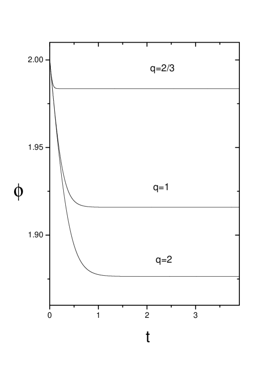
Figure 1: We plot the inflaton field $\phi$(t) as a function of the cosmological time by using the model $V=V_{0}=const.$ in the patch cosmology model. In all of them, we have taken the same value of $\dot{\phi_{0}}$. Here, we have used unit where $m_{p}=1$.

IV Chaotic potential

We consider an effective potential given by $V(\phi)=\lambda_{n}\,\phi^{n}$ for $\phi<\phi_{0}$, which becomes extremely steep for $\phi>\phi_{0}$. In particular, we take $\lambda_{n}$ as a free parameter, which in the special case $n=2$ is related to the mass of the scalar field Fairbairn:2002yp . In the following we will consider $\lambda_{n}>0$ and the cases $n=2,4$.

We assume that the whole process is divided in three parts. The first one corresponds to the creation of the closed universe “from nothing” in a state where the inflaton field takes the value $\phi_{in}\geq\phi_{0}$ at the point with $\dot{a}=0$, $\dot{\phi}=0$, and where the potential energy is $V_{in}$. If the effective potential for $\phi\ >\phi_{0}$ grows very sharply, then the scalar field instantly falls down to the value $\phi_{0}$, with potential energy $V(\phi_{0})$. Therefore, the initial potential energy becomes converted to kinetic energy, (see the previous section). Then, we have

$$\dot{\phi}^{2}_{0}=2(V_{in}-V(\phi_{0})).$$ (35)

Following the discussion of the previous section we assume that the following initial condition is satisfied:

$$V_{in}<\frac{3q}{(3q-1)}\,V(\phi_{0})\,,$$ (36)

which guarantees that the model arrives to an inflationary regimen. As it was mentioned previously, in all other cases the universe remains either static, or it collapses rapidly.

The following steps are described by Eqs. (9) and (12) in the interval $\phi\leq\phi_{0}$ with initial conditions $\dot{\phi}=\dot{\phi}_{0}$, $a=a_{0}$ and $\dot{a}=0$. In particular, the second part of the process corresponds to the motion of the inflaton field before the beginning of the inflation stage, and it is well described by the following approximated field equations.

$$\ddot{\phi}=-3\,\frac{\dot{a}}{a}\,\dot{\phi}\,,\\$$ (37)

and

$$\ddot{a}=2\kappa_{q}\,a\,V(\phi)\,\beta(t),$$ (38)

with $\beta(t)$ satisfying $\beta(t)\ll 1$, as in the previous section.

The last step corresponds to the stage of inflation where $\dot{\phi}$ is small enough and the scale factor $a(t)$ grows exponentially. This part is well described by the following equations

$$3\,\frac{\dot{a}}{a}\,\dot{\phi}=-V_{,\,\phi}\,\,,$$ (39)

$$\ddot{a}=\kappa_{q}\,a\,V(\phi)^{q}\,.$$ (40)

Now we will describe the process in more details. Let us consider the second stage, where the scalar field and the scale factor $a(t)$ satisfy Eqs.(37) and (38). Following the previous scheme, we solve the equation for $a(t)$ by considering $\beta(t)\ll 1$. Then, at the beginning of the process, when $a\approx a_{0}$ and $\beta\approx\beta_{0}$, Eq. (38) takes the form

$$\ddot{a}(t)=2\kappa_{1}\,a_{0}V(\phi_{0})\beta_{0}\,\,,$$ (41)

and the scalar field satisfies Eq.(20). The amount of the decreasing of the scalar field during the time $\Delta t$, which make the value of $\beta$ two times grater than $\beta_{0}$ is

$$\Delta\phi\approx-\sqrt{\frac{\kappa_{1}}{\kappa_{q}}}\;\left[2\pi\left(\frac{3}{2}\right)^{q-1}\,(3q-1)\;[(3q-1)+(q-1)^{2}]\;V(\phi_{0})^{q-1}\right]^{-1/2}.$$ (42)

This process continues until $\dot{\phi}$ becomes small enough, so that the universe begins to expand in an exponential way, characterizing the inflationary era. We take that the inflation begins when $\beta(t)$ tends to $\beta_{f}$, where $\beta_{f}=\kappa_{q}\,V(\phi_{0})^{q-1}/(2\kappa_{1})$. Then, according to our previous result, the field $\phi$ gets the value:

$$\phi_{inf}\approx\phi_{0}-\left(\frac{\ln\beta_{f}-\ln\beta_{0}}{\ln 2}\right)\!\sqrt{\frac{\kappa_{1}}{\kappa_{q}}}\;\left[2\pi\left(\frac{3}{2}\right)^{q-1}\,(3q-1)\;[(3q-1)+(q-1)^{2}]\;V(\phi_{0})^{q-1}\right]^{-1/2}.$$ (43)

During inflation the number of e-folds for our potential is given by

$$N\simeq\frac{3\kappa_{q}\,\lambda_{n}^{q-1}}{n(n(q-1)+2)}\,\phi^{n(q-1)+2}_{inf}\,.$$ (44)

We assume conclusively that for $N=60$ one would have $\Omega=1.1$. Then one can show that for $N=59.5$ and the same value of the Hubble constant one would get $\Omega\approx 1.3$, whereas for $N=60.5$ we obtain $\Omega\approx 1.03$ Linde:2003hc ; Cl . Notice that, in analogy with Einstein s theory of GR a fine tuning of the value of $V(\phi_{0})$ is required for having the value of $\Omega$ in the range $1\lesssim\Omega<1.1$.

One of the main prediction of any inflationary universe model is the primordial spectrum that arises due to quantum fluctuation of the inflaton field. Therefore, it is interesting to study the density perturbation behavior for our cosmology.

V Perturbations

Even though the study of scalar density perturbations in closed universes is quite complicated, it is interesting to give an estimation of the standard quantum scalar field fluctuations in this scenario. In particular, the amplitude of scalar perturbations generated during inflation for a flat space is Kim:2004gs

$$\delta_{H}^{2}=\frac{1}{25\pi^{2}}\,\frac{H^{2}}{\dot{\phi}^{2}}=\frac{1}{25\pi^{2}}\,\frac{9\kappa_{q}^{3}\,V^{3q}}{(V_{,\,\phi})^{2}}\,.$$ (45)

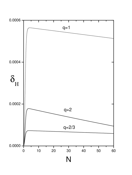
Figure 2: Scalar density perturbation as a function of the N e-folds. The plot shows the case $n=2$, for the potential $V(\phi)$. We have taken $\sigma=10^{-10}$, $\kappa_{2/3}=10^{-3}$ and we have used unit where $m_{p}=1$.

The slow-roll parameters are given by

$$\epsilon_{1}=-\frac{\dot{H}}{H^{2}} \simeq \frac{q\,(V_{,\,\phi})^{2}}{6\kappa_{q}\,V^{1+q}}\,,$$ (46)

$$\epsilon_{2}=-\frac{\ddot{H}}{H\,\dot{H}} \simeq \frac{1}{3\kappa_{q}}\,\left[\frac{q}{2}\,\frac{(V_{,\,\phi})^{2}}{V^{1+q}}-\frac{V_{,\,\phi\phi}}{V^{q}}\right].$$ (47)

Certainly, in our case, Eq.(45) is an approximation and must be supplemented by several different contributions in the context of a closed inflationary universe Linde:2003hc . However, one may expect that the flat-space expression gives a correct result for $N>3$.

If one interprets perturbations produced immediately after the creation of a closed universe (at $N\sim O(1)$) as perturbations on the horizon scale $l\sim 10^{28}cm$, then the maximum at $N\sim 10$ would correspond to the scale $l\sim 10^{24}cm$, and the maximum at $N\sim 15$ would correspond to the scale $l\sim 10^{22}cm$, which is similar to the galaxy scale.

We also consider the spectral index $n_{s}$, which is related to the power spectrum of density perturbations $\delta_{H}(k)$. For modes with a wavelength much larger than the horizon ($k\ll aH$), the spectral index $n_{s}$ is an exact power law, expressed by $\delta_{H}(k)\propto k^{n_{s}-1}$, where $k$ is the comoving wave number. The scalar spectral index is given by Kim:2004gs

$$n_{s}=1-4\epsilon_{1}-2\epsilon_{2}.$$ (48)

Following Ref.Kim:2004gs the running of the scalar spectral index for our model becomes

$$\alpha_{s}=\frac{dn_{s}}{d\ln k}\simeq\;-8\frac{\epsilon_{1}^{2}}{q}-10\epsilon_{1}\,\epsilon_{2}+2\epsilon_{2}^{2}-2\epsilon_{3},$$ (49)

where we have used that $d\ln k=-dN$ and $\epsilon_{3}$ is given by

$$\epsilon_{3}\simeq\frac{1}{9\kappa_{q}^{2}}\,\left[\frac{V_{,\,\phi}\,V_{,\,\phi\phi\phi}}{V^{2q}}+\frac{(V_{,\,\phi})^{2}}{V^{2q}}-\frac{5q}{2}\frac{(V_{,\,\phi})^{2}V_{,\,\phi\phi}}{V^{2q+1}}+\frac{q(q+2)}{2}\frac{(V_{,\,\phi})^{4}}{V^{2(q+1)}}\right].$$

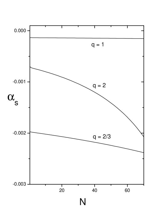
Figure 3: This plot shows the running spectral index, $\alpha_{s}$, as a function of the N e-folds, for the case $n=2$. We have taken $\sigma=10^{-10}$, $\kappa_{2/3}=10^{-3}$ and used $m_{p}=1$.

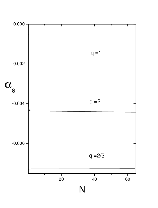
Figure 4: Plot shows the running spectral index as a function of the N e-folds, for the case $n=4$. We have taken $\sigma=10^{-10}$, $\kappa_{2/3}=10^{-3}$ and using $m_{p}=1$.

In models with only scalar fluctuations, the marginalized derivative value of the spectral index is approximated by $dn_{s}/d\ln k=\alpha_{s}\sim-0.03$ for Wilkinson Microwave Anisotropy Probe (WMAP) five-year data only WMAP3 .

Actually, with this data, together with Sloan Digital Sky Survey (SDSS) large scale structure surveys Teg , an upper bound for $\alpha_{s}(k_{0}$) was found, where $k_{0}$=0.002 Mpc^-1 corresponds to $L=\tau_{0}k_{0}\simeq 30$, with the distance to the decoupling surface $\tau_{0}$= 14,400 Mpc. SDSS measures galaxy distributions at red-shifts $a\sim 0.1$ and probes $k$ in the range 0.016 $h$ Mpc^-1$<k<$0.011 $h$ Mpc^-1. The recent WMAP five-year data results give the value for the scalar curvature spectrum $P_{\cal R}(k_{0})\equiv\,25\delta_{H}^{2}(k_{0})/4\simeq 2.4\times\,10^{-9}$ . This value allows us to find constraints on the parameters appearing in our model. In particular, for $N=10$, we have $\delta_{H}\approx 5.6\times 10^{-4}$ for $q=1$, $\delta_{H}\approx 1.6\times 10^{-4}$ for $q=2$, and $\delta_{H}\approx 7.2\times 10^{-5}$ for $q=2/3$. In the particular case when $n=2$, the running of the scalar spectral index $dn_{s}/d\ln k=\alpha_{s}$ are given by $\alpha_{s}\sim-1.4\times 10^{-4}$ for $q=1$, $\alpha_{s}\sim-8.0\times 10^{-4}$ for $q=2$, and $\alpha_{s}\sim-0.002$ for $q=2/3$. For $n=4$, it is found $\alpha_{s}\sim-5.4\times 10^{-4}$ for $q=1$, $\alpha_{s}\sim-0.004$ for $q=2$, and $\alpha_{s}\sim-0.007$ for $q=2/3$.

VI Conclusion and Final Remarks

In this work we have studied a closed inflationary universe model in which the gravitational effects are described by the Gauss-Bonnet Brane World Cosmology. We study this model by using the scheme of patch cosmology. In this approach the dynamics of the scale factor is governed by a modified Friedmann equation given by $H^{2}=\kappa_{q}\,\rho^{q}-1/a^{2}$, where $q=1$ represent GR theory, $q=2$ describes high energy limit of brane world cosmology, and $q=2/3$ corresponds to brane world cosmology with a Gauss-Bonnet correction in the bulk. We have described different cosmological models where the matter content is given by a single scalar field in presence of a constant and a self interacting chaotic potentials.

In the former scenario, we consider a potential with two regimes, one in which the potential is constant and another, where it sharply rises to infinity. In the context of Einstein s theory of GR ($q=1$), this models was study by LindeLinde:2003hc , who showed that this model is not optimistic due to the constancy of the potential implying that the universe collapses very soon or inflates forever. In the other cases, where $q=2$, and $q=2/3$, we could fix the graceful exit problem due to that in both cases we add extra ingredients; that is the model depends on the value of the brane tension $\sigma$ and the Gauss-Bonnet coupling constant $\alpha\sim\kappa_{2/3}^{-1}$. This allows us to reach the value $\phi=0$, which is needed in order to solve the problem. However, another problem is found related to reheating. This is due to the fact that the scalar field does not oscillate, and thus we could not recover the Big-Bang scenario (see Fig. 1).

On the other hand, in the chaotic inflationary models, $V(\phi)=\lambda_{n}\,\phi^{n}$, the graceful exit and the reheating problems are fixed. Therefore, chaotic models represent a scenario adequate for describing inflationary mechanisms together with their consequences.

We have found that the modifications of the Friedmann equations change some of the characteristic of the spectrum of scalar and running scalar index. In particular, for $N=10$, we have $\delta_{H}\approx 5.6\times 10^{-4}$ for $q=1$, $\delta_{H}\approx 1.6\times 10^{-4}$ for $q=2$, and $\delta_{H}\approx 7.2\times 10^{-5}$ for $q=2/3$. In the particular case when $n=2$, the running in the scalar spectral index $dn_{s}/d\ln k=\alpha_{s}$ is given by $\alpha_{s}\sim-1.4\times 10^{-4}$ for $q=1$, $\alpha_{s}\sim-8.0\times 10^{-4}$ for $q=2$, and $\alpha_{s}\sim-0.002$ for $q=2/3$. For $n=4$, the running in the scalar spectral index $\alpha_{s}\sim-5.4\times 10^{-4}$ for $q=1$, $\alpha_{s}\sim-0.004$ for $q=2$, and $\alpha_{s}\sim-0.007$ for $q=2/3$. Certainly the differences obtained in three different models under study in the characteristic of the spectrum of scalar and running scalar index can give clues of higher dimensional theory in particular deviations from standard results, our main results are summarized in plots 2, 3 and 4. Finally, we would like to point out that our Eq.(45) is an approximation and must be supplemented by several different contributions in the context of a closed inflationary universe Linde:2003hc . However, one may expect that the flat-space expression gives a correct result for $N>3$. We will postpone this important matter at the present time.

- (1) A. Guth, Phys. Rev. D 23, 347 (1981); A. Albrecht and P. J. Steinhardt, Phys. Rev. Lett. 48, 1220 (1982). ; A. D. Linde, Phys. Lett. 108B, 389 (1982), Phys. Lett. 129B, 177 (1983).
- (2) A. D. Linde, Particle Physics and Inflationary Cosmology. Harwoord, Chur, Switzerland, (1990). arXiv:hep-th/0503203.
- (3) H. V. Peiris et al., Astrophys. J. Suppl. 148, 213 (2003); D. N. Spergel et al. [WMAP Collaboration], Astrophys. J. Suppl. 148, 175 (2003); L. Page et al. Astrophys. J. Suppl. 170, 335 (2007); D. N. Spergel et al., Astrophys. J. Suppl. 170, 377 (2007).
- (4) J. Dunkley et al. [WMAP Collaboration], Astrophys. J. Suppl. 180, 306 (2009); G. Hinshaw et al., Astrophys. J. Suppl. 180, 225 (2009).
- (5) A. Linde, Phys. Rev. D 59, 023503 (1999).
- (6) S. del Campo, R. Herrera; Phys. Rev. D 67, 063507 (2003); S. del Campo, R. Herrera, J. Saavedra, Phys. Rev. D 70, 023507 (2004); L. Balart, S. del Campo, R. Herrera, P. Labraña, J. Saavedra, Phys. Lett. B 647, 313 (2007); S. del Campo, R. Herrera and J. Saavedra, Mod. Phys. Lett. A 23, 1187 (2008).
- (7) A. Linde, JCAP 0305, 002 (2003).
- (8) S. del Campo, R. Herrera, J. Saavedra, Int. J. Mod. Phys. D 14, 861 (2005).
- (9) S. del Campo and R. Herrera, Class. Quant. Grav. 22, 2687 (2005); L. Balart, S. del Campo, R. Herrera, P. Labraña, Eur. Phys. J. C 51, 185 (2007).
- (10) J.E.Lidsey, astro-ph/0305528; J.E.Lidsey, D.Wands and E.J.Copeland, Phys. Rep. 337, 343 (2000); M.Gasperini and G.Veneziano, Phys. Rep. 373, 1 (2003); M.Quevedo, Class. Quant. Grav. 19, 5721 (2002).
- (11) N.Arkani-Hamed, S.Dimopoulos and G.Dvali, Phys. Lett. B 429, 263 (1998); I.Antoniadis, N.Arkani-Hamed, S.Dimopoulos and G.Dvali, Phys. Lett. B 436, 257 (1998); L.Randall and R.Sundrum, Phys. Rev. Lett. 83, 3370 (1999).
- (12) P. Horava and E. Witten, Nucl.Phys.B 475, 94 (1996).
- (13) P. Horava and E. Witten, Nucl.Phys.B 460, 506 (1996).
- (14) J. Lidsey, Lect. Notes Phys. 646, 357 (2004).
- (15) P. Brax, C. van de Bruck. Class.Quant.Grav.20, R201-R232 (2003).
- (16) E. Papantonopoulos, Lect.Notes Phys. 592, 458 (2002).
- (17) R. Maartens, D. Wands, B. A. Bassett, I. Heard, Phys.Rev.D 62, 041301 (2000); P. Binetruy, C. Deffayet, U. Ellwanger and D. Langlois, Phys. Lett. B 477, 285 (2000); E. E. Flanagan, S. H. H. Tye and I. Wasserman, Phys. Rev. D 62, 044039 (2000).
- (18) X. H. Meng and P. Wang, Class. Quant. Grav. 21, 2527 (2004)
- (19) J. E. Lidsey and N. J. Nunes, Phys. Rev. D 67, 103510 (2003).
- (20) G. Calcagni and S. Tsujikawa, Phys. Rev. D 70, 103514 (2004).
- (21) H. Kim, K. H. Kim, H. W. Lee and Y. S. Myung, Phys. Lett. B 608, 1 (2005).
- (22) K. H. Kim and Y. S. Myung, JCAP 0412, 004 (2004).
- (23) K. H. Kim and Y. S. Myung, Int. J. Mod. Phys. D 14, 1813 (2005).
- (24) B. M. Murray and Y. S. Myung, Phys. Lett. B 642, 426 (2006).
- (25) C.Charmousis and J-F. Dufaux, Class. Quant. Grav. 19, 4671 (2002); J.E. Lidsey and N.J. Nunes, Phys. Rev. D, 67, 103510 (2003); Kei-ichi Maeda, Takashi Torii, Phys. Rev. D 69, 024002 (2004); J.-F. Dufaux, J. Lidsey, R. Maartens, M. Sami, Phys. Rev. D 70, 083525 (2004); B. Abdesselam and N. Mohammedi, Phys. Rev. D 65, 084018 (2002).
- (26) S. C. Davis, Phys. Rev. D 67, 024030 (2003).
- (27) E. Gravanis and S. Willison, Phys. Lett. B 562, 118 (2003).
- (28) G. Calcagni, Phys. Rev. D 69, 103508 (2004).
- (29) D. J. H. Chung and K. Freese, Phys. Rev. D 61, 023511 (2000).
- (30) P. Bowcock, C. Charmousis and R. Gregory, Class. Quant. Grav. 17, 4745 (2000).
- (31) G. Calcagni, JHEP 0509, 060 (2005).
- (32) M. Fairbairn and M. H. G. Tytgat, Phys. Lett. B 546, 1 (2002).
- (33) M. Tegmark et al., Phys. Rev. D 69, 103501 (2004).