Atmospheric velocity fields in tepid main sequence stars^,

Abstract

Context. The line profiles of the stars with $v_{\mathrm{e}}\sin i$ below a few $\mathrm{km\,s}^{-1}$ can reveal direct signatures of local velocity fields such as convection in stellar atmospheres. This effect is well established in cool main sequence stars, and has been detected and studied in three A stars.

Aims. This paper reports observations of main sequence B, A and F stars (1) to identify additional stars with sufficiently low values of $v_{\mathrm{e}}\sin i$ to search for spectral line profile signatures of local velocity fields, and (2) to explore how the signatures of the local velocity fields in the atmosphere depend on stellar parameters such as effective temperature and peculiarity type.

Methods. We have carried out a spectroscopic survey of B and A stars of low $v_{\mathrm{e}}\sin i$ at high resolution. Comparison of model spectra with those observed allows us to detect signatures of the local velocity fields such as asymmetric excess line wing absorption, best-fit $v_{\mathrm{e}}\sin i$ parameter values that are found to be larger for strong lines than for weak lines, and discrepancies between observed and modelled line profile shapes.

Results. Symptoms of local atmospheric velocity fields are always detected through a non-zero microturbulence parameter for main sequence stars having $T_{\mathrm{e}}$ below about 10000 K, but not for hotter stars. Direct line profile tracers of the atmospheric velocity field are found in six very sharp-lined stars in addition to the three reported earlier. Direct signatures of velocity fields are found to occur in A stars with and without the Am chemical peculiarities, although the amplitude of the effects seems larger in Am stars. Velocity fields are also directly detected in spectral line profiles of A and early F supergiants, but without significant line asymmetries.

Conclusions. We confirm that several atmospheric velocity field signatures, particularly excess line wing absorption which is stronger in the blue line wing than in the red, are detectable in the spectral lines of main sequence A stars of sufficiently low $v_{\mathrm{e}}\sin i$. We triple the sample of A stars known to show these effects, which are found both in Am and normal A stars. We argue that the observed line distortions are probably due to convective motions reaching the atmosphere. These data still have not been satisfactorily explained by models of atmospheric convection, including numerical simulations.

1 Introduction

It has been known for many years that the spectral line profiles of sharp-line cool main sequence stars similar to the Sun are asymmetric. When the observed line profiles of such stars are compared to symmetric theoretical profiles, it is apparent that the observed profiles in general have a slightly deeper long-wavelength wing compared to the short-wavelength wing. This asymmetry is often described by means of a line bisector (a curve bisecting horizontally the observed absorption profile). Such line bisectors in general have the approximate form of a left parenthesis “(“. The line bisectors of these stars are usually described as “C”-shaped.

This effect is readily visible in a large number of lower main sequence stars because many such stars have the very low projected rotational velocity values ($v_{\mathrm{e}}\sin i\leq 5-8$ $\mathrm{km\,s}^{-1}$) required for the effect to be detectable at reasonable resolving power ($\sim 10^{5}$) and signal-to-noise ratio ($SNR\sim 200-500$). A large survey of bisector curvature among cool stars (spectral type mid-F and later) of luminosity classes II–V is reported by Gray (Gray05 (2005)).

Such line asymmetry is generally interpreted as evidence for the presence of an asymmetric convective velocity field in the stellar photosphere, with most of the atmosphere rising slowly (and thus slightly blue-shifted), while over a small fraction of the photosphere there are relatively rapid downdrafts (thus slightly red-shifted). The observed combination of the spectral lines from these two regions leads to integrated line profiles dominated by the slowly rising material but showing weak red-shifted absorption wings from the downdrafts, and line bisectors with a roughly “C” shaped profile.

This qualitative picture is strongly supported by 3D hydrodynamic numerical simulations of the convection in the outer layers of cool stars. Such calculations exhibit the expected behaviour of large slowly rising gas flows that are balanced by more rapid downflows over more limited regions, and in fact the predicted line profiles are in very good agreement with observed profiles (e.g. Dravins & Nordlund DravNord90 (1990); Asplund et al. Aspletal00 (2000); Allende Prieto, Asplund, López & Lambert Prieetal02 (2002); Steffen et al. sfl06 (2006); Ludwig & Steffen LudwStef08 (2008)).

Until recently little was known about the situation farther up the main sequence, mainly because above an effective temperature of $T_{\mathrm{e}}\sim 7000$ K, most main sequence stars have $v_{\mathrm{e}}\sin i$ values on the order of $10^{2}$ $\mathrm{km\,s}^{-1}$, which is much larger than the $\sim 1-10$ $\mathrm{km\,s}^{-1}$ values of cool stars. This rotational broadening completely overwhelms any bisector curvature. In a study of bisector curvature of cooler stars, Gray & Nagel (gn89 (1989)) noted that one Am (A8V) star, HD 3883, exhibits “reversed” bisector curvature; that is, that the depressed line wing is on the short-wavelength side of the line rather than on the long-wavelength side. They also found such reversed bisectors in several giants and supergiants lying on the hot side of a line in the HR diagram running from about F0 on the main sequence to G1 for type Ib supergiants. Gray & Nagel argued that their data are evidence for a “granulation boundary” in the HR diagram, with convective motions on the hot side of this boundary being structurally different from those on the cool side.

This picture was extended by Landstreet (jdl98 (1998)), who searched for A and late B stars (“tepid” stars) of very low $v_{\mathrm{e}}\sin i$, and then carefully modelled the line profiles of such stars. He discovered two Am stars and one normal A star that show clear reversed bisectors, but found that this effect is absent from late B stars. Landstreet further established that reversed bisectors appear to correlate well with the presence of measurably non-zero microturbulence. Consistent with the results of testing theoretical model atmospheres for convective instability using the Schwarzschild criterion, this microturbulence dies out at about A0. There is thus a second “granulation boundary” in the HR diagram, above which granulation (and apparent photospheric convection) is absent.

Landstreet also showed that the line profiles of strong spectral lines in the late A (Am) stars are very different from those predicted by line synthesis using the simple model of symmetric Gaussian microturbulence, and argued that such line profiles carry a considerable amount of information about stellar photospheric velocity fields.

Recently the first 3D numerical simulations of convection in A stars have been carried out by Steffen, Freytag & Ludwig (sfl06 (2006)) (see also Freytag & Steffen fs04 (2004) and the earlier simulations in 2D by Freytag, Steffen & Ludwig fsl96 (1996)). These 3D numerical simulations show line profile distortions with approximately the right amplitude (bisector spans of 1 – 2 $\mathrm{km\,s}^{-1}$ compared to observed values about twice that large for $T_{\mathrm{e}}\sim 8000$ K), but the depressed line wing is the long-wavelength one, as in the solar case. There is currently no theoretical explanation of the observed depressed blue line wings in A stars, or indeed anywhere on the hot side of the granulation boundary. (Note that Trampedach [Tram04 (2004)] has also carried out computations of convection in the outer envelope of an A9 star, without computing line profiles, but at this temperature it is quite possible that the star lies on the low temperature side of the granulation boundary.)

At present, empirical information about velocity fields in main sequence A and B stars is very limited. For most such stars, the only information available is what can be deduced from the microturbulence velocity parameter. Useful local line profile information is available for only a handful of A and late B stars. Furthermore, the best available theoretical models do not predict the observed line asymmetries. In these circumstances, it would be very useful to have more stars in which line asymmetries are visible directly, both to study how convective phenomena vary with stellar parameters such as mass, $T_{\mathrm{e}}$ and spectral peculiarity, and to have a larger sample of observed profiles with which to compare the new generation of numerical simulations now being produced.

Consequently, we have carried out a survey of A and B stars (mostly on or near the main sequence) with the goal of identifying more stars with sufficiently small $v_{\mathrm{e}}\sin i$ values that the atmospheric velocity field affects observed line profiles. As stars of really small $v_{\mathrm{e}}\sin i$ are found, we have modelled them to determine what symptoms of velocity fields are contained in the profiles. We have also determined a number of parameters, including effective temperature $T_{\mathrm{e}}$, gravity $\log g$, abundances of a few elements, accurate values of $v_{\mathrm{e}}\sin i$, and (where possible) the microturbulence parameter $\xi$, for the full dataset presented here. The goal of this survey is to provide a significantly larger, and reasonably homogeneous, body of observations that may be used to expand our knowledge of velocity fields in the atmospheres of A and late B stars.

2 Observations and data reduction

The principal difficulty in detecting and studying the effects of photospheric convection (or other local velocity fields) on line profiles in A and B stars on or near the main sequence is that most have rotation velocities of the order of $10^{2}-3\,10^{2}$ $\mathrm{km\,s}^{-1}$. In this situation, most velocity effects on the local line profiles are obliterated by the rotational broadening. The single effect that persists even at high $v_{\mathrm{e}}\sin i$ is the requirement for non-zero microturbulence (characterised by the microturbulence parameter $\xi$), needed to force abundance determinations using both weak and strong lines to yield the same abundance values. This parameter is widely thought to be a proxy for the presence of photospheric convection; Landstreet (jdl98 (1998)) has shown that among main sequence A and B stars, $\xi$ goes to zero at approximately the same effective temperature (around 10500 K) where the Schwarzschild instability criterion applied to Kurucz (e.g. Kuru79 (1979)) model atmospheres shows that the atmospheres become marginally or fully stable against convection. (Note that convection becomes energetically unimportant in the construction of such model atmospheres, because it is so inefficient that it carries negligible heat, at a substantially lower $T_{\mathrm{e}}$ value, $\sim 8250$ K, and is usually neglected above this temperature.) The microturbulence parameter is essentially the only kind of observational information available at present for the study of atmospheric convection in most main sequence A and B stars.

However, a few tepid stars do have small enough values of $v_{\mathrm{e}}\sin i$, less than a few $\mathrm{km\,s}^{-1}$, for the effects of the velocity field of surface convection to be directly detectable in the observed line profiles. Three A stars (two Am stars and one normal one) in which the effects of local velocity fields are visible in the lines have been identified and studied by Landstreet (jdl98 (1998)); three other late B or early A stars (two HgMn stars and one normal star) were also found, in which neither microturbulence nor line profile distortions (relative to simple models) reveal any hint of photospheric convection. These data suggest that convection becomes detectable in line profiles of main sequence stars below $T_{e}\sim 10000$ K, but clearly with a sample so small, conclusions must be rather provisional. An essential first step to drawing more secure conclusions from observations is to obtain a larger sample of stars in which velocity fields can be studied directly in the line profiles.

In order to enlarge the sample of main sequence A and B stars of very low $v_{\mathrm{e}}\sin i$ which may be studied, we have carried out a substantial observational survey. In spite of the large number of $v_{\mathrm{e}}\sin i$ values for A and B main sequence stars in the current literature (see for example Abt & Morrell AbtMorr95 (1995); Levato et al. Levaetal96 (1996); Wolff & Simon WolfSimo97 (1997); Abt, Levato & Grosso Abtetal02 (2002); and references therein), a survey was necessary because most of the available observations of rotational velocities of early-type stars have been carried out with a spectral resolving power $R$ of the order of 1–3 $10^{4}$. This resolving power is insufficient to determine the value of $v_{\mathrm{e}}\sin i$ if it is less than 10–20 $\mathrm{km\,s}^{-1}$. Since Landstreet (jdl98 (1998)) found that direct detection of velocity fields in line profiles requires $v_{\mathrm{e}}\sin i$ to be less than about 5 to 10 $\mathrm{km\,s}^{-1}$, new observations were required to identify stars satisfying this criterion.

To have adequate resolving power to identify stars with $v_{\mathrm{e}}\sin i$ values below a few $\mathrm{km\,s}^{-1}$, we have used the high-resolution spectrograph Aurélie on the 1.52-m telescope at the Observatoire de Haute Provence (OHP) in France, and Gecko at the 3.6-m Canada-France-Hawaii telescope (CFHT). Both have $R\approx 1.2\,10^{5}$. Spectra obtained with these instruments can measure $v_{\mathrm{e}}\sin i$ values down to about 2 $\mathrm{km\,s}^{-1}$. This resolving power is sufficient to (barely) resolve the thermal line width of Fe peak elements, which have mean thermal velocities of about 1.7 $\mathrm{km\,s}^{-1}$, and thus FWHM line widths of about 3 $\mathrm{km\,s}^{-1}$. Both spectrographs are cross-dispersed echelle instruments, but in each, only one order is observed, so that observations record only a single wavelength window, typically 30 to 80 Å in length, depending on the detector used.

Observing missions were carried out at OHP in 1993, 1994 and 1995. For all missions, a small window covering 4615 – 4645 Å was used, isolated by a custom interference filter. Observations were carried out at CFHT in 1993 and twice in 1995, using the same observing window, and also a window covering 5150 – 5185 Å. The data from these runs have been discussed by Landstreet (jdl98 (1998)). Further missions were carried out in 2000 and 2001 at CFHT, both to look for more very sharp-line A and B stars, and to increase the available data for stars already identified as particularly interesting. For these runs, a larger CCD was available, and windows at 4525 – 4590 Å (in 2000) and 4535 – 4600 Å (in 2001) were isolated by a grism.

Candidate stars for observation were largely chosen from stars which are reported to have values of $v_{\mathrm{e}}\sin i$ below about 15 – 20 $\mathrm{km\,s}^{-1}$ in previous surveys of rotational velocity (see references above). Although these surveys lack the resolving power to identify directly the stars of most interest here, they do constitute a first sorting which select the few percent of all early type main sequence stars that may be really sharp-lined; without these surveys to guide us, the required observing programme would have been more than ten times larger.

Most of the stars observed are B, A, and early F main sequence stars, although a few bright giants and supergiants were also observed. Examples from the Am and HgMn peculiarity groups were included in the survey. All the stars observed are brighter than about $V\approx 7$, since this is the effective limiting magnitude of most of the previous $v_{\mathrm{e}}\sin i$ surveys available. The spectra obtained typically have signal-to-noise ratio (SNR) of the order of 200 in the continuum. Stars that are found to have very small $v_{\mathrm{e}}\sin i$ values are likely to be members of close binary systems, which may not have been previously noticed, and so the stars of greatest interest to us, with $v_{\mathrm{e}}\sin i$ below 8 – 10 $\mathrm{km\,s}^{-1}$, were mostly observed more than once to test for the presence of a secondary in the observable spectrum.

Spectra were reduced using standard IRAF tasks: CCD frames were corrected for bias and bad pixels and extracted to 1D; the 1D spectra were divided by similarly extracted flat field exposures; a polynomial was fit to continuum points to normalise the continuum to 1.0; the spectra were wavelength calibrated, using typically 30 ThAr lines which are fit to an RMS accuracy of about $3\,10^{-4}$ Å; finally, the spectra were corrected to a heliocentric reference frame.

Table 1: Sharp-line programme stars

HD	other	spectral	binarity	$T_{\mathrm{e}}$	log $g$	$v_{\mathrm{e}}\sin i$	$\xi\pm\sigma$	log $n_{\rm Si}/n_{\rm H}$	log $n_{\rm Cr}/n_{\rm H}$	log $n_{\rm Fe}/n_{\rm H}$
		type		(K)	(cgs)	($\mathrm{km\,s}^{-1}$)	($\mathrm{km\,s}^{-1}$)
2421	HR 104	A2Vs	SB2	10000	4.0	3.5 $\pm$ 1	1.0 $\pm$ 0.4	-4.62 $\pm$ 0.14	-6.25 $\pm$ 0.12	-4.55 $\pm$ 0.14
27295	53 Tau	B9 HgMn	SB1	11900	4.25	4.9 $\pm$ 0.3	0.4 $\pm$ 0.4	-4.60 $\pm$ 0.11	-5.85 $\pm$ 0.11	-5.32 $\pm$ 0.14
27962	68 Tau	A2IV m	SB1	8975	4.0	11 $\pm$ 0.5	2.0 $\pm$ 0.3		-5.75 $\pm$ 0.14	-4.20 $\pm$ 0.14
46300	13 Mon	A0Ib		9700	2.1	10 $\pm$ 1	4 $\pm$ 0.5		-6.80 $\pm$ 0.14	-4.90 $\pm$ 0.14
47105	$\gamma$ Gem	A0IV	SB1	9150	3.5	11 $\pm$ 0.4	1.2 $\pm$ 0.4		-6.25 $\pm$ 0.12	-4.60 $\pm$ 0.12
48915	$\alpha$ CMa	A1V m	SB1 VB	9950	4.3	16.5 $\pm$ 1	2.1 $\pm$ 0.3		-5.80 $\pm$ 0.18	-4.27 $\pm$ 0.12
61421	$\alpha$ CMi	F5IV-V	SB1 VB	6500	3.95	7 $\pm$ 1	2.2 $\pm$ 0.3		-6.52 $\pm$ 0.14	-4.78 $\pm$ 0.14
72660	HR 3383	A1V		9650	4.05	5.0 $\pm$ 0.5	2.3 $\pm$ 0.3	-4.20 $\pm$ 0.11	-6.09 $\pm$ 0.10	-4.35 $\pm$ 0.12
73666	40 Cnc	A1V		9300	3.8	10.0 $\pm$ 1	2.7 $\pm$ 0.3		-6.15 $\pm$ 0.14	-4.55 $\pm$ 0.14
78316	$\kappa$ Cnc	B8 HgMn	SB1	13400	3.9	6.8 $\pm$ 0.5	0.5 $\pm$ 0.5	-4.10 $\pm$ 0.11	-6.16 $\pm$ 0.18	-4.47 $\pm$ 0.12
82328	$\theta$ UMa	F6IV	SB1	6360	4.1	9.0 $\pm$ 1	2.2 $\pm$ 0.2		-6.62 $\pm$ 0.14	-4.95 $\pm$ 0.14
87737	$\eta$ Leo	A0Ib		9700	2.0	11 $\pm$ 1	5 $\pm$ 0.5		-6.65 $\pm$ 0.14	-4.80 $\pm$ 0.14
103578	95 Leo	A3V	SB2	8300	4.0	3 $\pm$ 1	2.0 $\pm$ 0.2	-4.36 $\pm$ 0.18	-6.73 $\pm$ 0.14	-4.98 $\pm$ 0.12
107168	8 Com	A8 m		8150	3.8	13 $\pm$ 1	3.0 $\pm$ 0.5	-4.45 $\pm$ 0.14	-5.75 $\pm$ 0.14	-4.15 $\pm$ 0.14
108642	HR 4750	A2 m	SB1	8100	4.1	2 $\pm$ 2	4.0 $\pm$ 0.5	-4.57 $\pm$ 0.19	-6.30 $\pm$ 0.14	-4.55 $\pm$ 0.14
109307	22 Com	A4V m		8400	4.1	14.5 $\pm$ 1.5	3.2 $\pm$ 0.3		-6.50 $\pm$ 0.14	-4.63 $\pm$ 0.14
114330	$\theta$ Vir	A1Vs	VB2	9250	3.4	4 $\pm$ 1	1.3 $\pm$ 0.2		-6.40 $\pm$ 0.14	-4.80 $\pm$ 0.14
120709	3 CenA	B5 HgMn	VB	17000	3.7	2 $\pm$ 2	0.8 $\pm$ 0.8	-4.10 $\pm$ 0.18	-7.10 $\pm$ 0.31	-4.20 $\pm$ 0.18
128167	$\sigma$ Boo	F2V		6750	4.6	9.7 $\pm$ 0.4	1.6 $\pm$ 0.3		-6.65 $\pm$ 0.18	-4.90 $\pm$ 0.14
132955	HR 5595	B3V	VB?	16400	4.4	7 $\pm$ 1	nd $\pm$ nd	-4.25 $\pm$ 0.11	-6.63 $\pm$ 0.31	-4.90 $\pm$ 0.18
142860	$\gamma$ Ser	F6IV		6250	4.5	11.5 $\pm$ 1	1.5 $\pm$ 0.3		-6.55 $\pm$ 0.18	-4.80 $\pm$ 0.14
147084	o Sco	A4II-III		7850	2.0	5 $\pm$ 0.5	2.75 $\pm$ 0.3		-6.60 $\pm$ 0.14	-4.80 $\pm$ 0.14
149121	28 Her	B9.5 HgMn		11000	3.9	9.2 $\pm$ 0.5	0.5 $\pm$ 0.5		-6.16 $\pm$ 0.11	-4.48 $\pm$ 0.11
157486	HR 6470	A0V	SB2	9150	3.65	1.5 $\pm$ 1	1.9 $\pm$ 0.2		-6.58 $\pm$ 0.14	-4.78 $\pm$ 0.14
160762	$\iota$ Her	B3IV	SB1	17000	3.9	6.5 $\pm$ 0.5	1 $\pm$ 1	-3.95 $\pm$ 0.14	-6.65 $\pm$ 0.18	-5.00 $\pm$ 0.18
170580	HR 6941	B2V	VB	18000	4.0	5.5 $\pm$ 1	nd $\pm$ nd	-4.00 $\pm$ 0.14		-4.90 $\pm$ 0.14
172910	HR 7029	B3V	VB?	18800	4.4	10 $\pm$ 2	nd $\pm$ nd	-4.02 $\pm$ 0.14	-6.72 $\pm$ 0.18	-4.90 $\pm$ 0.31
174179	HR 7081	B3IV p		17400	3.9	1.5 $\pm$ 1.5	1 $\pm$ 1	-4.45 $\pm$ 0.18	-6.58 $\pm$ 0.18	-4.93 $\pm$ 0.14
175640	HR 7143	B9 HgMn		12000	4.0	1.5 $\pm$ 1	0.5 $\pm$ 0.5		-5.65 $\pm$ 0.12	-4.98 $\pm$ 0.11
175687	$\xi^{1}$ Sgr	A0II		9400	2.3	9 $\pm$ 1	2.5 $\pm$ 0.3		-6.60 $\pm$ 0.14	-4.80 $\pm$ 0.14
178065	HR 7245	B9 HgMn	SB1	12300	3.6	2.0 $\pm$ 1	0.5 $\pm$ 0.5		-6.02 $\pm$ 0.11	-4.65 $\pm$ 0.14
178329	HR 7258	B3V	SB1	16600	4.2	7 $\pm$ 1	nd $\pm$ nd	-4.27 $\pm$ 0.14	-6.63 $\pm$ 0.18	-4.94 $\pm$ 0.16
181470	HR 7338	A0III	SB2	10085	3.92	2.5 $\pm$ 0.5	0.5 $\pm$ 0.5		-6.62 $\pm$ 0.14	-4.82 $\pm$ 0.12
182835	$\nu$ Aql	F2Iab		6800	2.0	10 $\pm$ 1	5.0 $\pm$ 1.0		-6.50 $\pm$ 0.14	-4.80 $\pm$ 0.14
185395	$\theta$ Cyg	F4V		6725	4.45	7 $\pm$ 1	2.0 $\pm$ 0.3		-6.55 $\pm$ 0.12	-4.80 $\pm$ 0.12
186122	46 Aql	B9 HgMn		12900	3.7	1.0 $\pm$ 0.5	0.5 $\pm$ 0.5	-4.60 $\pm$ 0.14	-7.65 $\pm$ 0.18	-4.05 $\pm$ 0.14
189849	15 Vul	A4III m	SB1	7850	3.7	13 $\pm$ 1.5	4 $\pm$ 1		-6.60 $\pm$ 0.22	-4.60 $\pm$ 0.22
193452	HR 7775	A0 HgMn	SB1	10600	4.15	1.0 $\pm$ 1.0	0.5 $\pm$ 0.5	-4.30 $\pm$ 0.11	-5.65 $\pm$ 0.12	-4.17 $\pm$ 0.12
209459	21 Peg	B9.5V		10300	3.55	3.8 $\pm$ 0.5	0.4 $\pm$ 0.4	-4.55 $\pm$ 0.11	-6.42 $\pm$ 0.11	-4.70 $\pm$ 0.11
209625	32 Aqr	A5 m	SB1	7700	3.75	4.5 $\pm$ 1.0	4.0 $\pm$ 1.0	-5.00 $\pm$ 0.22	-6.30 $\pm$ 0.14	-4.38 $\pm$ 0.14
214994	o Peg	A1V		9500	3.62	7 $\pm$ 1	2.0 $\pm$ 0.3	-4.75 $\pm$ 0.14	-6.15 $\pm$ 0.14	-4.35 $\pm$ 0.12

The stars from this observing programme that have been found to have $v_{\mathrm{e}}\sin i$ values below about 15 $\mathrm{km\,s}^{-1}$, so that velocity field effects are potentially detectable in the line profiles, are listed in Table 1. This table provides two names for each star, a spectral type (generally obtained through the Simbad database), an indication of binarity (either from the literature or from our own observations), $T_{\mathrm{e}}$ and $\log g$ (obtained by using available Strömgren $uvby$ and/or Geneva photometry together with the FORTRAN calibration programmes described by Napiwotzki, Schönberner & Wenske (Napietal93 (1993): $uvby$) and by Künzli, North, Kurucz & Nicolet (Kuenetal97 (1997): Geneva)). The final columns contain results from our own analysis that will be described below.

Most stars in the survey were of course found to have values of $v_{\mathrm{e}}\sin i$ large enough that we are not able to detect directly the local velocity fields in the rotationally broadened line profiles. For such stars, we nevertheless determined a few abundances, and accurate $v_{\mathrm{e}}\sin i$ and sometimes $\xi$ values. Some results for these stars are reported in Table 1, but these stars are not discussed individually any further in this paper.

3 Treatment of double-line spectroscopic binaries

Several of the stars in the present sample, noted as SB2 in Table 1, are observed to be double-lined spectroscopic binaries. To study the primaries of such systems, it is very useful to subtract the secondary spectrum from the observed composite spectrum. This is not essential for determination of the rotation velocity of the primary (as long as we are careful to avoid lines significantly blended by the secondary star), but determination of the microturbulence parameter $\xi$ rests on line-by-line abundance measurements, which in turn require that the line depths of the primary spectrum be correctly normalised.

In the cases of greatest interest, the secondary is found from neutral/ion line ratios to be a mid or late A spectral type of very low $v_{\mathrm{e}}\sin i$. We have previously found (Landstreet jdl98 (1998)) that the line profiles of the stronger lines in such stars are not correctly described by the standard line model with thermal broadening, damping, and height-independent Gaussian microturbulence. Thus, it is not practical to compute a synthetic spectrum of the secondary which we could subtract from the primary. Furthermore, for none of the systems studied here do we have enough information available (either from the literature or from our own data) to be able to determine accurately the secondary/primary light ratio in our short observational windows.

However, we have found that the secondary spectra in the four stars of particular interest are all very similar to the observed spectra of the very sharp-lined Am stars HD 108642 and HD 209625, previously studied by Landstreet (jdl98 (1998)). In all cases the secondary spectrum is almost unbroadened by rotation. This suggests that a simple method of correcting approximately the composite spectra for the effects of the secondary would be to Doppler shift an observed spectrum of one of these two Am stars to coincide with the secondary spectrum, subtract it, and renormalise the resulting spectrum. Experiments have shown that this procedure in fact removes the secondary spectrum from the observed composite spectrum, leaving a residual noise in the difference spectrum which is roughly proportional to the depth of the subtracted lines, and which is generally no more than roughly 1–2% of the continuum. This procedure also allows us to identify with some certainty which lines of the primary spectrum are significantly blended with secondary lines, so that we can avoid including these lines in our detailed analysis of profile shapes.

In general, it would be necessary to Doppler shift each pixel of the “template” secondary star individually, and then resample the template star to the pixel spacing of the composite spectrum. In our particular case, however, we have spectra of either HD 108642 or HD 209625 taken with exactly the same instrumental settings used for the SB2 which is to be corrected, and it is found by experiment that it is adequate to simply shift the entire template spectrum by the integer number of pixels required for the mean Doppler shift, and subtract the template from the composite spectrum pixel by pixel. This is possible because (a) the spectrum windows used are sufficiently short (less than 100 Å at 4500 Å) and (b) because the pixel spacing of the data is small enough (about 0.016 Å). Point (a) ensures that the error in the Doppler shift at the ends of the window is small, and point (b) allows a pixel-to-pixel correspondence to be found for which the fit of the template to the composite is very good.

We have therefore corrected each of the SB2 spectra analysed in detail by shifting a template spectrum by an integer number of pixels, rescaling the intensity of the template to fit the secondary spectrum as well as possible, subtracting the template from the composite, and rescaling the residual primary spectrum to return the continuum level to 1.0. An example of this procedure is shown in Figure 1. It will be seen that the correction of the primary spectrum for individual spectral features of the secondary component is good but not perfect (especially near the red end of the spectrum); however, it is clear which lines in the primary are contaminated by lines of the secondary.

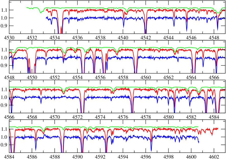
Figure 1: An example of subtraction of the secondary in an SB2 system. The figure shows the original spectrum of HD 103578 in the 4530 Å window (middle spectrum, displaced upwards by 0.1 for clarity); the spectrum of HD 108642 renormalised and pixel-shifted to match the secondary in the HD 103578 system as well as possible (top spectrum, shifted upwards from initial spectrum by 0.03); and the final spectrum of HD 103578A produced by subtraction of the scaled and shifted spectrum of HD 108642 followed by renormalisation to a continuum value of 1.0 (lower spectrum).

It is clear that this procedure does not ensure an accurate determination of the light contribution of the secondary to the total composite spectrum, but only an estimate of this contribution. However, the uncertainty arising from this effect (essentially in the determination of the zero point of the flux in the extracted primary spectrum) is not very large. Typically it is found that the secondary template star contributes about 10% of the light to the composite. Since the lines of the template stars, which always fit the profiles of the secondary star rather accurately, are virtually unbroadened by rotation and therefore quite deep (the Ba II line at 4554.03 Å descends to below 0.2 of the continuum), the amount of light contributed by the secondary will not be overestimated by more than about 10% at the worst, or about 1% of the total flux in the composite spectrum. Similarly, if we assume that the secondary in the composite SB2 spectrum has at least roughly solar composition, its strongest lines, which are highly saturated, should be about as deep as those of the template spectrum. Again, it appears that a 10% underestimate of the secondary’s contribution to the total light is unlikely, which again leads to an overall uncertainty after subtraction of roughly 1% of the continuum in the residual spectrum. This is comparable to the uncertainty caused by correction for scattered light in the composite spectrum, and will not lead to a substantially increased error in either abundance determinations or in the microturbulence parameter $\xi$.

The case of HD 114330 requires individual discussion. From speckle observations there is a visual secondary about 0.45 arcsec from the primary, approximately 2 mag fainter than the primary, and of similar or slightly higher $T_{\mathrm{e}}$ (e.g. Ten Brummelaar et al. TenBetal00 (2000)). However, there is no trace of this component in the observed spectrum. Because image slicers were used in both spectrographs with which data were obtained for this project, light from this component almost certainly is part of the observed spectrum. Thus we suspect that the secondary spectrum is absent either because its lines are extremely broad, or because they are extremely narrow and coincide with those of the primary. We see no trace of broad lines in our (blue) spectra, so most probably the lines of the secondary are very narrow, and we must be concerned about how they influence our analysis. If weak secondary lines are present on the blue wing of each primary line, these contaminating lines could perhaps produce excess blue wing absorption in strong lines (or in most lines), and line profiles that do not closely match computed ones. It is not clear that such contamination could lead to strong lines that require a larger value of $v_{\mathrm{e}}\sin i$ for best fit compared to weak lines. Clearly, caution must be exercised in interpreting spectra of HD 114330, and our conclusions cannot rest on this star alone.

4 Modelling of spectra with ZEEMAN

To uncover the information encoded in the observed spectral lines of a star about the atmospheric velocity field(s) present, we must compare the observed spectrum to a computed spectrum which incorporates some model velocity fields, typically thermal broadening, the rotational velocity $v_{\mathrm{e}}\sin i$, and the standard model of height-independent Gaussian microturbulence. The first step in this process, so that we can select an (approximately) appropriate atmosphere model from a precomputed grid of ATLAS 9 solar composition models (Kurucz Kuru79 (1979), Kuru92 (1992)), is to determine the effective temperature $T_{\mathrm{e}}$ and gravity $\log g$.

These parameters were determined using available Strömgren $uvby{\rm H}\beta$ and Geneva six-colour photometry, together with appropriate calibrations. Temperatures determined using the two different photometry systems usually agree within roughly 1% (typically 100 K at $T_{\mathrm{e}}\sim 10^{4}$ K), although of course the absolute values of $T_{\mathrm{e}}$ are probably only known to within 2–3%. The agreement of the inferred values of $\log g$ was worse, typically 0.2–0.3 dex, presumably because the Geneva system does not have a narrow-band filter equivalent to the H$\beta$ filter of the Strömgren system, and thus is less sensitive to gravity (for hot stars) and more sensitive to interstellar reddening (for cool stars). We generally adopted a value of $\log g$ close to the value given by the Strömgren calibration.

For SB2 stars, approximate values of $T_{\mathrm{e}}$ and $\log g$ were found using the combined light. We tried to improve these values by varying the assumed values of $T_{\mathrm{e}}$ and $\log g$ to see if the quality of the fit to our spectral windows was significantly improved by a somewhat different choice of these fundamental parameters, but for all the stars of interest we were unable to determine more accurately the fundamental parameters of the primary star from our short spectra. We therefore retained the estimates obtained using the combined light, which in general probably yield values of $T_{\mathrm{e}}$ that are slightly too high, perhaps by 1–2%.

The observed spectra of the stars in our sample have been modelled using the FORTRAN programme zeeman.f (version zabn4.f), described by Landstreet (jdl88 (1988)) and Landstreet et al. (Landetal89 (1989)), and compared to other magnetic line synthesis codes by Wade et al. (Wadeetal01 (2001)). This is nearly the same programme that was used in the previous study of line profiles of sharp-line A and B stars by Landstreet (jdl98 (1998)) except for extensive modifications to include the effects of anomalous dispersion for a stellar atmosphere permeated by a magnetic field. These modifications have essentially no impact on the analysis of the present (non-magnetic) stars.

Zeeman.f makes extensive use of spectral line data obtained from the Vienna Atomic Line Database (Kupka et al. Kupetal00 (2000), Kupetal99 (1999); Ryabchikova et al. Ryaetal97 (1997); Piskunov et al. Pisetal95 (1995)).

A key feature of this programme is that it can be instructed to search for an optimum fit to a single chemical element in one (or several) observed spectra; at the same time, it finds the best fit radial velocity for the spectrum, and the best fit value of $v_{\mathrm{e}}\sin i$. This fitting is done assuming the standard model of height-independent Gaussian microturbulence, and the fitting sequence can be carried out for a series of different values of microturbulence parameter $\xi$ to enable the best fitting $\xi$ to be selected. The programme returns the value of the $\chi^{2}/\nu$ of the best fit ($\nu$ is the number of degrees of freedom of the fit), as well as the parameters of the best fit.

Zeeman.f can be used in several somewhat different modes. Two modes were mostly used in this study. In one, we optimise the fit to an element using all the significant lines of that element in one entire observed spectrum (30 to 75 Å long), for a series of values of $\xi$, selecting in the end the value of $\xi$ which fits the spectrum best, and the corresponding abundance. This method only leads to a determination of $\xi$ if the spectrum includes spectral lines having a range of strengths, at least some of which are saturated. If all the spectral lines are relatively weak, different values of $\xi$ fit the spectrum roughly equally well, up to the value at which microturbulence broadens the line by more than its total observed width.

In the second mode, we optimise the fit of a set of selected spectral lines of one element, one line at a time (i.e. in short windows, typically 1–2 Å wide, around each of the selected lines), as a function of $\xi$, and then plot ”Blackwell diagrams” (Landstreet jdl98 (1998)): inferred abundance as a function of $\xi$ for each spectral line separately. If some of the spectral lines used are fairly saturated while others are weak, the resulting curves will usually intersect in a well-defined small region, which determines both the best fitting abundance of the element, and the best fit value of $\xi$. The programme output using this method allows us to examine conveniently the quality of the fit of an individual model spectral line to a particular observed line as a function of the various parameters such as $v_{\mathrm{e}}\sin i$ and $\xi$, and makes it easy to see whether or not the same fitting parameters are derived from all spectral lines of one (or several) element(s). Some Blackwell diagrams are shown by Landstreet (jdl98 (1998)).

The available high-quality spectra for each star have been analysed as described above. In general, we have optimised abundances of the principal detectable elements (some of He, O, Si, Ti, Cr, Fe, Ni, Zr, Ba) as a function of the microturbulence parameter $\xi$, and chosen the microturbulence parameter value which yielded the best concordance of abundances derived from different spectral lines of one to three elements (usually Ti, Cr, and Fe, and sometimes Si) for which enough lines, with a large enough range of equivalent width, are available. The deduced value of $\xi$ is then used to determine abundances of all other elements.

The best-fit values of $v_{\mathrm{e}}\sin i$ and $\xi$, and the abundances of Si, Cr, and Fe, with our estimates of uncertainties, are reported in Table 1. In cases where the available range of line strengths in our spectra was not sufficient to allow us to determine the value of $\xi$ we report “nd $\pm$ nd” (for “not detected”). In a number of stars we were only able to obtain upper limits to the values of $\xi$, usually from Blackwell diagrams, but occasionally from the very narrow line profiles; such cases are reported with equal values and uncertainties for $\xi$ (e. g. $0.5\pm 0.5$ $\mathrm{km\,s}^{-1}$).

Abundances are given as logarithmic number densities relative to H, because this is essentially what we measure; for many stars in our sample the atmospheric abundance of He is unknown (and probably not close to solar), so we prefer to report $\log(n_{X}/n_{\rm H})$ rather than $\log(n_{X}/n_{\rm tot})$ values, which requires an ad hoc assumption about $n_{\rm He}/n_{\rm H}$. Uncertainties in the quoted abundance values are due in part to fitting uncertainties, which arise because abundances derived from individual spectral lines for a given value of $\xi$ always show some scatter about the average, due to imprecise atomic data (especially $gf$ values), to the fact that we do not have a correct model of strong lines with which to fit the observations, and to the fact that the atmosphere model used is only an approximate description of the actual stellar atmosphere. These fitting uncertainties are typically of the order of 0.1 dex in size. There is an additional uncertainty from the fact that the fundamental parameters of each star are only known with a limited precision. We assume that the value of $T_{\mathrm{e}}$ has an accuracy of approximately $\pm 3$%, and that $\log g$ is known to about $\pm 0.25$ dex. We have carried out a number of experiments to test the effect of these uncertainties on the derived abundances, by rederiving abundance values after changing $T_{\mathrm{e}}$ or $\log g$. Because our abundances are generally obtained from the dominant ion, the abundances are not very sensitive to changes in either $T_{\mathrm{e}}$ or $\log g$. The uncertainties in fundamental parameters change the derived abundances by an amount which varies from element to element but is of the order of 0.1 dex. The total uncertainty given for each abundance in Table 1 is then the sum in quadrature of the individual fitting uncertainty and a fixed uncertainty of 0.1 dex arising from fundamental parameter uncertainties.

Note also that since we do not model macroturbulence, but include all broadening except for instrumental, thermal, and microturbulent in our $v_{\mathrm{e}}\sin i$ broadening, the values of $v_{\mathrm{e}}\sin i$ for the coolest stars of our sample are larger than those given in studies which separate the rotational and macroturbulent components of line broadening.

For the stars with the sharpest lines, the precise value of $\xi$ obtained by our fitting procedure may not be the same as the value found by other methods, even with the same observational material and atomic data. This is because we fit line profiles using a $\chi^{2}$ minimisation procedure rather than fitting equivalent width. As will be seen below (and was discovered by Landstreet jdl98 (1998)), for the sharp-line A stars the standard line profile model with microturbulence does not fit the profiles of some very strong lines at all well, effectively showing that this is an inadequate description of these lines. In this situation, it is not clear that there is any good reason to prefer one fitting method over the other – but it may well be that in some cases they yield slightly different values of $\xi$.

We have compared the basic parameters we have chosen for stars analysed, and the resulting abundance values, with a number of previous analyses available in the literature (e.g. Hill & Landstreet HillLand93 (1993); Adelman et al. Adeletal97 (1997); Hui-Bon-Hoa Hui00 (2000); Pintado & Adelman PintAdel03 (2003); Gebran et al. Gebretal08 (2008)). In most cases our value of $T_{\mathrm{e}}$ is within about 200 K, and our $\log g$ within about 0.2 dex, of values adopted by other authors. Our values of $\xi$ are mostly in agreement to within 0.5 $\mathrm{km\,s}^{-1}$ or less, and our resulting element abundances agree within $\pm 0.2$ dex. These discrepancies are fairly typical for the differences between independent abundance analyses of B and A stars, and probably derive from differences in fundamental parameters, detailed model atmospheres used, choices of $gf$ values and wavelength regions, etc. The only significant systematic disagreement we find is that the element abundances we derive for the supergiants in our sample are almost always of order -0.3 dex lower than the LTE abundances found by Venn (Venn95 (1995)). The origin of this difference has not been identified, but does not affect the analysis of spectral line profiles which is the main subject of this paper.

5 Evidence of atmospheric velocity fields

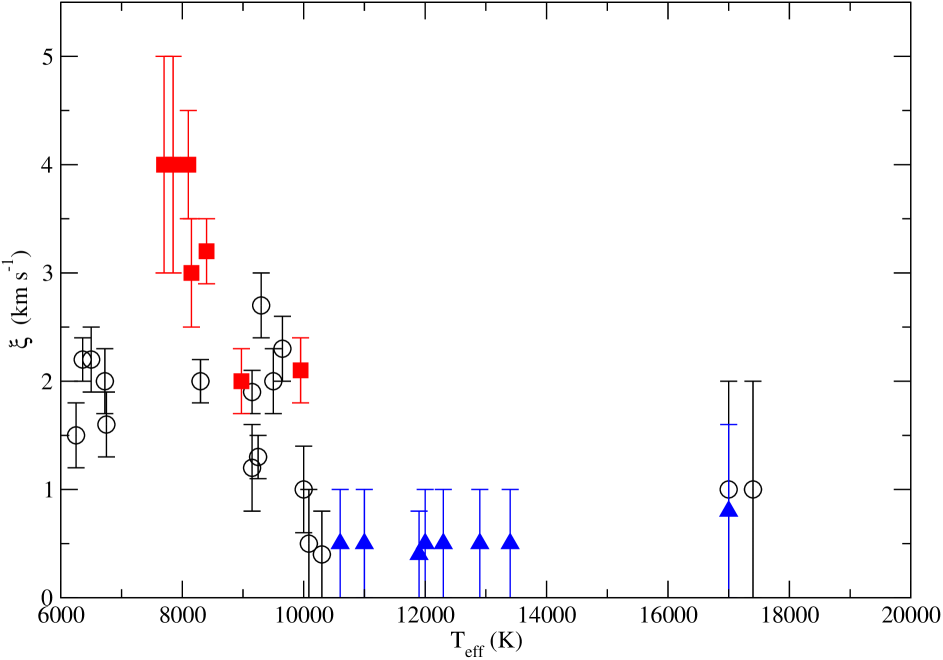
Figure 2: Microturbulence parameter $\xi$ as a function of stellar $T_{\mathrm{e}}$ for main sequence stars in the sample. Open symbols are normal stars, filled squares are Am stars, and filled upright triangles are HgMn stars.

In our previous study of atmospheric velocity fields in middle main sequence stars (Landstreet jdl98 (1998)), several kinds of observational evidence of velocity fields were studied: strong lines whose profiles departed significantly from those predicted by the standard microturbulence model; significant (in some cases quite strong) excess absorption in the blue wings of strong lines; deduced rotation velocities $v_{\mathrm{e}}\sin i$ which increase with line equivalent width; and the microturbulence parameter $\xi$. Microturbulence has been known and studied for decades, but the other spectral line symptoms of local velocity fields were systematically studied in tepid main sequence stars for the first time in our previous study.

One of the results of the spectrum synthesis carried out for the stars of this sample is a determination of the microturbulence parameter $\xi$ (see Table 1) for all the stars of the sample except a few hot stars that have no saturated lines in the window(s) observed. The derived values of $\xi$ are plotted as a function of stellar effective temperature $T_{\mathrm{e}}$ in Figure 2, with separate symbols for normal, Am, and HgMn stars. This figure clearly shows the expected behaviour: $\xi$ is zero within the uncertainties for $T_{\mathrm{e}}\geq 10\,000$ K, while below this temperature it rises rapidly towards lower $T_{\mathrm{e}}$ to a limiting value which for most stars is approximately 2 $\mathrm{km\,s}^{-1}$.

The peculiar stars of this diagram have quite distinctive behaviour. In none of the Ap HgMn stars is a non-zero value of $\xi$ detected, consistent with models of these stars that require vertically stratified atmospheres (e.g. Sigut Sigu01 (2001)). In contrast, all the metallic-line Am stars have clearly non-zero values of $\xi$. For the hotter Am stars ($T_{\mathrm{e}}\geq 8\,500$ K), the value of $\xi$ is indistinguishable from that of normal stars of the same $T_{\mathrm{e}}$ value, but the cooler Am stars tend to have $\xi$ values about 1 to 2 $\mathrm{km\,s}^{-1}$ larger than the values found for normal stars. The relatively large $\xi$ values found for the five cool Am stars of the present sample are consistent with the results of Landstreet (jdl98 (1998)) for a smaller sample.

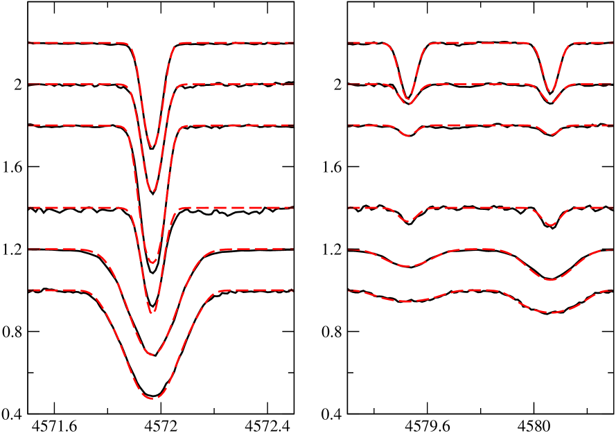
Figure 3: At most very weak convection signatures in spectral lines of stars with $T_{\mathrm{e}}$ values between 13000 and 9000 K observed in the 4530 – 4600 Å window. From top to bottom, in order of decreasing $T_{\mathrm{e}}$: HD 186122 (46 Aql), HD 178065, HD 175640, HD 181470A, HD 214994 (o Peg, exceptionally observed only with $R=40\,000$), and HD 73666. The top three stars are late B HgMn stars, while the lower three stars are normal A stars (one of which is an SB2). The solid lines show the observed line profiles of the strong 4571.97 Å line of Ti ii (left panel) and two weak to moderate lines of Fe ii at 4579.53 and 4580.06 Å (right panel); the dashed lines show profiles computed with the standard line model of depth-independent, isotropic microturbulence, using the parameters of Table 1.

The most striking symptom of atmospheric velocities discovered by Landstreet (jdl98 (1998)) was the large departure of the line profiles of strong spectral lines in a few stars from the profiles predicted by the standard model of a height-independent, isotropic Gaussian (microturbulent) velocity field. The velocity field signature takes the form of line profiles of strongly saturated lines that are much more triangular than line profiles predicted by the standard model. Furthermore, these strong lines have substantial excess absorption in the blue line wing relative to synthetic line profiles. Such pointed, asymmetric profiles are reminiscent of the line profiles found in slowly rotating cool stars, which are modelled by introducing macroturbulence. It is clear that such line distortions signal the presence of local atmospheric motions more complex than those assumed by the standard microturbulent model, and provide valuable information about these motions.

Table 2: Main sequence A-type stars in which evidence of velocity fields is directly detected in line profiles

HD	other	spectral	binarity	$T_{\mathrm{e}}$	$\xi$	depressed	line shape	$v_{\mathrm{e}}\sin i$
		type				blue wing	discrepancy	weak lines	strong lines
				(K)	($\mathrm{km\,s}^{-1}$)			($\mathrm{km\,s}^{-1}$)	($\mathrm{km\,s}^{-1}$)
2421 A	HR 104 A	A2Vs	SB2	10000	1.0	weak	none	3.5	3.5
72660	HR 3383	A1V		9650	2.3	weak	weak	5.0	6.1
114330	$\theta$ Vir	A1Vs	VB2	9250	1.3	weak	weak	4.0	5.5
157486 A	HR 6470 A	A0V	SB2	9150	1.9	weak	weak	1.5	3.5
27962	68 Tau	A2IV m	SB1	8975	2.0	weak	weak	11	11.5
103578 A	95 Leo A	A3V	SB2	8300	2.0	strong	strong	3	9
107168	8 Com	A8 m		8150	3.0	weak	weak	13	14
108642 A	HR 4750 A	A2 m	SB1	8100	4.0	strong	strong	2	10
209625	32 Aqr	A5 m	SB1	7700	4.0	strong	strong	4.5	10

In the previous study, the phenomenon was only observed in very clear form in two stars (HD 108642 and HD 209625) with $T_{\mathrm{e}}$ values close to 8000 K, both of which are Am stars. One further normal early A star (HD 72660) was found to show a very attenuated departure of observed line profiles from computed ones, primarily in the form of observed blue line wings that are slightly depressed below the computed line wings. For the other two stars in that study with $T_{\mathrm{e}}$ below 10 000 K, the $v_{\mathrm{e}}\sin i$ values are too large for a significant departure from a purely rotational profile to be seen. All observed line profiles of three very sharp-line stars hotter than $T_{\mathrm{e}}\approx 10\,000$ K were found to be in very good agreement with the computed profiles; no indication of any atmospheric velocity field other than bulk stellar rotation is seen in the lines. As discussed in the introduction, the main goals of the present project are to find more examples of such line profile discrepancies, to discover whether the phenomenon is restricted essentially to Am stars, or is found more generally, and to determine more clearly over what range of $T_{\mathrm{e}}$ directly observable velocity field symptoms are found.

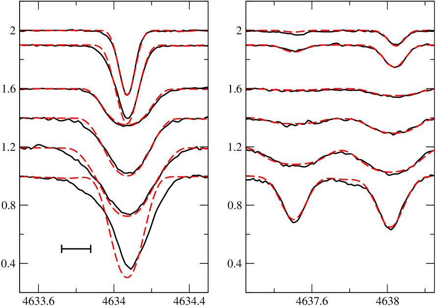
Figure 4: Convection signatures (particularly the depressed blue line wing) in spectral lines of stars with $T_{\mathrm{e}}$ in the range 10000 to 7500 K, observed in the 4615 – 4645 Å window. From top to bottom, in order of decreasing $T_{\mathrm{e}}$: HD 2421A, HD 72660, HD 47105, HD 27962, HD 107168, and HD 209625. The top three stars are normal A stars, while the lower three stars are all Am stars. The solid lines show the observed line profiles of the strong 4634.07 Å line of Cr ii (left panel) and the weak 4637.50 Å line of Fe i and the blend of 4638.01 Å of Fe i and 4638.05 Å of Fe ii (right panel); the dashed lines show profiles computed with the standard line model of depth-independent, isotropic microturbulence, using the parameters of Table 1. The bar in the lower left corner of the left panel represents a wavelength shift equivalent to 10 $\mathrm{km\,s}^{-1}$.

In Figures 3 through 5 we compare the result of detailed modelling of lines of the sharpest-lined main sequence stars in the present sample with observed line profiles. Two spectral windows are shown, reflecting the available observational material for the stars of the sample: data in the window around 4560 Å were obtained in 2000–01, while data in the window around 4630 Å are from earlier observing runs. In each figure, the line in the left panel is the strongest spectral line in the observed window that is essentially free from blends in the range of $T_{\mathrm{e}}$ of the figure. The right panel shows a relatively weak line that is also largely blend-free. These observed lines are compared with model spectral lines computed assuming the standard model of velocity broadening due to the atomic thermal velocities, depth-independent, isotropic Gaussian microturbulence, and rigid-body rotation, along with appropriate instrumental broadening.

As mentioned above, in stars showing significant line asymmetry, it is also found that the $v_{\mathrm{e}}\sin i$ value that best fits the strongest lines is almost always significantly larger (by up to several $\mathrm{km\,s}^{-1}$) than that which best fits the weakest lines. Presumably this effect reflects the extra contribution of the local macroscopic velocity field to the line width of saturated lines, and the true value of $v_{\mathrm{e}}\sin i$ is (at most) as large as the minimum value found using the weakest, sharpest lines. In the figures, the projected rotational velocities of the synthetic lines with which these observed lines are compared are determined using only the weakest lines, and the same $v_{\mathrm{e}}\sin i$ value is used for all lines of each star. The value of $\xi$ used is the value reported in Table 1, derived from the abundance modelling of weak and strong lines.

These three figures clearly display the same phenomena identified by Landstreet (jdl98 (1998)): no trace of macroscopic velocity fields above about 10 000 K, while below that temperature $\xi$ rises rapidly from zero, and particularly sharp-lined stars show $v_{\mathrm{e}}\sin i$ values that depend on line strength, line asymmetries, and significant discrepancies between computed and observed line profiles of strong lines.

For each of the four stars in Figure 3 with effective temperatures above about 10 000 K (HD 186122, 178065, 175640, and 181470A, the first three of which are Ap HgMn stars), the value of $\xi$ is not significantly different from zero. The same value of $v_{\mathrm{e}}\sin i$ fits weak and strong lines, and in all cases the fit is very good to both weak and strong lines, which are clearly symmetric. These stars show no significant trace of local large-scale velocity fields such as “macroturbulence”. The same result was found for the normal star HD 209459 = 21 Peg ($T_{\mathrm{e}}=10200$ K) by Landstreet (jdl98 (1998)).

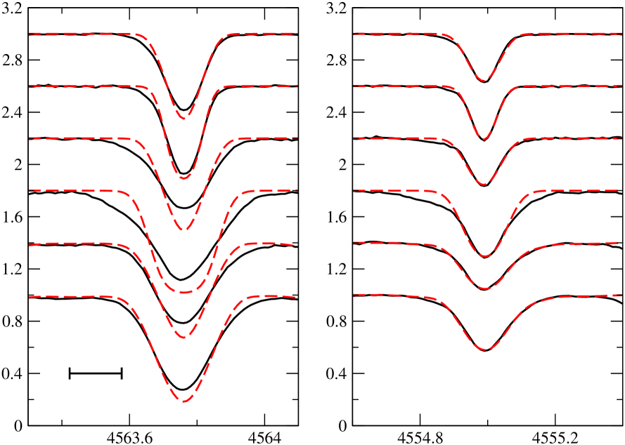
Figure 5: Convection signatures in spectral lines of stars with $T_{\mathrm{e}}$ in the range 9250 to 6500 K, observed in the 4530 – 4600 Å window. From top to bottom: HD 114330, HD 157486A, HD 103578A (95 Leo A), HD 108642A, HD 185395 ($\theta$ Cyg), and HD 61421 (Procyon). The top star is a normal A star, the next two stars are normal (SB2) A stars, the fourth star is an Am star, and the bottom two are normal F stars. The solid lines show the observed line profiles of the strong 4563.76 Å line of Ti ii (left panel) and the weak to moderate 4554.99 Å line of Cr ii (right panel); the dashed lines show profiles computed with the standard line model of depth-independent, isotropic microturbulence, using the parameters of Table 1. The bar in the lower left corner of the left panel represents a wavelength shift equivalent to 10 $\mathrm{km\,s}^{-1}$.

Of the seven stars in these figures with $T_{\mathrm{e}}$ between 9 000 K and 10 000 K, the four with $v_{\mathrm{e}}\sin i$ below 6 $\mathrm{km\,s}^{-1}$ (HD 2421A, HD 72660, HD 114330, and HD 157486A) show small but clear deviations from the synthesized line profiles, specifically depression of the observed blue line wing relative to the computed line for the strong (but not the weak) lines. In contrast, the two stars with $v_{\mathrm{e}}\sin i\sim 10$ $\mathrm{km\,s}^{-1}$ (HD 73666 and 47105), and the one star of $v_{\mathrm{e}}\sin i=7$ $\mathrm{km\,s}^{-1}$ observed with $R=40\,000$ show no detectable effect, even though their $\xi$ values are comparable to those of HD 2421 and HD 157486; for these stars the small velocities of the local velocity field are concealed by the rotational and/or instrumental broadening.

There are six sharp-line stars in the sample with $T_{\mathrm{e}}$ in the range 7 500 to 9 000 K: HD 27962, HD 103578A, HD 107168, HD 108642, HD 189849, and HD 209625. (Two of these are the two Am stars studied by Landstreet jdl98 (1998).) In this temperature range the local velocity field amplitude is large enough to be clearly visible even with $v_{\mathrm{e}}\sin i$ above 10 $\mathrm{km\,s}^{-1}$ (HD 27962 and 107168, but not in HD 189849 for which our observational material is of low quality), and, as previously found, in stars with sharper lines the impact of the local velocity field is really striking. In HD 103578A, 108642 and 209625 the deviations from the model are clearly visible even in the weak lines used to determine $v_{\mathrm{e}}\sin i$. In these stars the discrepancy between the calculated and observed line profiles is very substantial for the strong lines, both in the core shapes and in the occurrence of observed blue line wings that are shallower and deeper than the computed ones. In HD 27962 and 107168, both of which have $v_{\mathrm{e}}\sin i$ values above 10 $\mathrm{km\,s}^{-1}$, the effects are visible but not striking.

Finally, we also show two F stars in Figure 5 whose $T_{\mathrm{e}}$ values are below 7 000 K (HD 185395 and HD 61421), and which show the well-known shape discrepancies of solar-type stars in the strong lines, with the red line wings of the strong observed lines shallower than and depressed below the model profile. Note that the line profiles of A-type stars with depressed blue wings as shown in Figure 5 are very different from the blueward hook phenomenon which has been observed for F-type stars such as Procyon and explained to originate from saturation of strong lines in upflow regions (Allende Prieto et al. Prieetal02 (2002)). The cool star blueward hook feature only affects lines close to their continuum level and is much smaller in terms of velocities (less than 0.5 $\mathrm{km\,s}^{-1}$).

To provide a scale for the velocity amplitude required to account for the line profile distortions, in each figure where these effects are apparent we include a small horizontal error bar with a total width of 10 $\mathrm{km\,s}^{-1}$.

A summary of all the main sequence A stars in which we find direct evidence of an atmospheric velocity field (beyond that provided by a non-zero value of $\xi$) has been found is given in Table 2. Columns 3 to 6 recall the spectral type, binarity, effective temperature and microturbulence parameter of these stars. In the column “depressed blue wing” the comment “weak” or “strong” indicates the extent to which the short-wavelength line wing is deeper than the long-wavelength wing. The column “line shape discrepancy” describes qualitatively the extent of discrepancies, other than the depressed blue line wing, between observed and calculated line profiles of the strongest spectral lines. The last two columns list extreme values of $v_{\mathrm{e}}\sin i$ as derived from best fits to the weakest and strongest spectral lines in our spectra. As discussed qualitatively above, we see that the difference between the best fit $v_{\mathrm{e}}\sin i$ values for the weakest and strongest lines in our spectra seems to increase quite rapidly for $T_{\mathrm{e}}$ below about 9000 K to a value that can be several $\mathrm{km\,s}^{-1}$ at around 8000 K. (Note that HD 3883, noted by Gray & Nagel [gn89 (1989)] as having a reversed bisector, is omitted from Table 2 because we have no spectra of this star.)

We notice that the direct evidence of velocity fields in the line profiles agrees very well with the indirect evidence provided by the microturbulence parameter. Main sequence stars having $T_{\mathrm{e}}$ above about 10000 K have $\xi$ values that are indistinguishable from 0, and thus lack any evidence of small-scale velocity fields. These same stars have spectral lines that are in excellent agreement with calculated line profiles in which the broadening is assumed to be due only to rotation, thermal broadening, collisional damping, and instrumental resolution; these stars thus do not show any direct evidence of local atmospheric hydrodynamic motions.

In contrast, stars with $T_{\mathrm{e}}$ below 10000 K all have non-zero values of $\xi$, and all the stars with “sufficiently” small values of $v_{\mathrm{e}}\sin i$ also show direct line profile evidence of velocity fields. Local velocity fields are detectable through differences between profiles of observed strong spectral lines and computed lines, through asymmetries in the observed lines, and in most cases through best-fit $v_{\mathrm{e}}\sin i$ values that are systematically larger for strong than for weak lines. Furthermore, the strongest directly detected symptoms of local velocity fields, observed in stars with $T_{\mathrm{e}}$ around 8000 K, generally coincide with the largest deduced values of $\xi$.

These results confirm the findings from a smaller dataset by Landstreet (jdl98 (1998)), where it was shown that the range of effective temperatures for which non-zero-values of $\xi$ are found coincides rather closely with the occurrence of a convectively unstable region in the stellar atmosphere as predicted by the Schwarzschild criterion applied to the model atmosphere used for spectrum synthesis. Thus, the occurrence of convective motions in the atmospheres is expected in essentially the range of $T_{\mathrm{e}}$ in which it is observed. The importance of the observations presented in this paper comes from the direct signatures of this convection in spectral lines, which should be able to provide significant constraints on the nature of the actual flows occurring in the atmosphere.

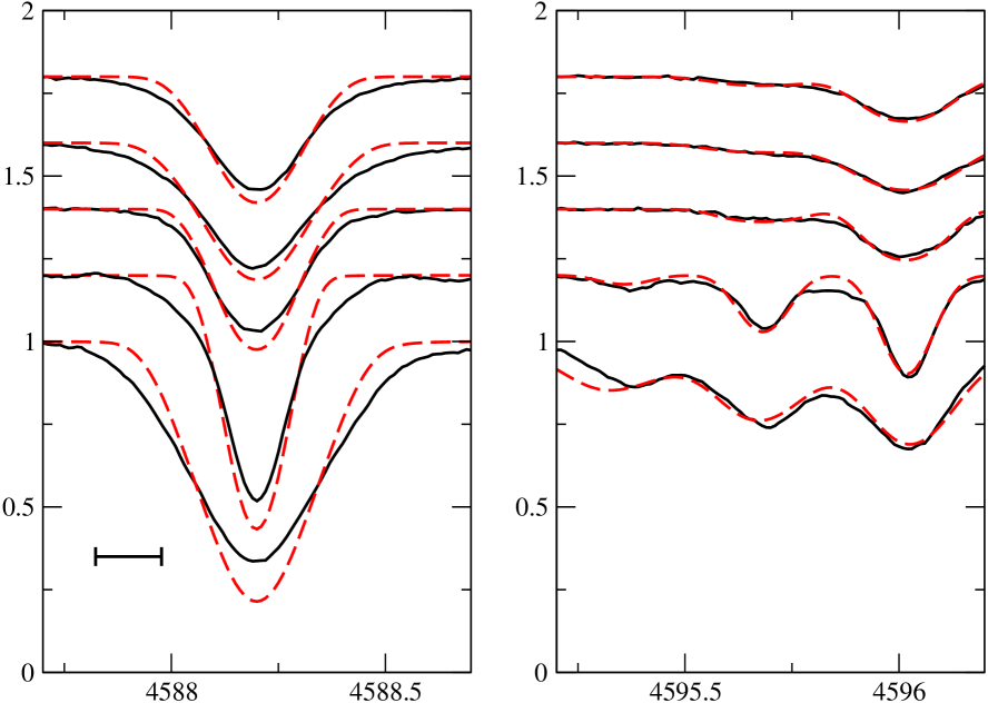
Figure 6: Striking convection signatures in spectral lines of A and early F-type supergiants with $T_{\mathrm{e}}$ values between 9700 and 6800 K observed in the 4530 – 4600 Å window. From top to bottom: HD 46300 (13 Mon), HD 87737 ($\eta$ Leo), HD 175687 ($\xi^{1}$ Sgr), HD 147084 (o Sco), and HD 182835 ($\nu$ Aql). The solid lines show the observed line profiles of the strong 4588.20 Å line of Cr ii (left panel) and a group of weak to moderate lines, 4595.36 and 4596.06 Å of Fe i and 4595.68 and 4596.02 Å of Fe ii (right panel); the dashed lines show theoretical profiles computed with the standard line model of depth-independent, isotropic microturbulence computed with the parameters of Table 1. The bar in the lower left corner of the left panel represents a wavelength shift equivalent to 10 $\mathrm{km\,s}^{-1}$.

It may be noted that the line profile distortions relative to the canonical model are observed essentially only in lines of once-ionised atoms such as Fe, Cr and Ti, and not in the few visible lines of neutral atoms. This is presumably due to the fact that all neutral lines are relatively weak, while the effects we are interested show themselves in strong, heavily saturated lines.

It is of interest to compare the symptoms of local velocity fields found in the spectra of main sequence stars with those found in lines of supergiants of similar spectral types, and for this reason several of the stars in our survey are such luminous objects. It is well known that A and F supergiants require relatively large values of the microturbulence parameter (typically several $\mathrm{km\,s}^{-1}$) for successful spectrum synthesis (e. g. Venn Venn95 (1995); Gray et al. Grayetal01 (2001); Przybilla et al. Przyetal06 (2006)), and so we expect to find strong evidence of velocity fields in the line profiles of the slowest rotators.

Five supergiants, ranging in $T_{\mathrm{e}}$ from 9700 to 6800 K, are listed in Table 1 and are shown in Figure 6. As with the main sequence stars, the $v_{\mathrm{e}}\sin i$ values have been determined using only the weakest lines, and for each star the same value of $v_{\mathrm{e}}\sin i$ has been used for all synthesized profiles. A systematic result of our use of only the weakest lines is that the $v_{\mathrm{e}}\sin i$ values determined here are always significantly smaller than those found in previous studies, where $v_{\mathrm{e}}\sin i$ is fit mainly to the stronger lines. In the right panel of the figure an example of relatively weak lines shows that these profiles are fairly well fit by simple rotational broadening (together with thermal and instrumental broadening and classical microturbulence). In contrast, the observed strong lines of the left panel are all significantly different in shape from the computed lines. If we had (unphysically) allowed $v_{\mathrm{e}}\sin i$ to be a free parameter for each spectral line separately, the strong lines could have been substantially better fit. In each case the best fit $v_{\mathrm{e}}\sin i$ value determined from strong lines is a few $\mathrm{km\,s}^{-1}$ larger than that found from weak lines, and is similar to values found in other high-resolution studies. In the coolest star shown, HD 182835, the best fit $v_{\mathrm{e}}\sin i$ value found from weak lines is no more than 10 $\mathrm{km\,s}^{-1}$, while the best fit for the strongest lines is about 18 $\mathrm{km\,s}^{-1}$!

Thus, we find in these highly luminous stars evidence for the local velocity fields phenomenologically similar to that found in main sequence stars of similar $T_{\mathrm{e}}$, but with larger amplitude. However, there is one significant difference: the supergiants do not show the strong line asymmetry seen in the main sequence stars with similar temperatures. The depression of the observed wings of strong lines below the computed wings is essentially the same on the blue and red sides of the line. This result is different from that of Gray & Toner (GrayTone86 (1986)), who find significant excess absorption in the blue wings of spectral lines of F supergiants. However, their data suggest that the asymmetry diminishes towards earlier spectral types. As their earliest supergiant has spectral type F5 while our latest type is F2, perhaps we are simply seeing the asymmetry decrease below the threshold for easy visibility.

A different possibility for the velocity field observed in supergiants is that the line profiles reveal the presence of pulsations. Aerts et al. (Aertetal08 (2008)) have shown that the qualitatively similar line profiles of an early B-type supergiant, typically modelled by macroturbulence, may be produced by numerous low-amplitude gravity-mode oscillations, rather than by large-scale convective motions.

This raises the question of whether the velocity fields that we observe in sharp-line A-type main sequence stars might also be due to pulsations, but there are several reasons to doubt this. The first is that the computations of Aerts et al. (Aertetal08 (2008)) do not show any significant line asymmetry, the most persistent feature we observed in the line profiles of A stars. Furthermore, we observe depressed blue line wings and other symptoms of a velocity field in stars significantly hotter than the hot limit of the instability region (about 8700 K or a bit cooler; e.g. Joshi et al. Joshetal03 (2003)). A third reason for rejecting pulsations is that the asymmetry of line profiles in tepid stars has a constant behaviour, reproducible through repeated observations of all the stars in Table 2: the excess absorption is always in the short-wavelength line wing. It is difficult to see why pulsation would not lead to excess absorption that would shift from one line wing to the other. Finally, one of the stars in which the symptoms of a non-thermal velocity field are strongest, HD 209625, has been observed very carefully to search for evidence of pulsations (Carrier et al. Carretal07 (2007)), but no hint of pulsational variations was found. This is consistent with many observational studies which have concluded that only marginal and evolved Am stars are found to pulsate (cf. the review of Balona Balo04 (2004)), thus supporting theoretical results from diffusion theory (Turcotte et al. Turcetal00 (2000)). A few exceptional classical Am stars, pulsating at very low amplitude, have nevertheless been identified (Kurtz Kurt00 (2000)). In contrast, not all the normal A stars in the centre of the instability strip are found to pulsate above observational thresholds and $\delta$ Sct variables with low $v_{\mathrm{e}}\sin i$ are found to have a very large spread in observed pulsation amplitudes (Breger Breg00 (2000)). Thus, although we cannot completely exclude pulsation from being present in the stars listed in Table 2 with $T_{\rm e}\leq 8700$ K, their maximum variability level due to pulsation has to be very small, making pulsation a very unlikely candidate for large velocity fields that cause asymmetrically broadened line profiles.

It is of course possible to consider other explanations of the depressed line wings than atmospheric motions. The excess broadening is not caused by magnetic (Zeeman) broadening, as this would selectively broaden lines of large Zeeman sensitivity; instead one finds simply that all the strongest lines are broadened most. In particular, if the broadening were magnetic, the strong 4634.07 Å line of Cr ii would be considerably narrower than the nearby 4629.34 Å line of Fe ii; this is not observed. Similarly, we can exclude the possibility that the effect is caused by hyperfine splitting, because the principle isotopes of Fe, Cr, and Ti, in which strong line distortion is observed, are overwhelmingly even-even isotopes with no net nuclear magnetic moment, and also because the observed effect depends strongly on stellar $T_{\mathrm{e}}$. We can exclude the possibility that the selective broadening and distortion is caused by rapid rotation seen pole on, as this would broaden both strong and weak lines by a similar amount. We note that also a direct interaction between the two members of each of the observed binaries in the sample is unlikely to explain the asymmetric profiles due to their constant behaviour over different rotational periods and the varied nature of their binarity. Finally, it seems unlikely that circumstellar material (which can have quite large velocities) plays any role, as there is no observed emission at H$\alpha$ and H$\beta$, such as one finds in Herbig AeBe stars.

We conclude that the atmospheric convective velocity field is still the most probable explanation of the line profile peculiarities reported here.

6 Conclusions

The results described in the preceding sections lead to a number of conclusions.

Local atmospheric velocity fields are confidently detected in main sequence stars having $T_{\mathrm{e}}$ below 10000 K, but not in stars with higher effective temperatures. These velocity fields are always detected via clearly non-zero values of the microturbulence parameter $\xi$, which is indistinguishable from zero for $T_{\mathrm{e}}\geq 10000$ K, but rises quickly to a value near 2 $\mathrm{km\,s}^{-1}$for lower $T_{\mathrm{e}}$. A larger value of $\xi$ is found essentially only for Am stars with $T_{\mathrm{e}}$ between 7500 and 9000 K.

In all stars with sufficiently sharp lines ($v_{\mathrm{e}}\sin i$ below about 6 $\mathrm{km\,s}^{-1}$for stars with $9\,000\leq T_{\mathrm{e}}\leq 10\,000$ K, and below about 12 or 13 $\mathrm{km\,s}^{-1}$ for stars with $7\,500\leq T_{\mathrm{e}}\leq 9\,000$ K), there is a perfect correspondence between non-zero $\xi$ and other expressions of a local velocity field. Sharp-line stars with non-zero microturbulence also exhibit some or all of (1) best-fit values of $v_{\mathrm{e}}\sin i$ that increase with the equivalent width of the line, (2) significant line asymmetry, with a deeper depression of the blue line wing for stars with $T_{\mathrm{e}}$ larger than about 7000 K, and a deeper red wing for cooler stars, and (3) profiles of strong lines that are clearly not correctly modelled by the usual LTE line formation theory if one assumes that the only line broadening mechanisms are instrumental broadening, thermal and pressure broadening, height-independent isotropic Gaussian microturbulence, and rotation with $v_{\mathrm{e}}\sin i$ derived from the weakest available lines.

Our search for more stars which clearly exhibit characteristics (2) and (3) has yielded only a few new examples (HD 2421A, HD 27962, HD 103578A, HD 107168, HD 157486A, and probably HD 114330). However, even this small number has tripled the available sample. The line profile characteristics of these stars are consistent with those of the very sharp-line stars already studied (HD 72660, HD 108642A, and HD 209625; Landstreet jdl98 (1998)), both in form and in variation with effective temperature. From the newly detected stars we learn that the modifications to spectral lines produced by local velocity fields are found in both Am and non-Am stars of similar $T_{\mathrm{e}}$, although (consistent with the larger $\xi$ values found in Am stars) the amplitude of line profile distortions seems larger in Am than in normal A stars. The effects directly observable in really sharp-line A-star spectra become stronger as $T_{\mathrm{e}}$ decreases below 10 000 K, down to about 7 000 K, below which the line profiles take on the already well-known shape characteristic of solar-type stars.

There are now sufficient data available to make useful comparison with numerical simulations of convection for an interesting range of values of $T_{\mathrm{e}}$ and $\log g$, and the data for different tepid main sequence stars show a reassuring degree of consistency. We should emphasize that even if the effects we are studying here are observable only in the most slowly rotating stars, they reveal that local line profiles are not predicted correctly by standard theory, and aside from their interest in allowing us to probe the atmospheric velocity fields directly, these effects need to be understood (for example through numerical simulations) so that they can be correctly incorporated into spectrum synthesis codes for determining, for example, abundances in stars of chemical elements for which only saturated spectral lines are available.

It is observed (as is already well-known) that supergiants in this $T_{\mathrm{e}}$ range also show clear symptoms of local velocity fields. These include large non-zero values of $\xi$, best fit $v_{\mathrm{e}}\sin i$ values that increase systematically with equivalent width, and profiles of strong lines that are poorly fit by the canonical line model. However, such stars do not appear to show the line asymmetry found in main sequence A stars, and in the supergiants the line profile distortions may be due to g-mode pulsations (Aerts et al. Aertetal08 (2008)) rather than to local convective velocities.

We conclude by summarising some of the principal observational features that theoretical and numerical models should (and to some extent do) account for.

One major regularity, and one of the strongest pieces of evidence linking the observed line profile shapes to atmospheric convection, is the variation of the strength of the effects discussed here with effective temperature. As $T_{\mathrm{e}}$ rises past about 7000 K, the line profile forms observed change from the solar-type shapes to the shapes observed here, with strongly depressed blue line wings. As $T_{\mathrm{e}}$ continues to rise, the effect becomes steadily weaker until at about $T_{\mathrm{e}}\sim 10\,000$ K the line profiles become indistinguishable from those predicted by the standard model of line shape. As discussed by Landstreet (jdl98 (1998)), this behaviour is completely consistent with the predictions of mixing-length theory. When mixing-length theory is applied to model atmospheres appropriate to main sequence A and late B stars, it is found that the strength of the super-adiabatic temperature gradient in the atmosphere declines rapidly with increasing $T_{\mathrm{e}}$, and its driving effect becomes negligible at about the correct value of $T_{\mathrm{e}}$. Because this behaviour results from a fundamental feature of A and B star atmospheres, namely the decline of continuum opacity as H becomes more fully ionised with rising $T_{\mathrm{e}}$, it is to be expected that it will also be found in numerical models. However, because of the high computational expense of modelling even a single $T_{\mathrm{e}}$ value, this aspect of the velocity field behaviour has not yet been studied numerically; most of the modelling has been done for atmospheres with $T_{\mathrm{e}}$ near 8000 K, where the effects of the super-adiabatic temperature gradient in the lower line-forming region are largest.

The form of profiles of strong lines, with excess absorption far in the blue line wing relative to that in the red wing, represents the most severe challenge to numerical modelling at present. The observations strongly suggest that the integrated form of strong absorption lines is produced by areas of gas rising with relatively large velocity, while the descending gas is moving at a smaller velocity, which presumably (to conserve mass) must cover a larger fractional area. This is the opposite of the solar case, and is still not found in numerical simulations in spite of serious efforts with 2D and 3D codes (e.g. Steffen et al. sfl06 (2006); Kochukhov et al. Kochetal07 (2007)).

A further possible issue arises from the magnitude of the “excess” velocities detected, above line broadening due to thermal motions, pressure broadening, “standard” microturbulence, macroscopic broadening by rotation, and finite spectral resolution. These may be as large as 10 – 12 $\mathrm{km\,s}^{-1}$ as measured by comparing the horizontal discrepancies between observed and computed line profiles. Since the speed of sound is roughly 7.5 to 8.5 $\mathrm{km\,s}^{-1}$ through the line forming region of a main sequence A star, the inferred local velocity field may be significantly supersonic in places. This does not seem to be a real problem, however; Freytag (Frey95 (1995)) and Kupka et al.(Kupketal09 (2009)) both find that shocks occur in their simulations, indicating clearly the local presence of supersonic velocities.

It is very satisfying that line shape observations are able to provide real tests and constraints that challenge efforts to model the detailed behaviour of stellar convection. This confrontation will certainly help to guide theory eventually to a more physically correct description of the phenomenon in stars.

- (1) Abt, H. A., Levato, H., Grosso, M. 2002, ApJ 573, 359
- (2) Abt, H., Morrell, N. I. 1995, ApJS 99, 135
- (3) Adelman, S. J., Caliskan, H., Kocer, D., Bolcal, C. 1997, MNRAS 288, 470
- (4) Aerts, C., Puls, J., Godart, M., Dupret, M.-A. 2008, arXiv:0812.2641
- (5) Allende Prieto, C., Asplund, M., García López, R. J., Lambert, D. L. 2002, ApJ 567, 544
- (6) Asplund, M., Nordlund, Å.; Trampedach, R., Allende Prieto, C., Stein, R. F. 2000, A&A 359, 729
- (7) Balona, L.A. 2004, in The A-Star Puzzle, Eds. J. Zverko, W. W. Weiss, J Ziznovsky, S. J. Adelman (Cambridge, UK: Cambridge University Press) 325
- (8) Breger, M. 2000, in Delta Scuti and Related Stars, Reference Handbook and Proceedings of the 6th Vienna Workshop in Astrophysics, held in Vienna, Austria, 4-7 August, 1999, Eds. M. Breger and M. Montgomery (San Francisco: ASP), 3
- (9) Carrier, F., Eggenberger, P., Leyder, J.-C., Debernardi, Y., Royer, F. 2007, A&A 470, 1009
- (10) Dravins, D., Nordlund, Å 1990, A&A 228, 184
- (11) Freytag, B. 1995, PhD thesis, University of Kiel
- (12) Freytag, B., Steffen, M., Ludwig, H.-G. 1996, A&A 313, 497
- (13) Freytag, B., Steffen, M. 2004, in The A-Star Puzzle, Eds. J. Zverko, W. W. Weiss, J Ziznovsky, S. J. Adelman (Cambridge, UK: Cambridge University Press) 139
- (14) Gebran, M., Monier, R., Richard, O. 2008, A&A 479, 189
- (15) Gray, D. F. 2005, PASP 117, 711
- (16) Gray, D. F., Nagel, T. 1989, ApJ 341, 421
- (17) Gray, D. F., Toner, C. G. 1986, PASP 98, 499
- (18) Gray, R. O., Graham, P. W., Hoyt, S. R. 2001, AJ 121, 2159
- (19) Hill, G. M, Landstreet, J. D. 1993, A&A 276, 142
- (20) Hui-Bon-Hoa, A. 2000, A&AS 144, 203
- (21) Joshi, S., Mary, D. L., Martinez, P., Kurtz, D. W., Girish, V., Seetha, S., Sagar, R., Ashoka, B. N. 2003, MNRAS 344, 431
- (22) Kochukhov, O., Freytag, B., Piskunov N., Steffen, N. 2007, in Convection in Astrophysics, Proceedings IAU Symposium No. 239 Eds. F. Kupka, I.W. Roxburgh & K.L. Chan (Cambridge: Cambridge University Press), 68
- (23) Künzli, M., North, P., Kurucz, R. L., Nicolet, B. 1997, A&AS, 122, 51
- (24) Kupka F., Piskunov N.E., Ryabchikova T.A., Stempels H.C., Weiss W.W. 1999, A&AS 138, 119
- (25) Kupka, F., Ballot, J., Muthsam, H. J. 2009, submitted.
- (26) Kupka F., Ryabchikova T.A., Piskunov N.E., Stempels H.C., Weiss W.W. 2000, Baltic Astronomy, 9, 590
- (27) Kurucz, R. L. 1979, ApJS 40, 1
- (28) Kurucz, R. L. 1992, in “The Stellar Populations of Galaxies: Proceedings of the 149th Symposium of the International Astronomical Union, held in Angra dos Reis, Brazil, August 5-9, 1991. Eds. B. Barbuy & A. Renzini. (Kluwer: Dordrecht) 225
- (29) Kurtz, D. W. 2000, in Delta Scuti and Related Stars, Reference Handbook and Proceedings of the 6th Vienna Workshop in Astrophysics, held in Vienna, Austria, 4-7 August, 1999, Eds. M. Breger and M. Montgomery (San Francisco: ASP), 287
- (30) Landstreet, J.D. 1988, ApJ, 326, 967
- (31) Landstreet, J. D., Barker, P. K., Bohlender, D. A., Jewison, M. S. 1989, ApJ 344, 876
- (32) Landstreet, J.D. 1998, A&A, 338, 1041.
- (33) Levato, H., Malaroda, S., Morrell, N., Solivella, G., Grosso, M. 1996, A&AS 118, 231
- (34) Ludwig, H.-G., Steffen, M. 2008, in “Precision Spectroscopy in Astrophysics, Proceedings of the ESO/Lisbon/Aveiro Conference held in Aveiro, Portugal, 11-15 September 2006. Eds N.C. Santos, L. Pasquini, A.C.M. Correia, and M. Romanielleo (Springer: Berlin) 133
- (35) Napiwotzki, R., Schoenberner, D., Wenske, V. 1993, A&A, 268, 653.
- (36) Pintado, O. I., Adelman, S. J. 2003, A&A 406, 987
- (37) Piskunov N.E., Kupka F., Ryabchikova T.A., Weiss W.W., Jeffery C.S. 1995, A&AS 112, 525
- (38) Przybilla, N., Butler, K., Becker, S. R., Kudritzki, R. P. 2006, A&A 445, 1099
- (39) Ryabchikova T.A., Piskunov N.E., Kupka F., Weiss W.W. 1997, Baltic Astronomy, 6, 244
- (40) Sigut, T. A. A. 2001, A&A 377, L27
- (41) Steffen, M., Freytag, B., Ludwig, H.-G. 2006, in Proceedings of the 13th Cambridge Workshop on Cool Stars, Stellar Systems and the Sun, held 5-9 July, 2004 in Hamburg, Germany Eds. F. Favata, G.A.J. Hussain, and B. Battrick (European Space Agency, SP-560), 985
- (42) T. ten Brummelaar, B. D. Mason, H. A. McAlister, L. C. Roberts, Jr., N. H. Turner, W. I. Hartkopf, W. G. Bagnuolo, Jr.2000, AJ 119, 2403
- (43) Trampedach, R. 2004, in The A-Star Puzzle, Eds. J. Zverko, W. W. Weiss, J Ziznovsky, S. J. Adelman (Cambridge, UK: Cambridge University Press) 155
- (44) Turcotte, S., Richer, J., Michaud, G., Christensen-Dalsgaard, J., 2000, A&A 360, 603
- (45) Venn, K. 1995, ApJS 99, 659
- (46) Wade, G. A., Bagnulo, S., Kochukhov, O., et al. 2001, A&A 374, 265
- (47) Wolff, S. C., Simon, T. 1997, PASP 109, 759