In this work, we study persistent current in a mesoscopic cylinder subjected to both longitudinal and transverse magnetic fluxes. A simple tight-binding model is used to describe the system, where all the calculations are performed exactly within the non-interacting electron picture. The current $I$ is investigated numerically concerning its dependence on total number of electrons $N_{e}$, system size $N$, longitudinal magnetic flux $\phi_{l}$ and transverse magnetic flux $\phi_{t}$. Quite interestingly we observe that typical current amplitude oscillates as a function of the transverse magnetic flux, associated with the energy-flux characteristics, showing $N\phi_{0}$ flux-quantum periodicity, where $N$ and $\phi_{0}$ $(=ch/e)$ correspond to the system size and the elementary flux-quantum respectively. This analysis may provide a new aspect of persistent current for multi-channel cylindrical systems in the presence of radial magnetic field $B_{r}$, associated with the flux $\phi_{t}$.

^∗Corresponding Author: Santanu K. Maiti

Electronic mail: santanu.maiti@saha.ac.in

1 Introduction

In thermodynamic equilibrium, a small metallic ring threaded by a magnetic flux $\phi$ supports a current that does not decay dissipatively even at non-zero temperature. It is the so-called persistent current in mesoscopic normal metal rings. This phenomenon is a purely quantum mechanical effect, and provides an exact demonstration of the Aharonov-Bohm¹ effect. In the very early days of quantum mechanics, Hund² predicted the appearance of persistent current in a normal metal ring, but the experimental evidences of it came much later only after realization of the mesoscopic systems. In $1983$, Büttiker et al.³ showed theoretically that persistent current can exist in mesoscopic normal metal rings threaded by a magnetic flux even in the presence of disorder. Few years later, Levy et al.⁴ first performed the excellent experiment and gave the evidence of persistent current in the mesoscopic normal metal rings. Following with this, the existence of persistent current was further confirmed by many experiments.^5-9 Though there exists a vast literature of theoretical^10-25 as well as experimental^4-9 results on persistent currents, but lot of controversies are still present between the theory and experiment. For our illustrations, here we mention some them as follow. (i) The main controversy appears in the determination of the current amplitude. It has been observed that the measured current amplitude exceeds an order of magnitude than the theoretical estimates. Many efforts have been paid to solve this problem, but no such proper explanation has been found out. Since normal metals are intrinsically disordered, it was believed that electron-electron correlation can enhance the current amplitude by homogenize the system. But the inclusion of the electron correlation²⁶ doesn’t give any significant enhancement of the persistent current. Later, in some recent papers^27-29 it has been studied that the simplest nearest-neighbor tight-binding model with electron-electron interaction cannot explain the actual mechanisms. The higher order hopping integrals in addition to the nearest-neighbor hopping integral have an important role to magnify the current amplitude in a considerable amount. With this prediction some discrepancies can be removed, but the complete mechanisms are yet to be understood. (ii) The appearance of different flux-quantum periodicities rather than simple $\phi_{0}$ ($\phi_{0}=ch/e$, the elementary flux-quantum) periodicity in persistent current is not quite clear to us. The presence of other flux-quantum periodicities has already been reported in many papers,^30-33 but still there exist so many conflict. (iii) The prediction of the sign of low-field currents is a major challenge in this area. Only for a single-channel ring, the sign of the low-field currents can be mentioned exactly.^33-34 While, in all other cases i.e., for multi-channel rings and cylinders, the sign of the low-field currents cannot be predicted exactly. It then depends on the total number of electrons ($N_{e}$), chemical potential ($\mu$), disordered configurations, etc. Beside these, there are several other controversies those are unsolved even today.

In the present paper, we will investigate the behavior of persistent currents in a thin cylinder (see Fig. 1) in the presence of both longitudinal and transverse magnetic fluxes, $\phi_{l}$ and $\phi_{t}$ respectively. Our numerical study shows that typical current amplitude in the cylinder oscillates as a function of the transverse magnetic flux $\phi_{t}$, associated with the magnetic field $B_{r}$, showing $N\phi_{0}$ flux-quantum periodicity instead of simple $\phi_{0}$-periodicity, where $N$ corresponds to the size of the cylinder. This oscillatory behavior provides an important signature in this particular study. To the best of our knowledge, this phenomenon of periodicity in persistent current has not been addressed earlier in the literature.

We organize the paper as follow. In Section $2$, we present the model and the theoretical formulations for our calculations. Section $3$ discusses the significant results, and finally we summarize our results in Section $4$.

2 Model and the theoretical description

Let us refer to Fig. 1. A thin metallic cylinder is subjected to the longitudinal magnetic flux $\phi_{l}$ and to the transverse magnetic flux $\phi_{t}$. For our illustration, we consider this simplest cylinder, where only two isolated one-channel rings are connected by some vertical bonds. The transverse magnetic flux $\phi_{t}$ is expressed in terms of the radial magnetic field $B_{r}$ by the relation $\phi_{t}=B_{r}Ld$, where the symbols $L$ and $d$ correspond to the circumference of each ring and the hight of the cylinder respectively. The system of our concern can be modeled by a single-band tight-binding Hamiltonian, and in the non-interacting picture, it looks in the form,

$$H = \sum_{i=1}^{N}\epsilon_{i}^{L}c_{i}^{L\dagger}c_{i}^{L}+\sum_{i=1}^{N}\epsilon_{i}^{U}c_{i}^{U\dagger}c_{i}^{U}$$ (1)

$$+ v_{l}^{L}\sum_{<ij>}\left[e^{i\left(\theta_{1}-\theta_{2}\right)}c_{i}^{L\dagger}c_{j}^{L}+e^{-i\left(\theta_{1}-\theta_{2}\right)}c_{j}^{L\dagger}c_{i}^{L}\right]$$

$$+ v_{l}^{U}\sum_{<ij>}\left[e^{i\left(\theta_{1}+\theta_{2}\right)}c_{i}^{U\dagger}c_{j}^{U}+e^{-i\left(\theta_{1}+\theta_{2}\right)}c_{j}^{U\dagger}c_{i}^{U}\right]$$

$$+ v_{t}\sum_{i=1}^{N}\left(c_{i}^{L\dagger}c_{i}^{U}+c_{i}^{U\dagger}c_{i}^{L}\right)$$

In the above Hamiltonian ($H$), $\epsilon_{i}^{L}$’s ($\epsilon_{i}^{U}$’s) are the site energies in the lower (upper) ring, $c_{i}^{L\dagger}$ ($c_{i}^{U\dagger}$) is the creation operator of an electron at site $i$ in the lower (upper) ring, and the corresponding annihilation operator for this site $i$ is denoted by $c_{i}^{L}$ ($c_{i}^{U}$). The symbol $v_{l}^{L}$ ($v_{l}^{U}$)

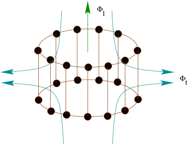
Figure 1: Schematic view of a mesoscopic cylinder subjected to both the longitudinal and transverse magnetic fluxes $\phi_{l}$ and $\phi_{t}$ respectively. Filled circles correspond to the position of the atomic sites (for color illustration, see the web version).

gives the nearest-neighbor hopping integral in the lower (upper) ring, while the parameter $v_{t}$ corresponds to the transverse hopping strength between the two rings of the cylinder. $\theta_{1}$ and $\theta_{2}$ are the two phase factors those are related to the longitudinal and transverse fluxes by the expressions, $\theta_{1}=2\pi\phi_{l}/N\phi_{0}$ and $\theta_{2}=\pi\phi_{t}/N\phi_{0}$, where $N$ represents the total number of atomic sites in each ring.

At absolute zero temperature ($T=0$ K), the longitudinal persistent current so-called the Aharonov-Bohm persistent current in the cylinder can be expressed as,

$$I(\phi_{l})=-\frac{\partial{E_{0}(\phi_{l},\phi_{t}})}{\partial{\phi_{l}}}$$ (2)

where, $E_{0}(\phi_{l},\phi_{t})$ represents the ground state energy. We evaluate this energy exactly to understand unambiguously the anomalous behavior of persistent current, and this is achieved by exact diagonalization of the tight-binding Hamiltonian Eq. (1). Throughout the calculations, we take the site energies $\epsilon_{i}^{L}=\epsilon_{i}^{U}=0$, which reveal a perfect cylinder, the hopping integrals $v_{l}^{L}=v_{l}^{U}=v_{t}=2.5$, and for simplicity, we use the units where $c=1$, $e=1$ and $h=1$.

3 Results and discussion

To reveal the basic mechanisms of the transverse magnetic flux $\phi_{t}$ on the persistent current, here we present all the results only for the non-interacting electron picture. With this assumption, the model becomes quite simple and all the basic features can be well understood. Another realistic assumption is that, we focus on the perfect cylinders only i.e., the site energies are taken as $\epsilon_{i}^{L}=\epsilon_{i}^{U}=0$ for all $i$.

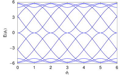
Figure 2: Variation of the energy levels as a function of the longitudinal magnetic flux $\phi_{l}$ for a mesoscopic cylinder with $N=6$. The transverse magnetic flux $\phi_{t}$ is set to $4$ (for color illustration, see the web version).

To illustrate the behavior of the persistent current in our concerned system, let us first explain the energy-flux characteristics of a mesoscopic cylinder subjected to both $\phi_{l}$ and $\phi_{t}$. Figure 2 illustrates the variation of the energy levels as a function of $\phi_{l}$ for such a mesoscopic cylinder with $N=6$. In this case, the transverse magnetic flux $\phi_{t}$ is set to $4$. The spectrum shows that the energy levels have extrema i.e., either a maxima or a minima at half-integer or integer multiples of the elementary flux-quantum $\phi_{0}$ ($=1$, for our chosen units). At these extrema points the persistent current vanishes since it is evaluated from the first derivative of the energy eigenstate with respect to the flux $\phi_{l}$ (Eq. (2)). All these energy levels vary periodically with $\phi_{l}$, showing $\phi_{0}$ flux-quantum periodicity, as expected. This $\phi_{0}$-periodicity cannot be clearly understood from the spectrum (Fig. 2) since the individual energy levels overlap with each other and form a complicated picture. The $\phi_{l}$-dependence of the energy levels and their periodicity are quite familiar to us. The significant behavior appears only when we plot the variation of the energy levels as a function of the transverse magnetic flux $\phi_{t}$. In Fig. 3, we display the dependence of the energy levels with $\phi_{t}$ for a typical mesoscopic cylinder with $N=6$. The longitudinal magnetic flux $\phi_{l}$ is fixed at $0.3$. All the energy levels get modified enormously with $\phi_{t}$, and the dependence of them also changes quite a significant way compared to the energy levels plotted in the previous spectrum (Fig. 2). The locations of the extrema points of these energy levels no longer situate at the same points as obtained in Fig. 2. In this spectrum (Fig. 3),

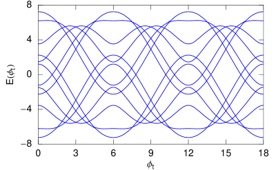
Figure 3: Variation of the energy levels as a function of the transverse magnetic flux $\phi_{t}$ for a mesoscopic cylinder with $N=6$. The longitudinal magnetic flux $\phi_{l}$ is set to $0.3$ (for color illustration, see the web version).

all the energy levels vary periodically with $\phi_{t}$, and most interestingly we observe that the energy levels exhibit $N\phi_{0}$ flux-quantum periodicity, instead of $\phi_{0}$. Since in this particular cylinder we choose $N=6$ for each ring, the energy levels provide $6\phi_{0}$ ($=6$) flux-quantum periodicity with $\phi_{t}$. The signature of this $N\phi_{0}$ periodicity becomes much more clearly visible from our study of the $I_{typ}$ vs. $\phi_{t}$ characteristics, which we shall describe at the end of this section.

Following the above discussion, next we concentrate our study on the current-flux characteristics and the dependence of the current on the transverse magnetic flux $\phi_{t}$. We evaluate all the currents only for those cylinders which contain fixed number of electrons $N_{e}$. The current carried by an energy eigenstate is obtained by taking the first order derivative of the energy for that particular state with respect to the flux $\phi_{l}$, and thus, for the $n$-th energy eigenstate of energy $E_{n}$ (say) the current can be expressed by the relation, $I_{n}(\phi_{l})=\partial E_{n}/\partial\phi_{l}$. At absolute zero temperature ($T=0$ K), the total persistent current becomes the sum of the individual contributions from the lowest $N_{e}$ energy eigenstates. The behavior of the current-flux characteristics for a impurity free mesoscopic cylinder with $N=20$ is shown in Fig. 4, where (a) and (b) correspond to the currents for $N_{e}=15$ (odd $N_{e}$) and $18$ (even $N_{e}$) respectively. The red, green and blue curves represent the results for $\phi_{t}=0$, $4$ and $10$ respectively. The current exhibits a saw-tooth

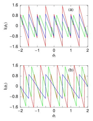
Figure 4: Persistent currents as a function of the longitudinal magnetic flux $\phi_{l}$ for a mesoscopic cylinder with $N=20$. The currents are computed for the fixed number of electrons $N_{e}$, where (a) $N_{e}=15$ and (b) $N_{e}=18$. The red, green and blue curves correspond to $\phi_{t}=0$, $4$ and $10$, respectively (for color illustration, see the web version).

like nature with sharp transitions at several points of $\phi_{l}$. This is due to the existence of the degenerate energy eigenvalues at these respective flux points. Depending on the choices of the total number of electrons $N_{e}$, the kink appears at different values of $\phi_{l}$, as expected for a multi-channel system.³⁴ All these kinks disappear as long as we introduce impurities in the system. This phenomenon is very well established in the literature and due the obvious reason we do not describe further the effect of impurities on the persistent current in the present manuscript. From a careful investigation it is observed that the current amplitude for a typical value of $\phi_{l}$ can be controlled very nicely by tuning the transverse magnetic flux $\phi_{t}$.

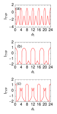
Figure 5: Typical current amplitudes as a function of the transverse magnetic flux $\phi_{t}$ for the three different mesoscopic cylinders, where (a) $N=4$, (b) $N=6$ and (c) $N=8$, respectively. The parameter $\phi_{l}$ is set to $0.25$ (for color illustration, see the web version).

Now to have a deeper insight to the effects of the transverse magnetic flux on persistent current, we focus our study on the variation of the typical current amplitude ($I_{typ}$) with the magnetic flux $\phi_{t}$. As illustrative example, in Fig. 5 we display the variation of the typical current amplitude $I_{typ}$ as a function of $\phi_{t}$, where the parameter $\phi_{l}$ is fixed to $0.25$. Figures 5(a), (b) and (c) correspond to the results for the cylinders with $N=4$, $6$ and $8$ respectively. Quite interestingly we see that the typical current amplitude varies periodically with $\phi_{t}$ providing $N\phi_{0}$ flux-quantum periodicity, instead of the conventional $\phi_{0}$ periodicity. Thus for the cylinder with $N=4$, the current exhibits $4\phi_{0}$ ($=4$) periodicity, while it becomes $6\phi_{0}$ ($=6$) for the cylinder with $N=6$ and $8\phi_{0}$ ($=8$) for the cylinder with $N=8$. From these results we clearly observe that the variation of $I_{typ}$ with $\phi_{t}$ within a period for the cylinder with $N=8$ is exactly similar to that of the cylinders with $N=6$ and $N=4$ within their single periods. Such an $N\phi_{0}$ periodicity is just the replica of the $E$ versus $\phi_{t}$ characteristics which we have described earlier. This phenomenon is really a very interesting one and may provide a new aspect of persistent current for multi-channel cylinders in the presence of the radial magnetic field $B_{r}$.

4 Concluding remarks

In conclusion, we have studied persistent currents in a mesoscopic cylinder subjected to the longitudinal magnetic flux $\phi_{l}$ and to the transverse magnetic flux $\phi_{t}$. We have used a simple tight-binding model to describe the system and calculated all the results exactly within the non-interacting electron picture. Quite interestingly we have observed that the typical current amplitude oscillates as a function of the transverse magnetic flux $\phi_{t}$, associated with the energy-flux characteristics, providing $N\phi_{0}$ flux-quantum periodicity. This phenomenon is completely different from the conventional oscillatory behavior, like as we have got for the case of $I$ versus $\phi_{l}$ characteristic which shows simple $\phi_{0}$ flux-quantum periodicity. This study may provide a new aspect of persistent current for multi-channel cylindrical systems in the presence of the radial magnetic field $B_{r}$.

This is our first step to describe how the persistent current in a thin cylinder can be controlled very nicely by means of the transverse magnetic flux. Here we have made several realistic assumptions by ignoring the effects of the electron-electron correlation, disorder, temperature, chemical potential, etc. All these effects can be incorporated quite easily with this present formalism and we need further study in such systems.

Acknowledgments

I acknowledge with deep sense of gratitude the illuminating comments and suggestions I have received from Prof. Arunava Chakrabarti and Prof. S. N. Karmakar during the calculations.

References

- [1] Y. Aharonov and D. Bohm, Phys. Rev. 115, 485 (1959).
- [2] F. Hund, Ann. Phys. (Leipzig) 32, 102 (1938).
- [3] M. Büttiker, Y. Imry, and R. Landauer, Phys. Lett. A 96, 365 (1983).
- [4] L. P. Levy, G. Dolan, J. Dunsmuir, and H Bouchiat, Phys. Rev. Lett. 64, 2074 (1990).
- [5] D. Mailly, C. Chapelier, and A. Benoit, Phys. Rev. Lett. 70, 2020 (1993).
- [6] V. Chandrasekhar, R. A. Webb, M. J. Brady, M. B. Ketchen, W. J. Gallagher, and A. Kleinsasser, Phys. Rev. Lett. 67, 3578 (1991).
- [7] E. M. Q. Jariwala, P. Mohanty, M. B. Ketchen, and R. A. Webb, Phys. Rev. Lett. 86, 1594 (2001).
- [8] N. Yu and M. Fowler, Phys. Rev. B 45, 11795 (1992).
- [9] R. Deblock, R. Bel, B. Reulet, H. Bouchiat, and D. Mailly, Phys. Rev. Lett. 89, 206803 (2002).
- [10] M. Büttiker, Phys. Rev. B 32, 1846 (1985).
- [11] H-F Cheung, E. K. Riedel, and Y. Gefen, Phys. Rev. Lett. 62, 587 (1989).
- [12] H. F. Cheung, Y. Gefen, E. K. Riedel, and W. H. Shih, Phys. Rev. B 37, 6050 (1988).
- [13] R. Landauer and M. Büttiker, Phys. Rev. Lett. 54, 2049 (1985).
- [14] N. Byers and C. N. Yang, Phys. Rev. Lett. 7, 46 (1961).
- [15] F. von Oppen and E. K. Riedel, Phys. Rev. Lett. 66, 84 (1991).
- [16] G. Montambaux, H. Bouchiat, D. Sigeti, and R. Friesner, Phys. Rev. B 42, 7647 (1990).
- [17] H. Bouchiat and G. Montambaux, J. Phys. (Paris) 50, 2695 (1989).
- [18] B. L. Altshuler, Y. Gefen, and Y. Imry, Phys. Rev. Lett. 66, 88 (1991).
- [19] A. Schmid, Phys. Rev. Lett. 66, 80 (1991).
- [20] S. K. Maiti, Int. J. Mod. Phys. B 22, 4951 (2008).
- [21] M. Abraham and R. Berkovits, Phys. Rev. Lett. 70, 1509 (1993).
- [22] A. Müller-Groeling and H. A. Weidenmuller, Phys. Rev. B 49, 4752 (1994).
- [23] I. O. Kulik, Physica B 284, 1880 (2000).
- [24] P. A. Orellana, M. L. Ladron de Guevara, M. Pacheco, and A. Latge, Phys. Rev. B 68, 195321 (2003).
- [25] I. O. Kulik, JETP Lett. 11, 275 (1970).
- [26] S. K. Maiti, J. Chowdhury, and S. N. Karmakar, Solid State Commun. 135, 278 (2005).
- [27] S. K. Maiti, J. Chowdhury, and S. N. Karmakar, Synthetic Metals 155, 430 (2005).
- [28] S. K. Maiti, Int. J. Mod. Phys. B 21, 179 (2007).
- [29] S. K. Maiti, J. Chowdhury, and S. N. Karmakar, J. Phys.: Condens Matter 18, 5349 (2006).
- [30] K. Yakubo, Y. Avishai, and D. Cohen, Phys. Rev. B 67, 125319 (2003).
- [31] E. H. M. Ferreira, M. C. Nemes, M. D. Sampaio, and H. A. Weidenmüller, Phys. Lett. A 333, 146 (2004).
- [32] S. K. Maiti, Int. J. Mod. Phys. B 21, 3001 (2007); [Addendum: Int. J. Mod. Phys. B 22, 2197 (2008)].
- [33] S. K. Maiti, Phy. Scr. 73, 519 (2006); [Addendum: Phy. Scr. 78, 019801 (2008)].
- [34] S. K. Maiti, Physica E 31, 117 (2006).