A numerical model of the VKS experiment

Abstract

We present numerical simulations of the magnetic field generated by the flow of liquid sodium driven by two counter-rotating impellers (VKS experiment). Using a kinematic code in cylindrical geometry, it is shown that different magnetic modes can be generated depending on the flow configuration. While the time averaged axisymmetric mean flow generates an equatorial dipole, our simulations show that an axial field of either dipolar or quadrupolar symmetry can be generated by taking into account non-axisymmetric components of the flow. Moreover, we show that by breaking a symmetry of the flow, the magnetic field becomes oscillatory. This leads to reversals of the axial dipole polarity, involving a competition with the quadrupolar component.

1 Introduction

The dynamo effect is a process by which a magnetic field is generated by the flow of an electrically conducting fluid. It is believed to be responsible for magnetic fields of planets, stars and galaxies [1]. Fluid dynamos have been observed in laboratory experiments in Karlsruhe [2] and Riga [3]. More recently, the VKS experiment displayed self-generation in a less constrained geometry, i.e., a von Kármán swirling flow generated between two counter-rotating disks in a cylinder [4]. In contrast with Karlsruhe and Riga experiments, the observed magnetic field strongly differs from the one computed taking into account the mean flow alone. Previous simulations, using the mean flow (time averaged) of the VKS experiment or an analytical velocity field with the same geometry, predicted an equatorial dipole [5, 6, 7, 8] in contradiction with the axial dipole observed in the experiment. Understanding the geometry of the magnetic field observed in the experiment is still an open problem. In addition, time-dependent regimes, including field reversals are observed when the impellers rotate at different frequencies [9]. No numerical study of this effect have been performed so far. We address these problems using a kinematic dynamo code in a cylindrical geometry. By considering time dependent and non-axisymmetric fluctuations of the velocity field, we show that the system is able to generate a nearly axisymmetric dipolar field. Another result of this study is that when the analytic flow mimics two disks counter-rotating with different frequencies, the system bifurcates to a regime of oscillations between dipole and quadrupole, illustrating a recent model proposed in [10] in order to explain reversals of the magnetic field in the VKS experiment or in the Earth. We will see that an $\alpha-\omega$ mechanism can explain the generation of the axial field and we understand the transition to oscillations as a saddle node bifurcation associated with the breaking of a symmetry in the flow.

2 Numerical model

In the VKS experiment, a turbulent von Kármán flow of liquid sodium is generated by two counter-rotating impellers (with rotation frequencies $F_{1}$ and $F_{2}$). The impellers are made of iron disks of radius $154$ mm, fitted with $8$ iron blades of height $41.2$ mm, and are placed $371$ mm apart in an inner cylinder of radius $206$ mm and length $524$ mm. It is surrounded by sodium at rest in another concentric cylindrical vessel, $578$ mm in inner diameter. The magnetic Reynolds numbers are defined as $R_{mi}=2\pi\mu_{0}\sigma R^{2}F_{i}$ where $\mu_{0}$ is the magnetic permeability of vacuum. When the impellers are operated at equal and opposite rotation rates $F$, a statistically stationary magnetic field with either polarity is generated above $R_{m}\sim 30$ [4]. The mean field involves an azimuthal component and a poloidal one which is dominated by an axial dipole.

When the disks are counter-rotating at the same frequency, the structure of the mean flow (averaged in time) has the following characteristics: the fluid is ejected radially from the disks by centrifugal force and loops back towards the axis in the mid-plane between the impellers. A strong differential rotation is superimposed on this poloidal flow, which generates a high shear in the mid-plane. Because of the axisymmetry of this flow, we expect from Cowling’s theorem that an axisymmetric magnetic field can not be generated. Simulations based on the mean flow indeed generate a non-axisymmetric equatorial dipole [5, 6, 7]. A better description of the VKS experiment clearly needs to involve the non-axisymmetric components of the flow. In this perspective, the geometry of the experimentally observed field has been understood with a simple model of an $\alpha-\omega$ dynamo [11]. In the VKS experiment, the strong differential rotation is very efficient to convert poloidal into toroidal magnetic field, via an $\omega$ effect. In addition, the flow that is ejected by the centrifugal force close to each impeller is strongly helical due to the vortices created between the successive $8$ blades. This non-axisymmetric helical flow drives an $\alpha$ effect which converts the toroidal field in a poloidal one. These two effects have been proposed as being responsible for the magnetic field generation, which thus results from an $\alpha-\omega$ dynamo. In the present study, we consider an analytic test velocity $u$ taking into account the time dependent $m=8$ structure due to the blades as follows:

$$\mbox{\boldmath$u$}={\bf U}+\mbox{\boldmath$\nabla$}\times\left(\kappa{\mbox{\boldmath$G$}}\right),$$ (1)

where ${\bf U}$ mimics the mean flow. It is given in cylindrical coordinates $(r,\phi,z)$ by

$$U_{r} = -{\pi\over 2}r{\left(1-r\right)}^{2}\left(1+2r\right)\cos\left(\pi z\right),$$ (2)

$$U_{\phi} = {8\over\pi}r\left(1-r\right)\arcsin\left(z\right),$$ (3)

$$U_{z} = \left(1-r\right)\left(1+r-5r^{2}\right)\sin\left(\pi z\right).$$ (4)

The vector potential $G$ describes the non-axisymmetric fluctuations due to the blades of the disks. A simple way to represent these vortices is to take :

$$G_{r}=\left[1+\cos\left(m\phi-\omega_{1}t\right)\right]r\sin(\pi r)e^{-\zeta(z-1)^{2}}\left(z-1\right)\\ +\left[1+\cos\left(m\phi+\omega_{2}t\right)\right]r\sin(\pi r)e^{-\zeta(z+1)^{2}}\left(z+1\right),$$ (5)

$$G_{\phi}=-{3}r^{2}{\left(1-r\right)}^{2}\left(1+2r\right)z^{2}\sin\left(\pi z\right)\cos(m\phi\pm\omega_{i}t).$$ (6)

In this expression, $G_{r}$ is related to a flow in the ($z,\phi$) plane and models the $8$ vortices created by the blades of each disk. These vortices are rotating with the two disks at angular velocity $\omega_{1}$ and $\omega_{2}$. The $G_{\phi}$ function represents the $\phi$-modulation of the poloidal mean recirculation associated with these vortices. The $z$ dependence of $G_{r}$ is parametrized by $\zeta$ and determines the extension of the perturbation close to the disks. The relative intensity of the mean flow and the non-axisymmetric perturbation is fixed by the value of $\kappa$. Note that the system presents an important symmetry: the flow is invariant by a rotation of an angle $\pi$ around any axis in the equatorial plane. In the following, we will denote this symmetry by $R_{\pi}$. In some simulations, we will describe the situation where one of the disks is spinning faster than the other one, thus breaking the $R_{\pi}$ symmetry. As in the symmetric case, there are several ways to implement this situation in our analytical velocity, and we take the simplest one. Spinning one disks faster than the other one is simulated by adding a global rotation ${\bf W}$ with recirculation which breaks the $R_{\pi}$ symmetry. In this case, ${\bf U}$ become ${\bf U}+C{\bf W}$, with ${\bf W}$ defined by

$$W_{r} = {\pi\over 4}r{\left(1-r\right)}^{2}\left(1+2r\right)\sin\left(\pi z/2\right),$$ (7)

$$W_{\phi} = 6r\left(1-r\right),$$ (8)

$$W_{z} = \left(1-r\right)\left(1+r-5r^{2}\right)\cos\left(\pi z/2\right).$$ (9)

This is the mean flow corresponding to the disk at $z=+1$ spinning alone. The parameter $C$ thus controls the deviation from exact counter-rotation ($C=0$), and traces back to the difference between the two disk frequencies in the VKS experiment. In addition, it is reasonnable to assume that the non-axisymetric velocity component is also modified when $C\neq 0$. This is achieved by the simple transformation $\omega_{1}=\omega_{1}(1+C)$ and $\kappa=\kappa(1+C)$ for $z>0$.

Note that the expression for the velocity used here is arbitrary, and there are probably several ways to describe with more accuracy the von Karman flow. However, the purpose of this study is to show that the structure and the dynamics of the magnetic field in the VKS experiment can be easily reproduced by taking into account the main geometrical properties of the flow, i.e. the vortical structure near the disks and the breaking of the $R_{\pi}$ symmetry when the disks counter-rotate at different frequencies.

We perform direct numerical simulations of the kinematic dynamo problem, solving the induction equation governing the evolution of the solenoidal magnetic field $\bf B$

$$\frac{\partial\mbox{\boldmath$B$}}{\partial t}=\mbox{\boldmath$\nabla$}\times\left(\mbox{\boldmath$u$}\times\mbox{\boldmath$B$}\right)+\frac{1}{Rm}\Delta\mbox{\boldmath$B$}\,,$$ (10)

written in dimensionless form using the advective timescale. The magnetic Reynolds number $Rm$ is defined as $Rm=\mu_{0}\sigma RU_{max}$, where $R$ is the radius of the impellers and $U_{max}$ is the peak velocity of the mean flow. The radius of the cylinder is $L=4R/3$ and the total height is $H=2L$.

The above system with the flow given in (1) is solved using a finite volume code adapted from [12]. A filtering of high-frequency modes in the $\phi$ direction has been implemented to circumvent the severe restriction on the CFL number induced by cylindrical coordinates near the axis. Also a centered second order scheme has been prefered to an up-wind scheme as resistive effects are here important enough to regularise the solution. As in [12], we ensure that $\mbox{\boldmath$\nabla$}\cdot\mbox{\boldmath$B$}=0$ is exactly satisfied using a constraint transport algorithm. The finite volume solver is fully three-dimensional. Two types of magnetic boundary conditions are used: insulating boundaries, using the boundary element formalism as introduced in [13], or ferromagnetic boundaries, by forcing the magnetic field lines to be normal to the external wall, as used in [7]. In all cases we do not include sodium at rest around the vessel or behind the disks.

3 Structure of the magnetic field

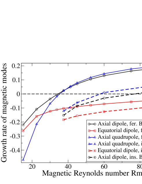
Figure 1: Evolution of the growth rates of the magnetic modes when $Rm$ is increased in exact counter-rotation. For ferromagnetic boundaries, we show the $m=0$ axial dipolar mode (circles). Triangles: $m=0$ quadrupolar field. Squares: equatorial dipole. Note the close values of the onset for dipole and quadrupole. Growth rates with insulating boundaries are also displayed (dashed lines), showing much larger onset values for all modes.

The convergence of the numerical implementation has been carefully validated comparing simulations at different resolutions. We report results obtained with a resolution of $150\times 150\times 128$ . In the simulations presented here, we use $\zeta=30$ and $\kappa=1$. This corresponds to vortices of a typical size of $1/5$ of the total height of the cylinder, and with a velocity of the same order than the mean flow. These parameters are comparable to what is expected in the real experiment. Let us study first the situation corresponding to the counter-rotating case. Figure  1 shows the growth rate of different magnetic modes as a function of the magnetic Reynolds number. We see that the non-axisymetric flow leads to the generation of an axisymmetric $m=0$ magnetic mode with a dipolar symmetry, which bifurcates for $Rm\approx 34$, using ferromagnetic boundary conditions. Because of the $m=8$ structure in the velocity field, this mode is in fact associated with a $m=8$ magnetic component, growing at the same rate. However, this small scale structure is time dependent and averages on a few advective times. In figure  1, we see that the first unstable mode is an axial dipole similar to the mean field observed in the VKS experiment, and that the quadrupolar mode is also unstable for larger $Rm$. The other modes are not unstable in the range of $Rm$ studied here. In particular, we see that the non axisymmetric component of the flow strongly inhibits the $m=1$ equatorial dipole, which bifurcates around $Rm=45$ for $\kappa=0$, i.e. with the mean flow alone (see figure 2, bottom). In general, the two first axial modes always display similar threshold values, and depending on the parameters of the flow, the first unstable axisymmetric structure can be either a dipole or a quadrupole. In the VKS experiment, a quadrupolar field has never been observed for counter-rotation of the disks at the same frequency. The different magnetic structures are represented in figure  2.

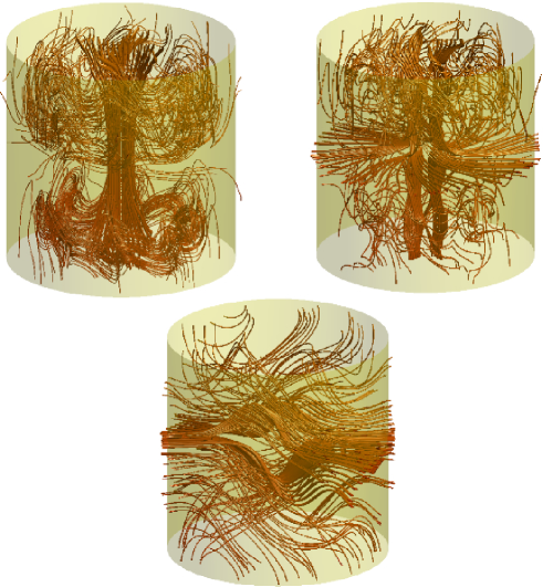
Figure 2: Snapshot of the magnetic field lines of different modes obtained in the numerical simulations. Axial dipole (top, left), quadrupolar (top, right) and equatorial dipole (bottom). Observe that the axial modes always involve $m=8$ component.

In figure 3, we represent the radial profiles of the axisymmetric components of the dipole for $Rm=36$, which are similar to the ones of the mean field observed in the VKS experiment [14]. These results confirm the mechanism proposed in [11], which states that the non-axisymmetric vortices near the disks could be responsible for the generation of the observed magnetic field. In a recent $\alpha$-parametrized mean field approach, a completely different result was found, for which the $\alpha$ term is said to be several times larger than any realistic value based on the VKS experiment [15]. Here, our study shows a critical $Rm$ comparable to the experiment. In addition, the maximum intensity of the vortices compared to the mean flow, about a factor $1.5$ here for $\kappa=1$, is reasonnable. Figure  1 also shows the effect of the magnetic boundary conditions on the dynamo threshold of the different modes. We see that using ferromagnetic boundary conditions is very efficient for decreasing the dynamo threshold. For insulating boundaries, the $m=0$ mode bifurcates for $Rm=58$, whereas its threshold is $Rm=34$ for ferromagnetic boundary conditions. Note that in the case of insulating boundaries, the first unstable mode is a quadrupole, and the axial dipole bifurcates for $Rm=76$. This confirms the role played by soft iron disks in the experiment: changing the geometry of the magnetic field lines near the external wall yields a strong reduction of the instability threshold. This was already observed with the mean flow alone [7] and could explain why dynamo action has only been observed in the VKS experiment when soft iron disks are used.

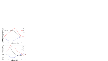
Figure 3: Comparison of the numerical simulations (top) and experimental results (bottom). We show the radial profiles for the 3 components of the axial dipolar field measured near one of the disks, when the disks counter-rotate for $Rm=36$. Fields have been $\phi$-averaged (simulations) or time averaged (experimental data, from [14]).

4 Dynamics of the magnetic field for different rotation rates

In the VKS experiment, several dynamical behaviors occur when the rotation rates of the two disks are differents: periodic oscillations, bursts and chaotic reversals of the magnetic field have been reported. When the velocity difference of the disks is increased from zero, the stationnary dipolar field is first modified by the addition of a quadrupolar component before diplaying a transition to a time dependent regime [16].

When the disks counter-rotates at the same frequency, the flow is invariant under the $R_{\pi}$ symmetry. Consequentely, dipolar and quadrupolar modes, which transform differently under $R_{\pi}$, are linearly decoupled. We observe in figure 1 that the dipole and quadrupole modes have slightly different growth rates at the dynamo onset, the neutral mode being a dipolar mode (see figure  2, bottom). When one disk is spinning faster than the other one, the $R_{\pi}$ symmetry of the flow is broken and dipolar and quadrupolar modes get coupled. Consequentely, the growing unstable mode has to be a combination of a dipole and a quadrupole. The ratio between dipolar and quadrupolar components depends on the intensity of the breaking of the $R_{\pi}$ symmetry.

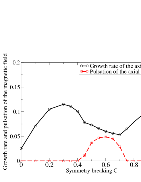
Figure 4: Evolution of the growth rate and pulsation of the axial mode when the $R_{\pi}$ symmetry is broken. For $C<0.4$, the growing mode is a combination of a dipole and a quadrupole (growth rate, black circles). At $C=0.4$ the system undergoes a bifurcation to oscillations (red squares). Note that, in this range, the oscillatory regime only occurs in a pocket of the parameter space, for $0.4<C<0.75$.

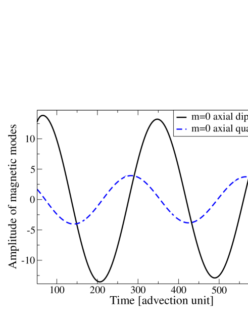
Figure 5: Time evolution of the magnetic field during oscillations. The system is very close to criticality, for $Rm=30$ and $C=0.6$, such that the growth rate is very small. Note the transfer between the axial dipole ( full line) and the quadrupole (dashed line).

Figure  4 shows the evolution of the growth rates of the modes when we increase the parameter $C$ representing the departure from counter-rotation. We start from $Rm=37$, and $C$ is increased from zero to one. Because of the breaking of the $R_{\pi}$ symmetry when $C\neq 0$, the growing mode is not a pure dipole anymore. Similarly, the initially quadrupolar mode displays some dipolar component. In this linear problem, only the most unstable mode is easily obtained from the simulations, since dipolar and quadrupolar families are mixed when the $R_{\pi}$ symmetry is broken. We see that the growth rate of the axial mode is changed when $C$ is increased. For $C=0.4$, the system bifurcates to an oscillatory regime, when two different real eigenvalues transform into complex conjugate ones. These results have been recently understood in the framework of a simple model, based on a saddle node bifurcation [10]. If we denote by $D$ the amplitude of the eigenmode with dipolar symmetry and by $Q$ the quadrupolar one, a simple way to understand these linear results is to write the evolution of the modes near the threshold:

$$\dot{D}=\alpha(C)D+\beta(C)Q,$$ (11)

$$\dot{Q}=\gamma(C)D+\delta(C)Q.$$ (12)

where dots stand for time derivation. The eigenvalues $\lambda_{i}$ of this system are given by $2\lambda_{i}=\alpha+\delta\pm\sqrt{(\alpha-\delta)^{2}+4\beta\gamma}$. When the disks are spinning at the same rotation rate, $\beta$ and $\gamma$ vanish and the dipole and the quadrupole are not linearly coupled, giving two real eingenvalues $\lambda_{1}$ and $\lambda_{2}$. For $C\neq 0$, when $\beta\gamma$ is negative and sufficiently large, $\lambda_{1}$ and $\lambda_{2}$ become complex conjugate eigenvalues. The system thus bifurcates to an oscillatory regime, in agreement with the numerical simulations shown here. The pulsation of the oscillatory mode is represented in figure 4. Note that the period of the oscillations diverges at threshold. An interesting feature is that these periodic reversals of the magnetic field only occur in a small range of the parameter space, for $0.4<C<0.75$. This shows that the relation between $C$ and the parameters of the system are rather complex. This is also the case in the VKS experiment, where reversals, periodic oscillations and bursts appear only in small pockets in the parameter space.

Figure 5 displays a typical time evolution of the magnetic field during oscillations. Here, the system is investigated very close to criticality ($Rm=30$ and $C=1.6$), such that the exponential behavior is very weak. These oscillations involve a competition between an axial dipole and an axial quadrupole. We see in particular that the two components are in quadrature. This means that the magnetic field does change shape. The present study being linear, it can only illustrate the transition between stationnary and oscillatory dynamos. In particular, the present simulations cannot reproduce the non-periodic reversals of the magnetic field observed in the VKS experiment [9]. This more realistic situation is reported in [17], where chaotic reversals of the magnetic field are observed in fully turbulent simulations.

5 Conclusion

In this study, we have used a simple model of a von Karman flow to describe the structure and some of the dynamical behaviors of the magnetic field in the VKS experiment. In particular, we have shown that taking into account the non-axisymmetric fluctuations of the flow leads to the generation of a nearly axisymmetric dipole. This confirms that the helical flow created by the vortices between the blades of each disk can be involved in the dynamo process, possibly via an $\alpha-\omega$ mechanism. This flow generates an axial dipole or quadrupole, and also inhibits the equatorial dipole. In addition, we have shown that the presence of ferromagnetic boundaries can strongly reduce the threshold of the dynamo instability. Another result of this study concerns the dynamics of the magnetic field. When the disks are spinning at different rates, the $R_{\pi}$ symmetry of the flow is broken. Our simulations show that this can lead to an oscillatory regime between a dipole and a quadrupole, similar to the one observed in the VKS experiment. The agreement between the experimental results and these numerical simulations show that, despite the high level of turbulence and complexity of the flow, the generation of the magnetic field can be understood using a few spatial properties of the flow. Moreover, the mechanisms involved in the dynamics of the field can be accurately described with a low dimensional model.