Zero Sound in Dipolar Fermi Gases

Abstract

We study the propagation of sound in a homogeneous dipolar gas at zero temperature, known as zero sound. We find that undamped sound propagation is possible only in a range of solid angles around the direction of polarization of the dipoles. Above a critical dipole moment, we find an unstable mode, by which the gas collapses locally perpendicular to the dipoles’ direction.

I Introduction

At ultracold temperatures, the usual propagation of thermodynamic sound waves in a gas is suppressed due to the rarity of collisions. Nevertheless, in a Fermi gas, collective excitations known as zero sound can still propagate even at zero temperature Landau57 ; LLSP2 . These excitations involve a deformation of the Fermi surface in a way distinguished from that of ordinary sound. The theory of zero sound has been applied in the past to isotropic, two component Fermi liquids. Depending on the properties and strength of the interaction,one observes the possibility of different propagation modes (longitudinal or transverse) as well as the possibility of no zero sound propagation at all. Zero sound has been measured experimentally in liquid He-3 Abel66 ; Roach76 in which both longitudinal and transverse modes of zero sound co-exist. Another type of collective excitations that exist for two component Fermi liquids is spin-dependent vibrations known as spin waves.

Here we shall be interested in zero sound in a homogeneous, single component dipolar Fermi gas, where all the dipoles are oriented in one direction by an external field. In particular we are interested in the question of how zero sound propagation is affected by the long range and anisotropic nature of the dipolar interaction. In the case of Bose-Einstein condensates (BEC’s), strong dipolar effects have been observed in a gas of Chromium-52 atoms with relatively big magnetic moments Lahaye07 ; Koch08 ; Lahaye08 - for a recent review of dipolar BEC’s see Lahaye09 . In the case of Fermi gases, the atomic magnetic dipolar interaction is small compared to the Fermi energy, so it may be hard to observe dipolar effects. However much stronger effects are expected in an ultracold gas of hetronuclear molecules with electric dipoles, where the dipolar interaction is considerably larger (such an ultracold gas of fermionic KRb molecules has been recently realized in experiment Ospelkaus08a ; Ni08 ). Previous theoretical work on ultracold dipolar Fermi gases studied their ground state properties and expansion dynamics in the normal phase Goral01 ; Miyakawa08 ; Sogo08 ; Fregoso09 , as well as BCS superfluidity Baranov02b ; Baranov04 . It has been shown that both the critical temperature for the superfluid transition, and the BCS order parameter, are sensitive to the aspect ratio of the trap. In the case of a cigar trap, the order parameter becomes non-monotonic as a function of distance from the center of the trap, and even switches sign. However, zero sound refers to phenomena in the normal phase, therefore we are interested in the regime of temperatures which are well below the Fermi temperature $T_{F}$, but still above the critical BCS temperature. Zero sound in Fermi dilute gases of alkali type (with contact interactions), in the crossover from 3D to 2D, has been recently studied in Ref. Mazzarella09 .

An interesting result due to Miyakawa eta al. (Miyakawa08 , Sogo08 ) is that the Fermi surface of a dipolar gas is deformed. They postulated an ellipsoidal variational ansatz for the Fermi surface, and by minimizing the total energy of the system, found that that it is deformed into a prolate ellipsoid in the direction of the polarization of the dipoles. As a preliminary to studying zero sound, one of our aims in the present work is to compute numerically the equilibrium Fermi surface, and thus, along the way, also check the reliability of the variational method.

This paper is organized as follows. In section (II) we find numerically the shape of the Fermi surface of a dipolar Fermi gas at equilibrium, and compare it with the variational method. In section  (III) we study the zero sound in this gas, and how it depends on the direction of propagation and the strength of the interaction. We also find the instability of the gas above a critical dipolar interaction strength, manifested in the appearance of a complex eigenfrequency. Finally we present our conclusions in section (IV).

II Shape of the Fermi surface

We consider a homogeneous, single component, dipolar gas of fermions with mass $m$ and magnetic or electric dipole moment $d$. The dipoles are assumed to be polarized along the $z$-axis. It is significant that dipolar fermions continue to interact in the zero-temperature limit, even if they are in identical internal states. This is a consequence of the long-range dipolar interaction. The system is described by the Hamiltonian:

$$H=\sum_{i=1}^{N}-\frac{\hbar^{2}}{2m}\nabla_{i}^{2}+\sum_{i\neq j}V_{dd}(\bm{r}_{i}-\bm{r}_{j}),$$ (1)

where $V_{dd}(\bm{r})=(d^{2}/r^{3})(1-3z^{2}/r^{2})$ is the two-body dipolar interaction. We use the semi-classical approach in which the one-body density matrix is given by Miyakawa08

$$\rho(r,r^{\prime})=\int\frac{d^{3}k}{(2\pi)^{3}}f\left(\frac{\bm{r}+\bm{r^{\prime}}}{2},\bm{k}\right)e^{i\bm{k}\cdot(\bm{r}-\bm{r^{\prime}})},$$ (2)

where $f(\bm{r},\bm{k})$ is the Wigner distribution function. The number density distributions in real and momentum space are given by

$$n(\bm{r})=\rho(\bm{r},\bm{r})=\int\frac{d^{3}k}{(2\pi)^{3}}f(\bm{r},\bm{k})$$ (3)

$$\tilde{n}(\bm{k})=(2\pi)^{-3}\int d^{3}rf(\bm{r},\bm{k}).$$

Within the Thomas Fermi-Dirac approximation, the total energy of the system is given by $E=E_{kin}+E_{d}+E_{ex}$, the sum of kinetic, dipolar and exchange energies, where:

$$E_{kin}=\int\frac{d^{3}k}{(2\pi)^{3}}\frac{\hbar^{2}k^{2}}{2m}f(\bm{r},\bm{k}),$$ (4)

$$E_{d}=\frac{1}{2}\int d^{3}r\int d^{3}r^{\prime}V_{dd}(\bm{r}-\bm{r^{\prime}})n(\bm{r})n(\bm{r}^{\prime}),$$ (5)

$$E_{ex} = -\frac{1}{2}\int d^{3}r\int d^{3}r^{\prime}\int\frac{d^{3}k}{(2\pi)^{3}}\int\frac{d^{3}k^{\prime}}{(2\pi)^{3}}V_{dd}(\bm{r-r^{\prime}})e^{i(\bm{k}-\bm{k^{\prime}})\cdot(\bm{r}-\bm{r^{\prime}})}\times$$

$$f\left(\frac{\bm{r}+\bm{r^{\prime}}}{2},\bm{k}\right)f\left(\frac{\bm{r+r^{\prime}}}{2},\bm{k^{\prime}}\right).$$

We shall consider a homogeneous system of volume $V$ with number density $n_{f}$. Let $k_{F}$ be the Fermi wave number of an ideal Fermi gas with that density. Then $n_{f}$ is related to $k_{F}$ by $n_{f}=k_{F}^{3}/(6\pi^{2})$. For an homogeneous gas the exchange energy can be rewritten as

$$E_{ex}=-V/2\int\frac{d^{3}k}{(2\pi)^{3}}\int\frac{d^{3}k^{\prime}}{(2\pi)^{3}}f(\bm{k})f(\bm{k^{\prime}})\tilde{V}_{dd}(\bm{k}-\bm{k^{\prime}}),$$ (7)

Here we have used the Fourier transform of the dipolar potential, $\tilde{V}_{dd}(\bm{q})=(4\pi/3)d^{2}(3\cos^{2}\theta_{\bm{q}}-1)$ where $\theta_{\bm{q}}$ is the angle between the momentum $\bm{q}$ and the direction of polarization, which is chosen to be along the $k_{z}$-axis.

For a homogeneous gas, the distribution function $f$ is a function of $\bm{k}$ only. For an ideal gas or for a gas with isotropic interactions at zero temperature, it is given by $f(\bm{k})=\Theta(k_{F}-k)$, where $\Theta(k)$ is Heaviside’s step function. This describes a Fermi sphere with radius $k_{F}$. In the case of dipolar gas, Miyakawa et al.(Miyakawa08 , sSogo08 ) postulated the following variational ansatz:

$$f(\bm{k})=\Theta\left(k_{F}^{2}-\frac{1}{\beta}(k_{x}^{2}+k_{y}^{2})-\beta^{2}k_{z}^{2}\right),$$ (8)

It is then possible to determine variationally the parameter $\beta$ that minimizes the total energy of the system. In general it is found that $\beta<1$, namely the Fermi surface is deformed into a prolate spheroid. This occurs due to the exchange interaction (Eq. (7)) being negative along the direction of polarization.

We shall first be interested here in finding the accuracy of this variational method, and also derive some analytical results for the exchange energy, in a similar fashion to the well known exchange energy of a homogeneous electron gas.

Instead of directly minimizing the total energy, our starting point is that the quasi-particle energy $\epsilon(\bm{k})\equiv\frac{(2\pi)^{3}}{V}\frac{\delta E[f]}{\delta f}$ on the Fermi surface (i.e, the chemical potential) must be constant in equilibrium. The quasi-particle energy is given by:

$$\epsilon(\bm{k})=\frac{\hbar^{2}k^{2}}{2m}-\int\frac{d^{3}k^{\prime}}{(2\pi)^{3}}f(\bm{k^{\prime}})\tilde{V}_{dd}(\bm{k}-\bm{k^{\prime}}).$$ (9)

Further we shall assume that $f(\bm{k})$ is either 0 or 1, that is, there is a well defined and sharp Fermi surface. Our first calculation is perturbative. For small $d$, the solution of $\epsilon(\bm{k})=$constant, is found. Let $\bm{\hat{n}}$ be a unit direction vector in k-space. Let $\bm{k}=k\bm{\hat{n}}$ lie on the (deformed) Fermi surface. Then we have:

$$\bm{k}=\bm{\hat{n}}\left(k_{F}+\frac{m}{k_{F}\hbar^{2}}\int\frac{d^{3}k^{\prime}}{(2\pi)^{3}}f(\bm{k^{\prime}})\tilde{V}_{dd}(k_{F}\bm{\hat{n}}-\bm{k^{\prime}})\right),$$ (10)

where, for weak interaction, $f$ on the right side can be taken to be the distribution function of an ideal gas. The integral can be evaluated analytically by using the convolution theorem, with the result:

$$k(\theta)=k_{F}+\frac{1}{9\pi}\frac{md^{2}k_{F}^{2}}{\hbar^{2}}\left(3\cos^{2}(\theta)-1\right),$$ (11)

where $\theta$ is the angle between $\bm{\hat{n}}$ and the $z$-axis. For small $d$, Eq. (11) is consistent with a Fermi surface of slightly ellipsoidal shape, Eq. (8), with $\beta=1-\frac{2}{9\pi}\frac{md^{2}k_{F}}{\hbar^{2}}$. This confirms that the ellipsoidal ansatz is indeed correct for small $d$. The corresponding energy is then

$$E/V=\frac{\hbar^{2}k_{F}^{5}}{m}\left(\frac{1}{20\pi^{2}}-\frac{1}{405\pi^{4}}(\frac{md^{2}k_{F}}{\hbar^{2}})^{2}\right),$$ (12)

and the chemical potential is

$$\mu=\frac{\hbar^{2}k_{F}^{2}}{2m}\left(1-\frac{28}{405\pi^{2}}(\frac{md^{2}k_{F}}{\hbar^{2}})^{2}\right).$$ (13)

Next, for arbitrary $d$, we solve numerically for $\epsilon(\bm{k})=$constant. The calculation is a self consistent iterative generalization of the perturbative calculation above, where the constant is adjusted to obtain a fixed number of particles.

It is convenient to present our results in terms of a dimensionless parameter

$$D\equiv\frac{md^{2}}{\hbar^{2}}k_{F},$$ (14)

which signifies the strength of the dipolar interaction between two particles separated by a distance $1/k_{F}$, in units of the Fermi energy. This dimensionless expression appears in the equations for $E/V$ and $\mu$ above. For reference, a gas density of $10^{12}$ cm^-3 with dipole moment of 1 Debye, and atomic mass of 100 amu, has D=5.8. In Fig. (1) we compare the Fermi surface found numerically with the variational Fermi surface for a strongly interacting dipolar gas with $D=12.0$. We see that even for this relatively strong interaction, the variational method works quite well. The actual Fermi surface is not exactly an ellipsoid and is slightly less prolate.

In Fig. (2a) we compare the exact and variational results for the aspect ratio of the Fermi surface shape, and in Fig. (2b) we compare the chemical potentials. For both quantities the variational method generally works very well.

Since our numerical results are close to those obtained by the variational method, we might also expect an instability, due to the inverse compressibility becoming negative, to occur around $D\approx 12.5$, as found in Ref. Sogo08 . However, a cautionary note is in place, since for such strong interactions one can expect deviations from the mean field theory, which might stabilize the gas - as occurs in the case of a two-component Fermi gas with negative contact interactions Giorgini08 .

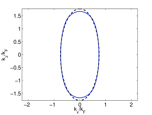
Figure 1: Shape of the Fermi surface of a homogeneous dipolar gas with interaction strength $D=12.0$. Solid line: numerical calculation. Dashed line: variational method

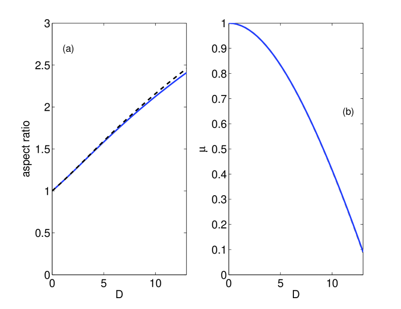
Figure 2: a) Aspect ratio of the Fermi surface of dipolar gas as a function of the interaction strength $D$. Solid line: numerical calculation. Dashed line: variational method. b) Chemical potential of dipolar gas as a function of the interaction strength $D$. $\mu$ is given in units of $\hbar^{2}k_{F}^{2}/m$. The numerical (solid) and variational (dashed) curves are virtually indistinguishable.

Recently, it has been suggested Fregoso09 that for strong enough dipolar interactions, bi-axial nematic phase should appear. Namely, above a critical interaction strength, the Fermi surface will distort into an ellipsoid with three different semi-axis, spontaneously breaking cylindrical symmetry. In our work, we assumed from the start that cylindrical symmetry of the equilibrium state is not broken, However, the bi-axial phase was predicted to occur around $D\approx 30$, which is above the compressional instability limit of $D=9.5$. In what follows, we shall restrict ourselves to discuss zero sound for $D<9.5$. In fact, we find below that the gas becomes unstable and collapses even below this limit.

III Zero Sound

We now consider collective excitations of a homogeneous dipolar Fermi gas at zero temperature, i.e zero sound. The normal speed of thermodynamic sound (first sound) is $c^{2}=\frac{1}{m}\frac{\partial P}{\partial n}$ where $P=-\frac{\partial E}{\partial V}$ is the pressure. However, thermodynamic sound is highly attenuated for a rarefied gas at low temperatures (in the collisionless regime). The attenuation of sound is due to transfer of energy from the sound wave to random molecular motion (heat), and depends on the ratio of the collision rate to the sound frequency. Specifically, the collisionless regime is obtained for $\omega\tau>>1$, where $\tau$ is the mean time between collisions, and $\omega$ the frequency of sound. In particular, for a Fermi gas, the collisionless regime is rapidly obtained when the temperature drops below the Fermi temperature, and collisions are quenched by Fermi statistics. However Landau Landau57 discovered that a collective excitation of a Fermi gas at zero temperature is still possible in this case. This zero sound is essentially a propagation of a deformation of the Fermi surface. The theory of zero sound as applied to a two component Fermi gas with short range interactions is described in standard textbooks, e.g LLSP2 ; QMPS .

Our goal is to apply this theory to the case of the one component dipolar gas. The local quasi-particle energy at position $\bm{r}$ is given by

$$\epsilon(\bm{r},\bm{k}) \equiv \frac{(2\pi)^{3}}{V}\frac{\delta E}{\delta f(\bm{r},\bm{k})}=$$

$$=\frac{\hbar^{2}k^{2}}{2m}+\int d^{3}r^{\prime}\frac{d^{3}k^{\prime}}{(2\pi)^{3}}V_{dd}(\bm{r}-\bm{r^{\prime}})f(\bm{r^{\prime}},\bm{k^{\prime}})-\int\frac{d^{3}k^{\prime}}{(2\pi)^{3}}f(\bm{r},\bm{k^{\prime}})\tilde{V}_{dd}(\bm{k^{\prime}}-\bm{k}),$$

where the last term, the contribution of exchange interaction, has been calculated within local density approximation (as in Eq. (9)), suitable for collective excitations with long wavelength. Note that, compared to Eq. (9), Eq. (III) shows an extra direct-interaction term involving $V_{dd}(\bm{r}-\bm{r^{\prime}})$. For a spatially homogeneous distribution function this term vanishes, because the angular average of the dipolar interaction is zero.

We apply a Boltzmann transport equation which reads:

$$\frac{df}{dt}\equiv\frac{\partial f}{\partial t}+\frac{1}{\hbar}\nabla_{\bm{r}}f\cdot\nabla_{\bm{k}}\epsilon-\frac{1}{\hbar}\nabla_{\bm{k}}f\cdot\nabla_{\bm{r}}\epsilon=I(f),$$ (16)

where $I(f)$ is the collision integral, and $\epsilon$ can be taken, to first order, to be the equilibrium quasi-particle energy. The collisional integral can be neglected in the collisionless regime we are interested in here. However, more generally, it is interesting to note that the dipolar interaction is long range, giving rise to both a mean field interaction ($V_{dd}(\bm{r}-\bm{r^{\prime}})$ term in the right side of Eq. (III)) and a collisional cross section that enters $I(f)$. In this respect the dynamics of dipolar Fermi gas are an intermediate between, on the one hand, plasma dynamics which to a first approximation are controlled by the mean field potential (as in Vlasov equation), and on the other hand, the dynamics of Fermi liquids with short range interactions, which are controlled by the local exchange interaction and the collisional integral.

For small deviations from equilibrium, the distribution function changes in the near vicinity of the equilibrium Fermi Surface, and can be written in the form

$$f=f_{e}+e^{i(\bm{q}\cdot\bm{r}-\omega t)}\nu(\bm{k})\delta(\epsilon_{e}(\bm{k})-\mu),$$ (17)

where $\mu$ is the equilibrium chemical potential, and $\epsilon_{e}$ is as in Eq. (9). $\nu(\bm{k})$ is a function defined on the equilibrium Fermi Surface, and will signify the eigenmode of the zero sound wave. This perturbation describes a mode with spatial wavenumber $\bm{q}$ and frequency $\omega$.

Eqs. (16) and (III) then give:

$$\left(\omega-\bm{v}(\bm{k})\cdot\bm{q}\right)\nu(\bm{k})=-\bm{v}(\bm{k})\cdot\bm{q}\oint dS^{\prime}\frac{\tilde{V}_{dd}(\bm{k}-\bm{k^{\prime}})\nu(\bm{k^{\prime}})}{(2\pi)^{3}\hbar|\bm{v}(\bm{k^{\prime}})|}+$$ (18)

$$+\bm{v}(\bm{k})\cdot\bm{q}\tilde{V}_{dd}(\bm{q})\oint dS^{\prime}\frac{\nu(\bm{k^{\prime}})}{(2\pi)^{3}\hbar|\bm{v}(\bm{k^{\prime}})|}.$$

where $\bm{v}(\bm{k})\equiv\frac{\nabla_{\bm{k}}\epsilon_{e}}{\hbar}$. In the above equation, $\bm{k}$ and $\bm{k^{\prime}}$ lie on the equilibrium Fermi surface. Also the integrals are taken on this surface. The first integral is an exchange interaction term, and the second a direct term. They can be combined to obtain:

$$\left(\omega-\bm{v}(\bm{k})\cdot\bm{q}\right)\nu(\bm{k})=\bm{v}(\bm{k})\cdot\bm{q}\oint dS^{\prime}\frac{\left(\tilde{V}_{dd}(\bm{q})-\tilde{V}_{dd}(\bm{k}-\bm{k^{\prime}})\right)\nu(\bm{k^{\prime}})}{(2\pi)^{3}\hbar|\bm{v}(\bm{k^{\prime}})|}.$$ (19)

The problem of zero sound of a dipolar gas is thus reduced to finding, for a given wavenumber $\bm{q}$, the eigenvalues $\omega$ and eigenmodes $\nu(\bm{k})$. In fact, it can be seen from Eq. (19) that $\omega$ is linear in $|\bm{q}|$, and thus we expect a linear phonon spectrum with a speed of sound which in general depends on the relative direction of the propagation direction $\bm{q}$ with respect to the direction of polarization. It can be seen that for undamped vibrations, the speed of sound $s(\hat{\bm{q}})=\frac{\omega}{|\bm{q}|}$ must exceed a critical velocity $v_{\mathrm{damp}}(\hat{\bm{q}})\equiv\max_{\bm{k}}\{\bm{v}(\bm{k})\cdot\hat{\bm{q}}\}$, where $\hat{\bm{q}}=\bm{q}/|\bm{q}|$. To see this, replace $\nu$ by another unknown function $\tilde{\nu}(\bm{k})=(\omega-\bm{v}({\bm{k}})\cdot\bm{q})\nu(\bm{k})$. Then Eq. (19) can be rewritten as:

$$\tilde{\nu}(\bm{k})=\bm{v}(\bm{k})\cdot\bm{q}\oint dS^{\prime}\frac{\left(\tilde{V}_{dd}(\bm{q})-\tilde{V}_{dd}(\bm{k}-\bm{k^{\prime}})\right)\tilde{\nu}(\bm{k^{\prime}})}{(\omega-\bm{v}(\bm{k^{\prime}})\cdot\bm{q})(2\pi)^{3}\hbar|\bm{v}(\bm{k^{\prime}})|}$$ (20)

When $\omega<\max_{\bm{k}}\{\bm{v}(\bm{k})\cdot\bm{q}\}$, the integrand has a pole, which must be avoided by going around it in the complex plane, giving an imaginary part which signifies the decay of such a vibrational mode.

Eq. (19) can be solved numerically by discretizing it on the Fermi surface. We use an evenly spaced, 64x64 grid, in spherical coordinates $\theta,\phi$, where the ’north pole’ is in the direction of polarization of the dipoles. In accordance with the discussion above, we select the undamped modes which satisfy $s(\hat{\bm{q})}>v_{\mathrm{damp}}(\hat{\bm{q}})$. For that purpose, it is sufficient to look for a few eigenmodes with the largest eigenvalues, using an Arnoldi method. We checked our numerical code by calculating the modes for the case of an isotropic Fermi Fluid LLSP2 , and comparing to the known analytic solutions.

Before discussing our results for the dipolar gas, it will be helpful to briefly review the known results for two component isotropic Fermi liquids. The case relevant to us is that of same spin vibrations, in which the two components move in unison. For an isotropic fluid the Fermi surface is a sphere. The interaction term

$$F(\bm{q},\bm{k},\bm{k^{\prime}})\equiv\tilde{V}_{dd}(\bm{q})-\tilde{V}_{dd}(\bm{k}-\bm{k^{\prime}}),$$ (21)

which appears in Eq.(19), is replaced, in the case of isotropic liquids, by $F(\bm{k},\bm{k^{\prime}})=\frac{2\pi^{2}\hbar}{mk_{F}}\left(F_{0}+F_{1}\bm{\hat{k}}\cdot\bm{\hat{k}^{\prime}}\right)$, where $F_{0}$ and $F_{1}$ are the Landau parameters. One finds the following. When $F_{1}=0$ and $F_{0}>0$ there is a longitudinal mode which is concentrated on the Fermi sphere around the forward direction of propagation, which becomes more and more concentrated around that point as $F_{0}\rightarrow 0$. For $F_{1}=0$ and $F_{0}<0$, no zero sound propagation exists. For $F_{1}>6$, there also exists a transverse mode which has a vortex like structure on the Fermi surface around the direction of propagation.

We now examine the results for the dipolar gas. Fig. (3) shows the speed of sound $s=\omega/q$ in the dipolar Fermi gas for interaction strength parameter $D=1$, as a function of the angle $\alpha$ between the direction of sound propagation and the direction of polarization. We find one zero sound mode which, for small $\alpha$, satisfies the criterion for propagation However sound does not propagate in all directions: for $\alpha>\alpha_{c}\approx 0.6$ the gap between the calculated speed of sound and the propagation limit $v_{\mathrm{damp}}$ is essentially zero. This means that there is no undamped propagating zero sound for a wide range of angles around the direction perpendicular to the direction of polarization.

To understand this result, we borrow lessons learned from the case of isotropic Fermi fluids. There, we know that spin-independent, longitudinal zero sound mode, only propagates for repulsive interaction (positive landau parameter $F_{0}$), and is damped for attractive interaction (negative landau parameter $F_{0}$). Thus, it makes sense that the anisotropy of the dipolar interaction gives rise to sound propagation only in a certain range of directions around the direction of polarization, where the effective interaction in momentum space is repulsive.

For weak interactions, we can gain some insight into the observed behavior, as follows. In this case, the Fermi surface is nearly a sphere. Moreover, the eigenmode $\nu(\bm{k})$ is appreciably different from zero only in a small region on the Fermi surface around the direction of $\bm{q}$. This behavior is expected from the general Landau theory LLSP2 and is confirmed by examination of our numerical solutions. Therefore, we may replace, in Eq. (19), the interaction term $F(\bm{q},\bm{k},\bm{k^{\prime}})$ with its value for $\bm{k^{\prime}},\bm{k}$ close to $\hat{\bm{q}}$. Since $\tilde{V}_{dd}$ is anisotropic, $F$ does not have in general a single-valued limit as $\bm{k},\bm{k^{\prime}}\rightarrow\bm{q}$, because the limit depends on the direction of $\bm{k^{\prime}}-\bm{k}$. Nevertheless we can observe the following. For the case $\alpha=0$, i.e, $\bm{q}$ along the direction of polarization, we find $F$ does have the single valued limit of $F=4\pi d^{2}$. This is completely analogous to a positive Landau parameter $F_{0}$ in the isotropic Fermi liquid LLSP2 , and thus we obtain a propagating zero sound mode in this direction. On the other hand, for $\alpha=\pi/2$ it is easy to establish an upper bound $F(\bm{\hat{q}},\bm{k},\bm{k^{\prime}})\leq 0$. Although here $F$ does not have a single-valued limit, we can still expect, from analogy to the $F_{0}<0$ case in the isotropic Fermi liquid, that longitudinal zero mode does not propagate for this case.

As observed above, numerically we determine the critical angle for propagation to be around $\alpha=0.6$ for $D=1$. However we caution that we could not get to limit of very weak interactions $D\rightarrow 0$ by our numerical method, since in this case the eigenmodes tend to be highly concentrated around the forward direction of propagation, and cannot be resolved with our grid.

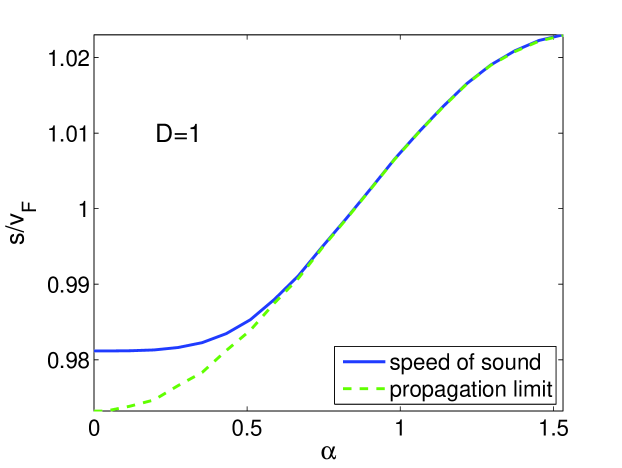
Figure 3: Speed of sound (solid curve) in a dipolar Fermi gas as a function of the angle of propagation $\alpha$ relative to the direction of polarization, for dipolar interaction strength $D=1$. The speed is measured in units of $v_{F}\equiv\hbar k_{F}/m$. The dashed curve represents a lower bound on the speed of any undamped mode. When the two curves merge, zero sound modes are damped and fail to propagate.

As we increase the interaction strength from $D=1$ to $D=3$ (Fig. (4)), there is a noticeable change in the shape of the speed of sound curve. Yet, we still have one propagating mode with some critical angle beyond which zero sound does not propagate.

The deformation of the Fermi surface studied in the previous section contributes somewhat to the change in the speed of sound. It somewhat changes the Fermi surface element and the Fermi velocity $\nu({\bm{k}})$ in Eq (19). However, the main factor giving rise to a change from propagation to damping of zero sound as a function of direction is the anisotropy of the dipolar interaction which directly enters that equation.

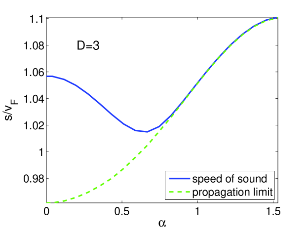
Figure 4: Speed of sound in a dipolar Fermi gas as a function of the angle of propagation $\alpha$, for $D=3$.

For $D>4$ we find that the solution of Eq.( 19) admits complex eigenvalues, in particular an eigenvalue which is purely imaginary and lies on the upper complex plane. This signifies an instability, since according to Eq. (17) such a mode grows exponentially. The imaginary eigenvalue appears first about $D=4.0$ and $\alpha=\pi/2$. Thus, the gas is unstable to growth of density waves in the plan perpendicular to the direction of the dipoles. For $D>4$ we find also additional propagating modes (with real valued frequncies), in particular a transverse mode analog to the transverse mode in superfluid He-3. However, because of the instability, we conclude that these modes could not be experimentally observed, at least unless some additional stabilizing mechanism is introduced.

As noted in the previous section, the compressibility of the gas only becomes infinite at $D=9.5$. However it is physically reasonable that a dipolar gas becomes unstable prior to that. The reason is that the compressibility is a derivative of the pressure, which is an isotropic quantity. But due to the anisotropic interaction, the gas is actually more sensitive.to collapse in a specific direction, i.e, perpendicular to the dipoles. This tends toward the growth of over-density regions where the dipoles are oriented head to tail, lowering the potential energy.

This mechanism is similar to that already long known for homogeneous dipolar Bose gases. A homogeneous Bose gas with a purely dipolar interaction is unstable, but it can be stabilized by the addition of repulsive short range interaction with scattering length $a>0$ ODell04 . In terms of a dimensionless dipolar interaction strength $D_{B}=md^{2}/\hbar^{2}a$, the stability criterion of the homogeneous Bose gas is $D_{B}<3$. Also, from examining the dispersion relation for the Bose gas it can be shown that it becomes first unstable at $D_{B}=3$ due to density waves perpendicular to the direction of polarization. Finally, we note that $D_{B}$ and the dipolar Fermi parameter $D$ (Eq. (14) are related by the simple exchange of the Fermi length scale $1/k_{F}$ with the scattering length $a$. It is interesting to observe that in these respective units, the criteria for the onset of instability in Bose and Fermi gases are very similar in magnitude.

Experimental prospects: We outline some additional considerations regarding the experimental prospects of observing zero sound in dipolar Fermi gas. The condition to have a normal phase is that $T>T_{c}$, where $T_{c}$, the critical temperature for the superfluid transition, is given by $T_{c}\approx 1.44T_{f}\exp\left(-\pi^{3}/(4D)\right)$, with $T_{f}$ the Fermi temperature Baranov02b . At the same time, zero sound attenuation is proportional to $T^{2}/\tau$, where $\tau$ is the relaxation time due to collisions Abrikosov59 . This will set some maximal temperature $T_{m}$ for realistic experimental detection of zero sound. Determining the zero sound attenuation at finite temperature theoretically is a task beyond the scope of this paper , but we note the following: observing zero sound in the normal phase requires $T_{m}>T>T_{c}$, and we thus obtain the condition $D<\pi^{3}/\left(4\log(1.44T_{f}/T_{m})\right)$. As an illustration, if $T_{m}=0.1T_{f}$, we obtain $D<2.9$. Still, even for smaller $T_{m}$, restricting the observation of the zero sound to smaller $D$, it should be possible to see the propagation limited to certain directions only (as in Fig. (3). Finally, the above discussion is based on the requirement that $T>T_{c}$. Nevertheless, we note that, under certain conditions, zero sound of the normal phase can still persist below $T_{c}$, into the superfluid phase Legget66 ; Davis08 .

IV Conclusions

In conclusion, we have studied numerically the deformation of the Fermi surface and zero sound excitations in a homogeneous, single component, degenerate Fermi gas of polar atoms or molecules polarized by an external field. We find that the Fermi surface is described very well by the variational ansatz proposed in Miyakawa08 up to about dipolar interactions strength $D\approx 12.5$, where a compressional instability was predicted. We then study zero sound in the range $D=0-10$. For $D<4$ we find that zero sound can propagate with a longitudinal mode in directions between $\alpha=0$ and some critical $\alpha$ which depends weakly on $D$ but is generally close to $0.6-0.7$ radians ($\alpha$ being the angle between the direction of propagation and the direction of polarization). Beyond this angle, undamped propagation of zero sound is not possible. For $D>4$, we find a complex eigenfrequency indicating that the dipolar gas collapses due to an unstable mode in the direction perpendicular to the dipoles.

Note added: after completion of this work, a work by Chan et al. appeared Chan09 , who also study properties of dipolar Fermi gas, including zero sound.

References

References

- [1] L. D. Landau. Soviet Phys. JETP, 5:101, 1957.
- [2] L.M. Lifshitz and L. P. Pitaevskii. Statistical Physics, Part 2. Butterworth-Heinemann, 1980.
- [3] W. R. Abel, A. C. Anderson, and J. C. Wheatley. Phys. Rev. Lett., 17:74, 1966.
- [4] Pat R. Roach and J. B. Ketterson. Phys. Rev. Lett., 36:736, 1976.
- [5] T. Lahaye, T. Koch, B. Frohlich, M. Fattori, J. Metz, A. Griesmaier, S. Giovanazzi, and T. Pfau. Nature, 448:7154, 2007.
- [6] T. Koch, T. Lahaye, J. Metz, B. Frohlich, A. Griemaier, and T. Pfau. Nauture Physics, 4:218, 2008.
- [7] T. Lahaye, J. Metz, B. Frohlich, T. Koch, M. Meister, A. Griesmaier, T. Pfau, H. Saito, Y. Kawaguchi, and M. Ueda. Phys. Rev. Lett., 101:080401, 2008.
- [8] T. Lahaye, C. Menotti, L. Santos, M. Lewenstein, and T. Pfau. arXiv:0905.0386, 2009.
- [9] S. Ospelkaus, A. Pe’er, K.-K. Ni, J. J. Zirbel, B. Neyenhuis, S. Kotochigova, P. S. Julienne, J. Ye, and D. S. Jin. Nature Physics, 4:622, 2008.
- [10] K.-K. Ni, S. Ospelkaus, M. H. G. de Miranda, A. Pe’er, B. Neyenhuis, J. J. Zirbel, S. Kotochigova, P. S. Julienne, D. S Jin, and J. Ye. Science, 322:231, 2008.
- [11] K. Góral, B.-G. Englert, and K. Rza̧żewski. Phys. Rev. A, 63:033606, 2001.
- [12] T. Miyakawa T. Sogo and H. Pu. Phys. Rev. A., 77:061603, 2008.
- [13] T. Sogo, L. He, T. Miyakawa, S. Yi, H. Lu, and H. Pu. arXiv:0812.0948, 2008.
- [14] Benjamin M. Fregoso, Kai Sun, Eduardo Fradkin, and Benjamin L. Lev. arXiv:0902.0739, 2009.
- [15] M. A. Baranov, M. S. Marénko, Val. S. Rychkov, and G. V. Shlyapnikov. Phys. Rev. A, 66:013606, 2002.
- [16] M. A Baranov, L. Dobrek, and M. Lewenstein. Phys. Rev. Lett., 92:250403, 2004.
- [17] Giovanni Mazzarella, Luca Salasnich, and Flavio Toigo. Phys. Rev. A, 79:023615, 2009.
- [18] S. Giorgini, Lev P. Pitaevskii, and Sandro Stringari. Rev. Mod. Phys., 80:1215, 2008.
- [19] John W. Negale and Henri Orland. Quantum Many-Particle Systems. Addison-Wesely Publishing Compnay, 1988.
- [20] D. H. J. O’Dell, S. Giovanazzi, and C. Eberlein. Phys. Rev. Lett., 92:250401, 2004.
- [21] A. A. Abrikosov and I. M. Khalatnikov. Reports on Progress in Physics, 22:329, 1959.
- [22] A. J. Legget. Physical Review, 147:119, 1966.
- [23] J. P. Davis, J. Pollanen, H. Choi, J. A. Sauls, and A. B. Vorontsov. Phys. Rev. Lett., 101:085301, 2008.
- [24] Ching-Kit Chan, Congjun Wu, Wei cheng Lee, and S. Das Sarma. arXiv:0906.4403, 2009.