The photodissociation and chemistry of CO isotopologues: applications to interstellar clouds and circumstellar disks

Abstract

Aims. Photodissociation by UV light is an important destruction mechanism for carbon monoxide (CO) in many astrophysical environments, ranging from interstellar clouds to protoplanetary disks. The aim of this work is to gain a better understanding of the depth dependence and isotope-selective nature of this process.

Methods. We present a photodissociation model based on recent spectroscopic data from the literature, which allows us to compute depth-dependent and isotope-selective photodissociation rates at higher accuracy than in previous work. The model includes self-shielding, mutual shielding and shielding by atomic and molecular hydrogen, and it is the first such model to include the rare isotopologues C¹⁷O and ¹³C¹⁷O. We couple it to a simple chemical network to analyse CO abundances in diffuse and translucent clouds, photon-dominated regions, and circumstellar disks.

Results. The photodissociation rate in the unattenuated interstellar radiation field is $2.6\times 10^{-10}$ s^-1, 30% higher than currently adopted values. Increasing the excitation temperature or the Doppler width can reduce the photodissociation rates and the isotopic selectivity by as much as a factor of three for temperatures above 100 K. The model reproduces column densities observed towards diffuse clouds and PDRs, and it offers an explanation for both the enhanced and the reduced $N(^{12}\mathrm{CO})/N(^{13}\mathrm{CO})$ ratios seen in diffuse clouds. The photodissociation of C¹⁷O and ¹³C¹⁷O shows almost exactly the same depth dependence as that of C¹⁸O and ¹³C¹⁸O, respectively, so $\@element[17]{\mathrm{O}}$ and $\@element[18]{\mathrm{O}}$ are equally fractionated with respect to $\@element[16]{\mathrm{O}}$. This supports the recent hypothesis that CO photodissociation in the solar nebula is responsible for the anomalous $\@element[17]{\mathrm{O}}$ and $\@element[18]{\mathrm{O}}$ abundances in meteorites. Grain growth in circumstellar disks can enhance the $N(^{12}\mathrm{CO})/N(\mathrm{C}^{17}\mathrm{O})$ and $N(^{12}\mathrm{CO})/N(\mathrm{C}^{18}\mathrm{O})$ ratios by a factor of ten relative to the initial isotopic abundances.

1 Introduction

Carbon monoxide (CO) is one of the most important molecules in astronomy. It is second in abundance only to molecular hydrogen (H₂) and it is the main gas-phase reservoir of interstellar carbon. Because it is readily detectable and chemically stable, CO and its less abundant isotopologues are the main tracers of the gas properties, structure and kinematics in a wide variety of astrophysical environments (for recent examples, see Dame et al. 2001; Najita et al. 2003; Wilson et al. 2005; Greve et al. 2005; Leroy et al. 2005; Huggins et al. 2005; Bayet et al. 2006; Oka et al. 2007; Narayanan et al. 2008). In particular, the pure rotational lines at millimetre wavelengths are often used to determine the total gas mass. This requires knowledge of the CO–H₂ abundance ratio, which may differ by several orders of magnitude from one object to the next (Lacy et al. 1994; Burgh et al. 2007; Panić et al. 2008). If isotopologue lines are used, the isotopic ratio enters as an additional unknown.

CO also controls much of the chemistry in the gas phase and on grain surfaces, and is a precursor to more complex molecules. In photon-dominated regions (PDRs), dark cores and shells around evolved stars, the amount of carbon locked up in CO compared with that in atomic C and C⁺ determines the abundances of small and large carbon-chain molecules (e.g., Millar et al. 1987; Jansen et al. 1995; Aikawa & Herbst 1999; Brown & Millar 2003; Teyssier et al. 2004; Cernicharo 2004; Morata & Herbst 2008). CO ice on the surfaces of grains can be hydrogenated to more complex saturated molecules such as CH₃OH (e.g., Charnley et al. 1995; Watanabe & Kouchi 2002), so the partioning of CO between the gas and grains is important for the overall chemical composition as well (e.g., Caselli et al. 1993; Rodgers & Charnley 2003; Doty et al. 2004; Garrod & Herbst 2006).

A key process in controlling the gas-phase abundance of ¹²CO and its isotopologues is photodissociation by ultraviolet (UV) photons. This is governed entirely by discrete absorptions into predissociative excited states; any possible contributions from continuum channels are negligible (Hudson 1971; Fock et al. 1980; Letzelter et al. 1987; Cooper & Kirby 1987). Spectroscopic measurements in the laboratory at increasingly higher spectral resolution have made it possible for detailed photodissociation models to be constructed (Solomon & Klemperer 1972; Bally & Langer 1982; Glassgold et al. 1985; van Dishoeck & Black 1986; Viala et al. 1988; van Dishoeck & Black 1988, hereafter vDB88; Warin et al. 1996; Lee et al. 1996). The currently adopted photodissociation rate in the unattenuated interstellar radiation field is $2\times 10^{-10}$ s^-1.

Because the photodissociation of CO is a line process, it is subject to self-shielding: the lines become saturated at a ¹²CO column depth of about $10^{15}$ cm^-2, and the photodissociation rate strongly decreases (vDB88; Lee et al. 1996). Bally & Langer (1982) realised this is an isotope-selective effect. Due to their lower abundance, isotopologues other than ¹²CO are not self-shielded until much deeper into a cloud or other object. This results in a zone where the abundances of these isotopologues are reduced with respect to ¹²CO, and the abundances of atomic $\@element[13]{\mathrm{C}}$, $\@element[17]{\mathrm{O}}$ and $\@element[18]{\mathrm{O}}$ are enhanced with respect to $\@element[12]{\mathrm{C}}$ and $\@element[16]{\mathrm{O}}$. For example, the C¹⁷O–¹²CO and C¹⁸O–¹²CO column density ratios towards X Per are a factor of five lower than the elemental oxygen isotope ratios (Sheffer et al. 2002). The ¹³CO–¹²CO ratio along the same line of sight is unchanged from the elemental carbon isotope ratio, indicating that ¹³CO is replenished through low-temperature isotope-exchange reactions. A much larger sample of sources shows $N(^{13}\mathrm{CO})/N(^{12}\mathrm{CO})$ column density ratios both enhanced and reduced by up to a factor of two relative to the elemental isotopic ratio (Sonnentrucker et al. 2007; Burgh et al. 2007; Sheffer et al. 2007). The reduced ratios have so far defied explanation, as all models predict that isotope-exchange reactions prevail over selective photodissociation in translucent clouds.

CO self-shielding has been suggested as an explanation for the anomalous $\@element[17]{\mathrm{O}}$–$\@element[18]{\mathrm{O}}$ abundance ratio found in meteorites (Clayton et al. 1973; Clayton 2002; Lyons & Young 2005; Lee et al. 2008). In cold environments, molecules such as water (H₂O) may be enhanced in heavy isotopes. This so-called isotope fractionation process is due to the difference in vibrational energies of H${}_{2}^{16}$O, H${}_{2}^{17}$O and H${}_{2}^{18}$O, and is therefore mass-dependent. It results in $\@element[18]{\mathrm{O}}$ being about twice as fractionated as $\@element[17]{\mathrm{O}}$. However, $\@element[17]{\mathrm{O}}$ and $\@element[18]{\mathrm{O}}$ are nearly equally fractionated in the most refractory phases in meteorites (calcium-aluminium-rich inclusions, or CAIs), hinting at a mass-independent fractionation mechanism. Isotope-selective photodissociation of CO in the surface of the early circumsolar disk is such a mechanism, because it depends on the relative abundances of the isotopologues and the mutual overlap of absorption lines, rather than on the mass of the isotopologues. The enhanced amounts of $\@element[17]{\mathrm{O}}$ and $\@element[18]{\mathrm{O}}$ are subsequently transported to the planet- and comet-forming zones and eventually incorporated into CAIs. Recent observations of ¹²CO, C¹⁷O and C¹⁸O in two young stellar objects support the hypothesis of CO photodissociation as the cause of the anomalous oxygen isotope ratios in CAIs (Smith et al. 2009). A crucial point in the Lyons & Young model is the assumption that the photodissociation rates of C¹⁷O and C¹⁸O are equal. Our model can test this at least partially.

Detailed descriptions of the CO photodissociation process are also important in other astronomical contexts. The circumstellar envelopes of evolved stars are widely observed through CO emission lines. The measurable sizes of these envelopes are limited primarily by the photodissociation of CO in the radiation field of background starlight (Mamon et al. 1988). Finally, proper treatment of the line-by-line contributions to the photodissociation of CO may affect the analysis of CO photochemistry in the upper atmospheres of planets (Fox & Black 1989).

In this paper, we present an updated version of the photodissociation model from vDB88, based on laboratory experiments performed in the past twenty years (Sect. 2). We expand the model to include C¹⁷O and ¹³C¹⁷O and we cover a broader range of CO excitation temperatures and Doppler widths (Sects. 3 and 4). We rederive the shielding functions from vDB88 and extend these also to higher excitation temperatures and larger Doppler widths (Sect. 5). Finally, we couple the model to a chemical network and discuss the implications for translucent clouds, PDRs and circumstellar disks, with a special focus on the meteoritic $\@element[18]{\mathrm{O}}$ anomaly (Sect. 6).

2 Molecular data

The photodissociation of CO by interstellar radiation occurs through discrete absorptions into predissociated bound states, as first suggested by Hudson (1971) and later confirmed by Fock et al. (1980). Any possible contributions from continuum channels are negligible at wavelengths longer than the Lyman limit of atomic hydrogen (Letzelter et al. 1987; Cooper & Kirby 1987).

Ground-state CO has a dissociation energy of 11.09 eV and the general interstellar radiation field is cut off at 13.6 eV, so knowledge of all absorption lines within that range (911.75–1117.80 Å) is required to compute the photodissociation rate. These data were only partially available in 1988, but ongoing laboratory work has filled in a lot of gaps. Measurements have also been extended to include CO isotopologues, providing more accurate values than can be obtained from theoretical isotopic relations. Table LABEL:tb:moldata-ls lists the values we adopt for ¹²CO.

2.1 Band positions and identifications

Eidelsberg & Rostas (1990, hereafter ER90) and Eidelsberg et al. (1992) redid the experiments of Letzelter et al. (1987) at higher spectral resolution and higher accuracy, and also for ¹³CO, C¹⁸O and ¹³C¹⁸O. They reported 46 predissociative absorption bands between 11.09 and 13.6 eV, many of which were rotationally resolved. Nine of these have a cross section too low to contribute significantly to the overall dissociation rate. The remaining 37 bands are largely the same as the 33 bands of vDB88; bands 1 and 2 of the latter are resolved into four and two individual bands, respectively. Throughout this work, band numbers refer to our numbering scheme (Table LABEL:tb:moldata-ls), unless noted otherwise.

Thanks to the higher resolution and the isotopologue data, ER90 could identify the electronic and vibrational character of the upper states more reliably than Stark et al. in vDB88. The vibrational levels are required to compute the positions for those isotopologue bands that have not been measured directly. Nine of the vDB88 bands (not counting the previously unresolved bands 1 and 2) have a revised $v^{\prime}$ value.

The Eidelsberg et al. (1992) positions ($\nu_{0}$ or $\lambda_{0}$) are the best available for most bands, with an estimated accuracy of 0.1–0.5 cm^-1. Seven of their ¹²CO bands were too weak or diffuse for a reliable analysis, so their positions are accurate only to within 5 cm^-1. Nevertheless, we adopt the Eidelsberg et al. positions for three of these: bands 2A, 6 and 14. The former was blended with band 2B in vDB88, and the other two show a better match with the isotopologue band positions if we take the Eidelsberg et al. values. For the other four weak or diffuse bands, Nos. 4, 15, 19 and 28, we keep the vDB88 positions. Ubachs et al. (1994) further improved the experiments, obtaining an accuracy of about 0.01–0.1 cm^-1, so we adopt their band positions where available. Finally, we adopt the even more accurate positions (0.003 cm^-1 or better) available for the $C1$, $E0$, $E1$ and $L0$ bands (Ubachs et al. 2000; Cacciani et al. 2001, 2002; Cacciani & Ubachs 2004).

Band positions for isotopologues other than ¹²CO are still scarce, although many more are currently known from experiments than in 1988. The $C1$ and $E1$ bands have been measured for all six natural isotopologues, and the $E0$ band for all but ¹³C¹⁷O, at an accuracy of 0.003 cm^-1 (Cacciani et al. 1995; Ubachs et al. 2000; Cacciani et al. 2001; Cacciani & Ubachs 2004). The positions of the $E0$ band are especially important because of its key role in the isotope-selective nature of the CO photodissociation (Sect. 3.3). Positions are known at lower accuracy (0.003–0.5 cm^-1) for an additional 25 C¹⁸O, 30 ¹³CO and 9 ¹³C¹⁸O bands (Eidelsberg et al. 1992; Ubachs et al. 1994; Cacciani et al. 2002); these are included throughout.

We compute the remaining band positions from theoretical isotopic relations. For band $b$ of isotopologue $i$, the position is

$$\nu_{0}(b,i) = \nu_{0}(b,\!{}^{12}\mathrm{CO})+\left[E_{\mathrm{v}}^{\prime}(b,i)-E_{\mathrm{v}}^{\prime\prime}(X,i)\right]-$$ (1)

$$\left[E_{\mathrm{v}}^{\prime}(b,\!{}^{12}\mathrm{CO})-E_{\mathrm{v}}^{\prime\prime}(X,\!{}^{12}\mathrm{CO})\right]\,,$$

with $E_{\mathrm{v}}^{\prime}(b,i)$ and $E_{\mathrm{v}}^{\prime\prime}(X,i)$ the vibrational energy of the excited and ground states, respectively. Hence, we need the vibrational constants ($\omega_{\mathrm{e}}^{\prime}$, $\omega_{\mathrm{e}}x_{\mathrm{e}}^{\prime}$, …) for all the excited states other than the $C\,^{1}\Sigma^{+}$. These have only been determined experimentally for the $E\,^{1}\Pi$ state (Kepa 1988). For the other states, we employ this scheme:

• if it is part of a vibrational series (such as band 30, for which the corresponding $v^{\prime}$=1 band is No. 27), we can derive $\omega_{\mathrm{e}}^{\prime}$ from the difference in $\nu_{0}$;

• else, if it is part of a Rydberg series converging to the $X\,^{2}\Sigma^{+}$ or $A\,^{2}\Pi$ state of CO⁺, we take those constants (Haridass et al. 2000);

• else, we take the constants of ground-state CO (Guelachvili et al. 1983).

The choice for each band and the values of the constants are given in Table LABEL:tb:moldata-ls.

2.2 Rotational constants

The rotational constants ($B_{\mathrm{v}}^{\prime}$ and $D_{\mathrm{v}}^{\prime}$) for each excited state are needed to compute the positions of the individual absorption lines. ER90 provided $B_{\mathrm{v}}^{\prime}$ values for most bands, at an estimated accuracy of better than 1%. Their $D_{\mathrm{v}}^{\prime}$ values are less well constrained and may be off by more than a factor of two. However, this is of little importance for the low-$J$ lines typically involved in the photodissociation of CO. More accurate values ($B_{\mathrm{v}}^{\prime}$ to better than 0.1%, $D_{\mathrm{v}}^{\prime}$ to 10% or better) are available for 12 states from higher-resolution experiments (Eikema et al. 1994; Ubachs et al. 1994, 2000; Cacciani et al. 2001, 2002; Cacciani & Ubachs 2004). Again, the data for isotopologues other than ¹²CO are generally scarce, so we have to compute their constants from theoretical isotopic relations. This increases the uncertainty in $B_{\mathrm{v}}^{\prime}$ to a few per cent. In case of bands 12, 15, 19 and 28, ER90 reported constants for C¹⁸O but not for ¹²CO, so we employ the theoretical relations for the latter. We adopt the vDB88 constants for bands 4 and 14, because they are more accurate than those of ER90. No constants are available for Rydberg bands 2A and 6, so we adopt the constants of the associated CO⁺ states ($A\,^{2}\Pi$ and $X\,^{2}\Sigma^{+}$, respectively).

In seven cases, the rotational constants of the P and R branch ($e$ parity) were found to differ from those of the Q branch ($f$ parity; Ubachs et al. 1994, 2000; Cacciani et al. 2002; Cacciani & Ubachs 2004). For these bands, the $f$ parity values are given in Table LABEL:tb:moldata-ls. Table 2 lists the difference between the $f$ and $e$ values, defined as $q_{\mathrm{v}}^{\prime}=B_{\mathrm{v},e}^{\prime}-B_{\mathrm{v},f}^{\prime}$ and $p_{\mathrm{v}}^{\prime}=D_{\mathrm{v},e}^{\prime}-D_{\mathrm{v},f}^{\prime}$. The uncertainties in $q_{\mathrm{v}}^{\prime}$ and $p_{\mathrm{v}}^{\prime}$ are on the order of 1 and 10%, respectively.

Table 2: Parity-dependent rotational constants for ¹²CO.

Band	$q_{\mathrm{v}}^{\prime}$		$p_{\mathrm{v}}^{\prime}{}^{\mathrm{a}}$		Refs.b
#	(cm-1)		(cm-1)
16	$-2$.	7(-3)	—		1
22	2.	212(-2)	7.	9(-6)	2
23	3.	0(-2)	—		1
25	$-7$.	0(-4)	—		1
26	$-1$.	11(-2)	—		1
31	1.	14(-2)	3.	0(-8)	3
33	1.	196(-2)	2.	1(-7)	4

• Dashes indicate that no measurement is available, so we adopt a value of zero.

• (1) Ubachs et al. (1994); (2) Cacciani et al. (2002); (3) Ubachs et al. (2000); (4) Cacciani & Ubachs (2004)

2.3 Oscillator strengths

ER90 measured the integrated absorption cross sections ($\sigma_{\mathrm{int}}$) for all their bands to a typical accuracy of 20%, but they cautioned that some values, especially for mutually overlapping bands, may be off by up to a factor of two. The oscillator strengths ($f_{\mathrm{v}^{\prime}0}$) derived from these data are different from vDB88 for most bands, sometimes by even more than a factor of two. In addition, there are differences of up to an order of magnitude between the cross sections of ¹²CO and those of the other isotopologues for many bands shortwards of 990 Å. The isotopic differences are likely due in part to the difficulty in determining individual cross sections for strongly overlapping bands, but isotope-selective oscillator strengths in general are not unexpected. For example, they were also observed recently in high-resolution measurements of N₂ (G. Stark, priv. comm.). For CO, the oscillator strengths depend on the details of the interactions between the $J^{\prime}$, $v^{\prime}$ levels of the excited states and other rovibronic levels. These interactions, in turn, depend on the energy levels, which are different between the isotopologues. We adopt the isotope-selective oscillator strengths where available. In case of transitions where no isotopic data exist, we choose to take the value of the isotopologue nearest in mass. This gives the closest match in energy levels and should, in general, also give the closest match in oscillator strengths, which to first order are determined by the Franck-Condon factors.

For ten of our bands, we adopt oscillator strenghts from studies that aimed specifically at measuring this parameter (Federman et al. 2001; Eidelsberg et al. 2004, 2006). Their esimated accuracy is 5–15%. The oscillator strength for the $E0$ band from Federman et al. (2001) is almost twice as large as that of vDB88 and ER90, which appears to be due to an inadequate treatment of saturation effects in the older work. The 2001 value corresponds well to other values derived since 1990. Federman et al. also measured the oscillator strength of the weaker $C1$ band and found it to be the same, within the error margins, as that of vDB88 and ER90. Recent measurements of the $K0$, $L0$ and $E1$ transitions and the four $W$ transitions show larger oscillator strengths than those of vDB88 and ER90 (Eidelsberg et al. 2004, 2006). The new values correspond closely to those of Sheffer et al. (2003), who derived oscillator strengths for eight bands by fitting a synthetic spectrum to Far Ultraviolet Spectroscopic Explorer (FUSE) data taken towards the star HD 203374A. Lastly, the Eidelsberg et al. (2004) value for the $L^{\prime}1$ band is 33% lower than that of vDB88, but very similar to those of ER90 and Sheffer et al. (2003), so we adopt it as well.

We compute the oscillator strengths of individual lines as the product of the appropriate Hönl-London factor and the oscillator strength of the corresponding band (Morton & Noreau 1994). Significant departures from Hönl-London patterns have been reported for many N₂ lines, sometimes even for the lowest rotational levels (Stark et al. 2005, 2008). The oscillator strength measured in one particular N₂ band for the P(22) line was twenty times stronger than that for the P(2) line, due to strong mixing of the upper state with a nearby Rydberg state. For other bands where deviations from Hönl-London factors were observed, the effect was generally less than 50% at $J^{\prime}$=10. Similar deviations are likely to occur for CO, but a lack of experimental data prevents us from including this in our model. Note, however, that large deviations are only expected for specific levels that happen to be strongly interacting with another state. Many hundreds of levels contribute to the photodissociation rate, so the effect of some erroneous individual line oscillator strengths is small.

2.4 Lifetimes and predissociation probabilities

Upon excitation, there is competition between dissociative and radiative decay. A band’s predissociation probability ($\eta$) can be computed if the upper state’s total and radiative lifetimes are known: $\eta=1-\tau_{\mathrm{tot}}/\tau_{\mathrm{rad}}$. ER90 reported total lifetimes (1/$A_{\mathrm{tot}}$) for all their bands, but many of these are no more than order-of-magnitude estimates. Higher-resolution experiments have since produced more accurate values for 17 of our bands (Ubachs et al. 1994, 2000; Cacciani et al. 1998, 2001, 2002; Eidelsberg et al. 2006). In several cases, values that differ by up to a factor of three are reported for different isotopologues. Where available, we take isotope-specific values. Otherwise, we follow the same procedure as for the oscillator strengths, and take the value of the isotopologue nearest in mass.

The total lifetimes of some upper states have been shown to depend on the rotational level (Drabbels et al. 1993; Ubachs et al. 2000; Eidelsberg et al. 2006). In case of ${}^{1}\Pi$ states, a dependence on parity was sometimes observed as well. We include these effects for the five bands in which they have been measured (Table 3).

Table 3: Parity- and rotation-dependent inverse lifetimes for ¹²CO.

Band	$A_{\mathrm{tot},f}{}^{\mathrm{a}}$		$A_{\mathrm{tot},e}{}^{\mathrm{a}}$		Refs.b
#	(s-1)		(s-1)
08	3.	6(11)+4.0(9)$x$	1.	6(11)+1.3(10)$x$	1
c13c	3.	4(10)+7.3(10)$x$	—		2
16	1.	0(11)+1.8(9)$x$	1.	0(11)+3.4(9)$x$	1
22	1.	83(9)	1.	91(9)+1.20(9)$x$	3
25	1.	2(10)	1.	2(10)+2.4(9)$x$	1

• $x$ stands for $J^{\prime}(J^{\prime}+1)$.

• (1) Eidelsberg et al. (2006); (2) Ubachs et al. (1994); (3) Drabbels et al. (1993).

• This is a ${}^{1}\Sigma^{+}$ upper state, so there is no distinction between $e$ and $f$ parity.

Recent experiments by Chakraborty et al. (2008) suggest isotope-dependent photodissociation rates for the $E0$, $E1$, $K0$ and $W2$ bands. These have been interpreted to imply different predissociation probabilities of individual lines of the various isotopologues due to a near-resonance accidental predissociation process. Similar effects have been reported for ClO₂ and CO₂ (Lim et al. 1999; Bhattacharya et al. 2000). In this process, the bound-state levels into which the UV absorption takes place do not couple directly with the continuum of a dissociative state. Instead, they first transfer population to another bound state, whose levels happen to lie close in energy. For the CO $E1$ state, this process was rotationally resolved by Ubachs et al. (2000) for all naturally occurring isotopologues and shown to be due to spin-orbit interaction with the $k\,^{3}\Pi$ $v^{\prime}$=6 state, which in turn couples with a repulsive state. The predissociation rates of the $E1$ state are found to increase significantly due to this process, but only for specific $J^{\prime}$ levels that accidentally overlap. For example, interaction occurs at $J^{\prime}$=7, 9 and 12 for ¹²CO, but at $J^{\prime}$=1 and 6 for ¹³C¹⁸O. Since the dissociation probabilities for the $E1$ state due to direct predissociation were already high, $\eta=0.96$, this increase in dissociation rate only has a very minor effect (Cacciani et al. 1998). Moreover, under astrophysical conditions a range of $J^{\prime}$ values are populated, so that the effect of individual levels is diluted. Since Chakraborty et al. did not derive line-by-line molecular parameters, we cannot easily incorporate their results into our model. In Sect. 6.3, we show that our results do not change significantly when we include the proposed effects in an ad-hoc way.

The radiative lifetime of an excited state is a sum over the decay into all lower-lying levels, including the $A\,^{1}\Pi$ and $B\,^{1}\Sigma^{+}$ electronic states and the $v^{\prime}$$\neq$0 levels of the ground state. The total decay rate to the ground state is obtained by summing the oscillator strengths from Table LABEL:tb:moldata-ls for each vibrational series (Morton & Noreau 1994; Cacciani et al. 1998). Theoretical work by Kirby & Cooper (1989) showed that transitions to electronic states other than the ground state contribute about 1% of the overall radiative decay rate for the $C$ state and about 8% for the $E$ state. No data are available for the excited states at higher energies. Fortunately, the radiative decay rate from these higher states to the ground state is small compared to the dissociation rate, so an uncertainty of $\sim$10% will not affect the $\eta$ values.

The predissociation probabilities thus computed are nearly identical to those of vDB88: the largest difference is a 10% decrease for the $C1$ band. This is due to the larger oscillator strength now adopted.

There have been suggestions that the $C0$ state can also contribute to the photodissociation rate. Cacciani et al. (2001) measured upper-state lifetimes in the $C0$ and $C1$ states for several CO isotopologues. For the $v^{\prime}$=0 state of ¹³CO they found a total lifetime of 1770 ps, consistent with a value of 1780 ps for ¹²CO, but different from the lifetime of 1500 ps in ¹³C¹⁸O. Although the three values agree within the mutual uncertainties of 10–15% on each measurement, Cacciani et al. suggested that the heaviest species, ¹³C¹⁸O, has a predissociation yield of $\eta=0.17$ rather than zero if the measurements are taken at face value and if the radiative lifetime of the $C0$ state is presumed to be 1780 ps for all three species. The accurate absorption oscillator strength measured by Federman et al. (2001) for the $C0$ band, $0.123\pm 0.016$, implies a radiative lifetime that can be no longer than 1658 ps at the lower bound of measurement uncertainty in $f_{\mathrm{v}^{\prime}0}$. Taken together, the lifetime measurements of Cacciani et al. and the absorption measurements of Federman et al. favour a conservative conclusion that the dissociation yield is zero for each of these three isotopologues. We assume the $C0$ band is also non-dissociative in C¹⁷O, C¹⁸O and ¹³C¹⁷O; this is consistent with earlier studies (e.g., vDB88; ER90; Morton & Noreau 1994).

2.5 Atomic and molecular hydrogen

Lines of atomic and molecular hydrogen (H and H₂) form an important contribution to the overall shielding of CO. As in vDB88, we include H Lyman lines up to $n$=50 and H₂ Lyman and Werner lines (transitions to the $B\,^{1}\Sigma_{u}^{+}$ and $C\,^{1}\Pi_{u}$ states) from the $v^{\prime\prime}$=0, $J^{\prime\prime}$=0–7 levels of the electronic ground state. We adopt the line positions, oscillator strengths and lifetimes from Abgrall et al. (1993a, b), as compiled for the freely available Meudon PDR code (Le Bourlot et al. 1993; Le Petit et al. 2002, 2006). Ground-state rotational constants, required to compute the level populations, come from Jennings et al. (1984).

3 Depth-dependent photodissociation

3.1 Default model parameters

The simplest way of modelling the depth-dependent photodissociation involves dividing a one-dimensional model of an astrophysical object, irradiated only from one side, into small steps, in which the photodissociation rates can be assumed constant. We compute the abundances from the edge inwards, so that at each step we know the columns of CO, H, H₂ and dust shielding the unattenuated radiation field.

Following vDB88, Le Bourlot et al. (1993), Lee et al. (1996) and Le Petit et al. (2006), we treat the line and continuum attenuation separately. For each of our 37 CO bands, we include all lines originating from the first ten rotational levels ($J^{\prime\prime}$=0–9) of the $v^{\prime\prime}$=0 level of the electronic ground state. That results in 855 lines per isotopologue. In addition, we have 48 H lines and 444 H₂ lines, for a total of 5622. We use an adaptive wavelength grid that resolves all lines without wasting computational time on empty regions. For typical model parameters, the wavelength range from 911.75 to 1117.80 Å is divided into $\sim$47,000 steps.

We characterise the population distribution of CO over the rotational levels by a single temperature, $T_{\mathrm{ex}}(\mathrm{CO})$. The H₂ population requires a more detailed treatment, because UV pumping plays a large role for the $J^{\prime\prime}$¿4 levels (van Dishoeck & Black 1986). We populate the $J^{\prime\prime}$=0–3 levels according to a single temperature, $T_{\mathrm{ex}}(\mathrm{H}_{2})$, and adopt fixed columns of $4\times 10^{15}$, $1\times 10^{15}$, $2\times 10^{14}$ and $1\times 10^{14}$ cm^-2 for $J^{\prime\prime}$=4–7. This reproduces observed translucent cloud column densities to within a factor of two (van Dishoeck & Black 1986 and references therein). The $J^{\prime\prime}$¿4 population scales with the UV intensity, so we re-evaluate this point for PDRs and circumstellar disks in Sects. 6.2 and 6.3.

The line profiles of CO, H₂ and H are taken to be Voigt functions, with default Doppler widths ($b$) of 0.3, 3.0 and 5.0 km s^-1, respectively. We adopt Draine (1978) as our standard unattenuated interstellar radiation field.

3.2 Unshielded photodissociation rates

We obtain an unshielded CO photodissociation rate of $2.6\times 10^{-10}$ s^-1. This rate is 30% higher than that of vDB88, due to the generally larger oscillator strengths in our data set. The new data for bands 33 and 24 (the $E0$ and $K0$ transitions) have the largest effect: they account for 63 and 21% of the overall increase. Clearly, the rate depends on the choice of radiation field. If we adopt Habing (1968), Gondhalekar et al. (1980) or Mathis et al. (1983) instead of Draine (1978), the photodissociation rate becomes 2.0, 2.0 or $2.3\times 10^{-10}$ s^-1, respectively. vDB88 reported the same relative differences between these three fields.

Table 4: Relative and absolute shielding effects for the ten most important bands in the $ζ$ Oph cloud.^a

Band	33	28	24	23	22	20	19	16	15	13	Totalc
$\lambda_{0}$ (Å)b	1076.1	985.6	970.4	968.9	968.3	956.2	950.0	941.2	940.0	933.1
12CO
Edge (%)d	32.2000	04.7000	08.7000	03.0000	03.6000	03.4000	04.3000	05.1000	03.5000	03.1000	7.8(-10)
Centre (%)d	02.8000	00.4000	05.7000	09.3000	00.8000	12.1000	13.8000	06.1000	11.0000	07.0000	7.5(-11)
Shieldinge	00.0084	00.0072	00.0630	00.3000	00.0220	00.3400	00.3100	00.1200	00.3000	00.2200	0.10(-0)
C17O
Edge (%)	32.0000	04.7000	08.7000	03.0000	03.6000	03.4000	04.3000	05.1000	03.5000	03.1000	7.8(-10)
Centre (%)	22.0000	00.1000	05.3000	03.5000	00.8000	08.7000	10.3000	14.2000	09.1000	02.4000	2.4(-10)
Shielding	00.2100	00.0067	00.1900	00.3600	00.0650	00.7900	00.7400	00.8500	00.8100	00.2300	0.31(-0)
C18O
Edge (%)	31.5000	05.1000	06.2000	01.5000	04.9000	03.7000	04.7000	05.2000	03.8000	03.4000	7.2(-10)
Centre (%)	35.3000	00.1000	04.7000	02.6000	07.8000	03.3000	07.7000	08.1000	05.9000	03.0000	3.7(-10)
Shielding	00.5800	00.0067	00.3900	00.8800	00.8200	00.4600	00.8300	00.8000	00.8100	00.4500	0.52(-0)
13CO
Edge (%)	28.1000	06.5000	08.3000	01.8000	05.2000	03.4000	04.3000	04.9000	03.9000	02.4000	7.8(-10)
Centre (%)	18.5000	00.0000	05.3000	04.4000	11.2000	04.1000	10.7000	04.4000	09.1000	00.8000	2.8(-10)
Shielding	00.2300	00.0007	00.2300	00.8700	00.7600	00.4200	00.8700	00.3200	00.8300	00.1300	0.35(-0)
13C17O
Edge (%)	28.0000	06.3000	08.3000	01.8000	05.2000	03.4000	04.3000	04.9000	03.9000	02.4000	7.8(-10)
Centre (%)	32.5000	00.0000	07.4000	02.9000	07.5000	05.0000	07.2000	08.5000	06.1000	01.0000	4.2(-10)
Shielding	00.6300	00.0007	00.4800	00.8800	00.7900	00.7800	00.9100	00.9400	00.8500	00.2400	0.54(-0)
13C18O
Edge (%)	30.1000	07.0000	05.9000	01.5000	04.7000	03.6000	04.4000	05.0000	04.0000	02.4000	7.5(-10)
Centre (%)	39.0000	00.0000	05.8000	02.4000	05.7000	01.7000	07.5000	08.5000	06.3000	01.7000	4.1(-10)
Shielding	00.7100	00.0007	00.5400	00.8700	00.6700	00.2600	00.9200	00.9400	00.8500	00.3800	0.55(-0)

• See the text for the adopted column densities, Doppler widths, excitation temperatures and radiation field.

• ¹²CO band head position.

• Total photodissociation rate in s^-1 at the edge and the centre, and the shielding factor at the centre.

• Relative contribution per band to the overall photodissociation rate at the edge and the centre of the cloud.

• Shielding factor per band: the absolute contribution at the centre divided by the absolute contribution at the edge.

3.3 Shielding by CO, H₂ and H

Self-shielding, shielding by H, H₂ and the other CO isotopologues, and continuum shielding by dust all reduce the photodissociation rates inside a cloud or other environment relative to the unshielded rates. For a given combination of column depths ($N$) and visual extinction ($A_{\mathrm{V}}$), the photodissociation rate for isotopologue $i$ is

$$k_{i}=\chi k_{0,i}\Theta_{i}\exp(-\gamma A_{\mathrm{V}})\,,$$ (2)

with $\chi$ a scaling factor for the UV intensity and $k_{0,i}$ the unattenuated rate in a given radiation field. The shielding function $\Theta_{i}$ accounts for self-shielding and shielding by H, H₂ and the other CO isotopologues; tabulated values for some typical model parameters are presented in Tables 5–8. The dust extinction term, $\exp(-\gamma A_{\mathrm{V}})$, is discussed in Sect. 3.4. Equation (2) assumes the radiation is coming from all directions. If this is not the case, such as for a cloud irradiated only from one side, $k_{0,i}$ should be reduced accordingly.

For now, we ignore shielding by dust and compute the depth-dependent photodissociation rates due to line shielding only. Our test case is the centre of the diffuse cloud towards the star $\zeta$ Oph. The observed column densities of H, H₂, ¹²CO and ¹³CO are $5.2\times 10^{20}$, $4.2\times 10^{20}$, $2.5\times 10^{15}$ and $1.5\times 10^{13}$ cm^-2 (van Dishoeck & Black 1986; Lambert et al. 1994), and we assume C¹⁷O, C¹⁸O, ¹³C¹⁷O and ¹³C¹⁸O column densities of $4.1\times 10^{11}$, $1.6\times 10^{12}$, $5.9\times 10^{9}$ and $2.3\times 10^{10}$ cm^-2, consistent with observational constraints. For the centre of the cloud, we adopt half of these values. We set $b(\mathrm{CO})=0.48$ km s^-1 and $T_{\mathrm{ex}}(\mathrm{CO})=4.2$ K (Sheffer et al. 1992), and we populate the H₂ rotational levels explicitly according to the observed distribution. The cloud is illuminated by three times the Draine field ($\chi=3$).

Table 4 lists the relative contribution of the most important bands at the edge and centre for each isotopologue, as well as the overall photodissociation rate at each point. The column densities are small, but isotope-selective shielding already occurs: the ¹²CO rate at the centre is lower than that of the other isotopologues by factors of three to six.

The $E0$ band is the most important contributor at the edge. This was also found by vDB88, but the higher oscillator strength now adopted makes it even stronger. Going to the centre, it saturates rapidly for ¹²CO: its absolute contribition to the total dissociation rate decreases by two orders of magnitude, and it goes from the strongest band to the 12th strongest band. The five strongest bands at the centre are the same as in vDB88: Nos. 13, 15, 19, 20 and 23.

Figure 1 illustrates the isotope-selective shielding. The left panel is centred on the R(1) line of the $E0$ band (No. 33 from Table LABEL:tb:moldata-ls). This line is fully saturated in ¹²CO and the relative intensity of the radiation field ($I/I_{0}$, with $I_{0}$ the intensity at the edge of the cloud) goes to zero. ¹³CO and C¹⁸O also visibly reduce the intensity, to $I/I_{0}=0.50$ and 0.72, but the other three isotopologues are not abundant enough to do so. Consequently, these three are not self-shielded in the $\zeta$ Oph cloud, but they are shielded by ¹²CO, ¹³CO and C¹⁸O. The weaker shielding of ¹³C¹⁷O and ¹³C¹⁸O in the $E0$ band compared to C¹⁷O is due to their lines having less overlap with the ¹²CO lines.

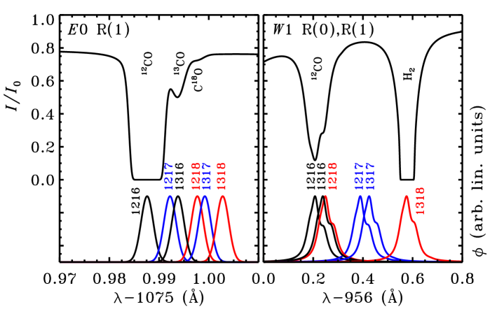
Figure 1: Relative intensity of the radiation field ($I/I_{0}$) and intrinsic line profiles for the six CO isotopologues ($\phi$, in arbitrary linear units) at the centre of the $\zeta$ Oph cloud in two wavelength ranges.

The right panel of Fig. 1 contains the R(0) line of the $W1$ band (No. 20), with the R(1) line present as a shoulder on the red wing. Also visible is the saturated $B13$ R(2) line of H₂ at 956.58 Å. The $W1$ band is weaker than the $E0$ band, so ¹²CO is the only isotopologue to cause any appreciable reduction in the radiation field and to be (partially) self-shielded. The shielding of the other five isotopologues is dominated by overlap with the ¹²CO and H₂ lines. This figure also shows the need for accurate line positions: if the ¹³C¹⁸O line were shifted by 0.1 Å in either direction, it would no longer overlap with the H₂ line and be less strongly shielded. Note that the position of the $W1$ band has only been measured for ¹²CO, ¹³CO and C¹⁸O, so we have to compute the position for the other isotopologues from theoretical isotopic relations. This causes the C¹⁷O line to appear longwards of the C¹⁸O line.

3.4 Continuum shielding by dust

Dust can provide a very strong attenuation of the radiation field. This effect is largely independent of wavelength for the 912–1118 Å radiation available to dissociate CO, so it affects all isotopologues to the same extent. It can be expressed as an exponential function of the visual extinction, as expressed in Eq. (2). For typical interstellar dust grains (radius of 0.1 $\mu$m and optical properties from Roberge et al. 1991), the extinction coefficient $\gamma$ is 3.53 for CO (van Dishoeck et al. 2006). Larger grains have less opacity in the UV and do not shield CO as strongly. For ice-coated grains with a mean radius of 1 $\mu$m, appropriate for circumstellar disks (Jonkheid et al. 2006), the extinction coefficient is only 0.6. The effects of dust shielding are discussed more fully in Sect. 6.

Photodissociation of CO may still take place even in highly extincted regions. Cosmic rays or energetic electrons generated by cosmic rays can excite H₂, allowing it to emit in a multitude of bands, including the Lyman and Werner systems (Prasad & Tarafdar 1983). The resulting UV photons can dissociate CO at a rate of about $10^{-15}$ s^-1 (Gredel et al. 1987), independent of depth. That is enough to increase the atomic C abundance by some three orders of magnitude compared to a situation where the photodissociation rate is absolutely zero. The cosmic-ray-induced photodissociation rate is sensitive to the spectroscopic constants of CO, especially where it concerns the overlap between CO and H₂ lines, so it would be interesting to redo the calculations of Gredel et al. with the new data from Table LABEL:tb:moldata-ls. However, that is beyond the scope of this paper.

3.5 Uncertainties

The uncertainties in the molecular data are echoed in the model results. When coupled to a chemical network, as in Sect. 6, the main observables produced by the model are the column densities of the CO isotopologues for a given astrophysical environment. The accuracy of the photodissociation rates is only relevant in a specific range of depths; in the average interstellar UV field, this range runs from an $A_{\mathrm{V}}$ of $\sim$0.2 to $\sim$2 mag. Photoprocesses are so dominant at lower extinctions and so slow at higher extinctions that the exact rate does not matter. In the intermediate regime, both the absolute photodissociation rates and the differences between the rates for individual isotopologues are important. The oscillator strengths are the key variable in both cases and these are generally known rather accurately. Taking account of the experimental uncertainties in the band oscillator strengths and of the theoretical uncertainties in computing the properties for individual lines, and identifying which bands are important contributors (Table 4), we estimate the absolute photodissociation rates to be accurate to about 20%. This error margin carries over into the absolute CO abundances and column densities for the $A_{\mathrm{V}}\approx 0.2$–2 mag range when the rates are put into a chemical model. The accuracy on the rates and abundances of the isotopologues relative to each other is estimated to be about 10% when summed over all states, even when we allow for the kind of isotope-specific predissociation probabilities suggested by Chakraborty et al. (2008).

4 Excitation temperature and Doppler width

The calculations of vDB88 were only done for low excitation temperatures of CO and H₂. Here, we extend this work to higher temperatures, as required for PDRs and disks, and we re-examine the effect of the Doppler widths of CO, H₂ and H on the photodissociation rates. We first treat four cases separately, increasing either $T_{\mathrm{ex}}(\mathrm{CO})$, $b(\mathrm{CO})$, $T_{\mathrm{ex}}(\mathrm{H}_{2})$ or $b(\mathrm{H}_{2})$. At the end of this section we combine these effects in a grid of excitation temperatures and Doppler widths. As a template model we take the centre of the $\zeta$ Oph cloud, with column densities and other parameters as described in Sect. 3.3.

4.1 Increasing $T_{\mathrm{ex}}(\mathrm{CO})$

As the excitation temperature of CO increases, additional rotational levels are populated and photodissociation is spread across more lines. Figure 2 visualises this for band 13 of ¹²CO. At 4 K, only four lines are active: the R(0), R(1), P(1) and P(2) lines at 933.02, 932.98, 933.09 and 933.12 Å. The R(0) and P(1) lines are both fully self-shielded at the line centre. Going to 16 K, the R(0) line loses about 70% of its intrinsic intensity and ceases to be self-shielding. In addition, the R(2), P(3) and higher-$J$ lines start to absorb. The combination of less saturated low-$J$ lines and more active higher-$J$ lines yields a 39% higher photodissociation rate at 16 K compared to 4 K.

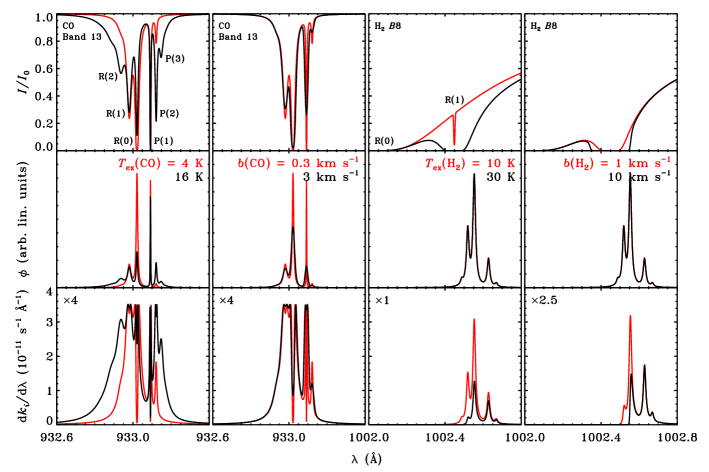
Figure 2: Illustration of the effect of increasing $T_{\mathrm{ex}}(\mathrm{CO})$, $b(\mathrm{CO})$, $T_{\mathrm{ex}}(\mathrm{H}_{2})$ or $b(\mathrm{H}_{2})$ (from left to right) in our $\zeta$ Oph cloud model (Sect. 3.3). Top: relative intensity of the radiation field, including absorption by only ¹²CO (left two panels) or H₂ (right two panels). Middle: intrinsic line profile for band 13 (933.1 Å) or 30 (1002.6 Å) of ¹²CO. Bottom: photodissociation rate per unit wavelength, multiplied by a constant as indicated.

A higher CO excitation temperature has the same favourable effect for ¹³CO, which is partially self-shielded at the centre of the $\zeta$ Oph cloud. Its photodissociation rates increase by 16% when going from 4 to 16 K. C¹⁸O is also partially self-shielded, but less so than ¹³CO, so the favourable effect is smaller. At the same time, it suffers from increased overlap by ¹²CO. The net result is a small increase in the photodissociation rate of 0.2%.

The two heaviest isotopologues, ¹³C¹⁷O and ¹³C¹⁸O, are not abundant enough to be self-shielded. Their $J^{\prime\prime}$¡2 lines generally have little overlap with the corresponding ¹²CO lines, especially in the $E0$ band near 1076 Å. This band, whose lines are amongst the narrowest in our data set, is the strongest contributor to the photodissociation rate at the centre of the cloud for ¹³C¹⁷O and ¹³C¹⁸O (Table 4). In fact, its narrow lines are part of the reason it is the strongest contributor. The $J^{\prime\prime}$=3 and 4 lines that become active at 16 K do have some overlap with ¹²CO. Without the favourable effect of less self-shielding, this causes the photodissociation rate for ¹³C¹⁷O and ¹³C¹⁸O to decrease for higher excitation temperatures. The change is only small, though: 0.4% for ¹³C¹⁷O and 2% for ¹³C¹⁸O.

Finally, C¹⁷O experiences an increase of 18% in its photodissociation rate. Its lines lie closer to those of ¹²CO than do the ¹³C¹⁷O and ¹³C¹⁸O lines, so it is generally more strongly shielded. At 4 K, most of the shielding is due to the saturated R(0) lines of ¹²CO. These become partially unsaturated at higher $T_{\mathrm{ex}}(\mathrm{CO})$, so the corresponding R(0) lines of C¹⁷O become a stronger contributor to the photodissociation rate, even though the shift towards higher-$J$ lines make them intrinsically weaker. Overall, increasing $T_{\mathrm{ex}}(\mathrm{CO})$ from 4 to 16 K thus results in a higher C¹⁷O photodissociation rate.

4.2 Increasing $b(\mathrm{CO})$

The width of the absorption lines is due to Doppler broadening and natural (or lifetime) broadening. The integrated intensity in each line remains the same when $b(\mathrm{CO})$ increases, so a larger width is accompanied by a lower peak intensity. The resulting reduction in self-shielding then causes a higher ¹²CO photodissociation rate, as shown in Fig. 2 for band 13. However, the effect is rather small because the Doppler width is smaller than the natural width for most lines at typical $b$ values. Natural broadening is the dominant broadening mechanism up to $b(\mathrm{CO})\approx 6\times 10^{-12}A_{\mathrm{tot}}$, with both parameters in their normal units. The R(0) line of band 13 has an inverse lifetime of $1.8\times 10^{11}$ s^-1 (Tables LABEL:tb:moldata-ls and 3), so Doppler broadening becomes important at about 1 km s^-1. From 0.3 to 3 km s^-1, as in Fig. 2, the line width only increases by a factor of 1.9. Integrated over all lines, the ¹²CO photodissociation rate becomes 26% higher.

The rates of the other five isotopologues decrease along this $b(\mathrm{CO})$ interval due to increased shielding by the $E0$ lines of ¹²CO. With an inverse lifetime of only $1\times 10^{9}$ s^-1, Doppler broadening is this band’s dominant broadening mechanism in the regime of interest. A tenfold increase in the Doppler parameter from 0.3 to 3 km s^-1 results in a nearly tenfold increase in the line widths. At 0.3 km s^-1, the $E0$ lines of ¹²CO are still sufficiently narrow that they do not strongly shield the lines of the other isotopologues. This is no longer the case at 3 km s^-1. ¹³CO still benefits somewhat from reduced self-shielding in other bands, but it is not enough to overcome the reduced strength of the $E0$ band, and its photodissociation rates decrease by 2%. The decrease is 13% for C¹⁷O and 26–28% for the remaining three isotopologues. The relatively small decrease for C¹⁷O is due to its $E0$ band being already partially shielded by ¹²CO at 0.3 km s^-1, so the stronger shielding at 3 km s^-1 has less of an effect.

4.3 Increasing $T_{\mathrm{ex}}(\mathrm{H}_{2})$ or $b(\mathrm{H}_{2})$

Increasing the excitation temperature of H₂, while keeping the CO parameters constant, results in a decreased photodissociation rate for all six isotopologues. The cause, as again illustrated in Fig. 2, is the activation of more H₂ lines. At $T_{\mathrm{ex}}(\mathrm{H}_{2})=10$ K, the R(1) line of the $B8$ band at 1002.45 Å is very narrow and does not shield the $F0$ band (No. 30) of the CO isotopologues. (The continuum-like shielding visible in Fig. 2 is due to the strongly saturated $B8$ R(0) line at 1001.82 Å.) It becomes much more intense at 30 K and widens due to being saturated, thereby shielding part of the $F0$ band. The same thing happens to other CO bands, resulting in an overall rate decrease of 0.6–2.5%. There is no particular trend visible amongst the isotopologues; the magnitude of the rate change depends purely on the chance that a given CO band overlaps with an H₂ line.

Similar decreases of one or two percent in the CO photodissociation rates are seen when the H₂ Doppler width is changed from 1 to 10 km s^-1. As the H₂ lines become broader, the amount of overlap with CO increases across the entire wavelength range. As an example, Fig. 2 shows again the 1002.0–1002.8 Å region, where the $B8$ R(1) line of H₂ further reduces the contribution of the $F0$ band to the ¹²CO photodissociation rate.

4.4 Grid of $T_{\mathrm{ex}}$ and $b$

We now combine the four individual cases into a grid of excitation temperatures and Doppler widths to see how they influence each other. $T_{\mathrm{ex}}(\mathrm{CO})$ is raised from 4 to 512 K in steps of factors of two. The $v^{\prime\prime}$=1 vibrational level of ¹²CO lies at 2143 cm^-1 above the $v^{\prime\prime}$=0 level, so it starts to be thermally populated at $\sim$500 K. No data are available on dissociative transitions out of this level, so we choose not to go to higher excitation temperatures. We increase the range of rotational levels up to $J^{\prime\prime}$=39, at 2984 cm^-1 above the $J^{\prime\prime}$=0 level for ¹²CO. At $T_{\mathrm{ex}}(\mathrm{CO})=512$ K, the normalised population distribution peaks at $J^{\prime\prime}$=9 and decreases to $9.7\times 10^{-5}$ at $J^{\prime\prime}$=39. The H₂ excitation temperature is set to $[T_{\mathrm{ex}}(\mathrm{CO})]^{1.5}$ to take account of the fact that its critical densities for thermalisation are lower than those of CO. Where necessary, absorption by rotational levels above our normal limit of $J^{\prime\prime}$=7 and by non-zero vibrational levels is taken into account (Dabrowski 1984; Abgrall et al. 1993a, b). All H₂ rovibrational levels are strictly thermally populated; no UV pumping is included. The grid is run for CO Doppler widths of 0.1, 0.3, 1.0 and 3.2 km s^-1; we set $b(\mathrm{H}_{2})=\sqrt{14}b(\mathrm{CO})$ and $b(\mathrm{H})=\sqrt{28}b(\mathrm{CO})$, corresponding to the differences appropriate for thermal broadening.

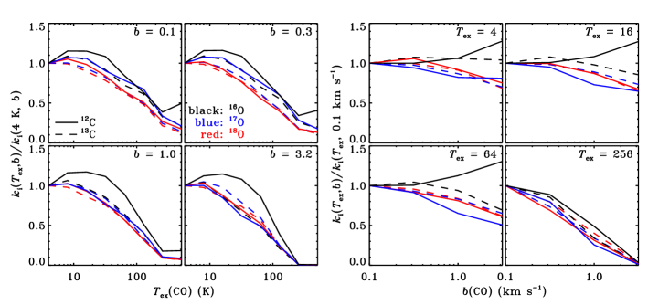
Figure 3: Left: photodissociation rate of the CO isotopologues as a function of excitation temperature, normalised to the rate at 4 K, at four different Doppler widths, for parameters corresponding to the centre of the $\zeta$ Oph diffuse cloud. Right: photodissociation rates as a function of Doppler width, normalised to the rate at 0.1 km s^-1, at four different excitation temperatures. The other model parameters are as in Sect. 3.3, except $b(\mathrm{H}_{2})=\sqrt{14}b(\mathrm{CO})$, $b(\mathrm{H})=\sqrt{28}b(\mathrm{CO})$ and $T_{\mathrm{ex}}(\mathrm{H}_{2})=[T_{\mathrm{ex}}(\mathrm{CO})]^{1.5}$.

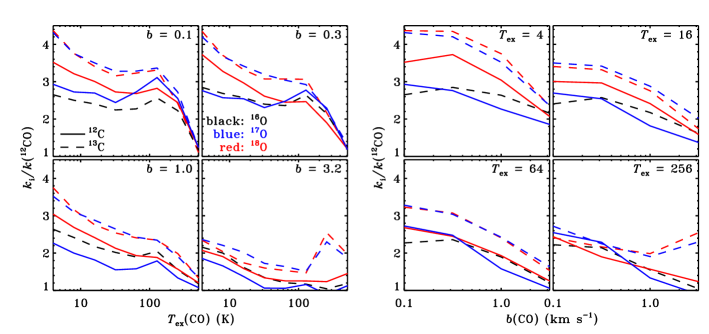
Figure 4: As Fig. 3, but with all rates normalised to the ¹²CO rate.

The left set of panels in Fig. 3 shows the photodissociation rate of the six isotopologues at the centre of the $\zeta$ Oph cloud as a function of excitation temperature for the different Doppler widths. The rates are normalised to the rate at 4 K. The ¹²CO rate increases from 4 to 16 K, as described in Sect. 4.1. At higher temperatures the increased overlap with H₂ lines takes over and the rate goes down. As long as the CO excitation temperature is less than $\sim$100 K, the ¹²CO rate remains constant up to $b(\mathrm{CO})=0.3$ km s^-1 and increases as $b(\mathrm{CO})$ goes from 0.3 to 3.2 km s^-1(right side of Fig. 3). At higher temperatures there is so much shielding by H₂ that reduced self-shielding in the CO lines has no discernable effect on the rate. Instead, the rate goes down with $b$ due to stronger shielding by the broadened H₂ lines.

The ¹³CO rate also increases initially with $T_{\mathrm{ex}}(\mathrm{CO})$ and then goes down as H₂ shielding takes over. The rate increases from $b(\mathrm{CO})=0.1$ to 0.3 km s^-1, but decreases for higher values as described in Sect. 4.2. For the remaining four isotopologues, the plotted curves likewise result from a combination of weaker shielding by ¹²CO and stronger shielding by H₂. At CO excitation temperatures between 4 and 8 K, the rates typically change by a few per cent either way. Going to higher temperatures, all rates decrease monotonically. Likewise, the rates generally decrease towards higher $b(\mathrm{CO})$ values.

A change in behaviour is seen when increasing $T_{\mathrm{ex}}(\mathrm{CO})$ from 256 to 512 K. It is at this point that the $v^{\prime\prime}$¿0 levels of H₂ become populated. Less energy is now needed to excite H₂ to the $B$ and $C$ states, so absorption shifts towards longer wavelengths. This causes even stronger shielding in the heavy CO isotopologues, for whom the $E0$ band at 1076 Å is still an important contributor to the photodissociation rate, at least as long as $b(\mathrm{CO})$ does not exceed 0.3 km s^-1. The $E0$ band is strongly self-shielded in ¹²CO (Table 4), so the shift of the H₂ absorption to longer wavelengths does not reduce its contribution by much. In fact, the weaker H₂ absorption at shorter wavelengths allows for an increased contribution of bands like Nos. 13 and 16 at 933 and 941 Å, causing a net increase in the ¹²CO photodissociation rate from 256 to 512 K. The situation changes somewhat when the CO Doppler width increases to 1.0 km s^-1 or more. The $E0$ band of the heavy isotopologues is now much less of a contributor, because it is shielded by the broader ¹²CO lines. The shifting H₂ absorption does not cause any additional shielding, so the rates remain almost the same. Furthermore, the H₂ lines are also broader and continue to shield the ¹²CO bands at shorter wavelengths, preventing its photodissociation rate from increasing like it does in the low-$b$ cases.

The main astrophysical consequence becomes clear when we look at the photodissociation rates of the five heavier isotopologues with respect to that of ¹²CO. Figure 4 shows this $k_{i}/k(^{12}\mathrm{CO})$ ratio as a function of $T_{\mathrm{ex}}(\mathrm{CO})$ and $b(\mathrm{CO})$. In these plots, the ¹²CO rate shows as a horizontal line with a value of unity. The ratios generally decrease with both parameters: a higher excitation temperature and a larger Doppler width both cause less self-shielding in ¹²CO, so the rate differences between the isotopologues become smaller. Shielding by H₂ increases at the same time, further reducing the differences between the isotopologues. This means that photodissociation of CO is more strongly isotope-selective in cold sources than in hot sources.

5 Shielding function approximations

It is unpractical for many astrophysical applications to do the full integration of all 5622 lines in our model every time a photodissociation rate is required. Therefore, we present approximations to the shielding functions $\Theta$ introduced in Eq. (2). The approximations are derived for several sets of model parameters and are valid across a wide range of astrophysical environments (Sect. 5.2).

5.1 Shielding functions on a two-dimensional grid of $N(\mathrm{CO})$ and $N(\mathrm{H}_{2})$

The transition from atomic to molecular hydrogen occurs much closer to the edge of the cloud than the $\@element[+]{\mathrm{C}}$–C–CO transition, so the column density of atomic H is roughly constant at the depths where shielding of CO is important. In addition, H shields CO by only a few per cent. Therefore, it is a good approximation to compute the shielding functions on a grid of CO and H₂ column densities, while taking a constant column of H. It is sufficient to express the shielding of all CO isotopologues as a function of $N(^{12}\mathrm{CO})$, because self-shielding of the heavier CO isotopologues is a small effect compared to shielding by ¹²CO.

Table 5: Two-dimensional shielding functions $\Theta[N(^{12}\mathrm{CO}),N(\mathrm{H}_{2})]$ for $b(\mathrm{CO})=0.3$ km s^-1, $T_{\mathrm{ex}}(\mathrm{CO})=5$ K and $N(^{12}\mathrm{CO})/N(^{13}\mathrm{CO})=69$.^a

$\log N(\mathrm{H}_{2})$	$\log{}^{12}\mathrm{CO}$ (cm-2)
(cm-2)	0	13	14	15	16	17	18	19
12CO: unattenuated rate $k_{0,i}=2.592\times 10^{-10}$ s-1
00	1.000(-0)	8.080(-1)	5.250(-1)	2.434(-1)	5.467(-2)	1.362(-2)	3.378(-3)	5.240(-4)
19	8.176(-1)	6.347(-1)	3.891(-1)	1.787(-1)	4.297(-2)	1.152(-2)	2.922(-3)	4.662(-4)
20	7.223(-1)	5.624(-1)	3.434(-1)	1.540(-1)	3.515(-2)	9.231(-3)	2.388(-3)	3.899(-4)
21	3.260(-1)	2.810(-1)	1.953(-1)	8.726(-2)	1.907(-2)	4.768(-3)	1.150(-3)	1.941(-4)
22	1.108(-2)	1.081(-2)	9.033(-3)	4.441(-3)	1.102(-3)	2.644(-4)	7.329(-5)	1.437(-5)
23	3.938(-7)	3.938(-7)	3.936(-7)	3.923(-7)	3.901(-7)	3.893(-7)	3.890(-7)	3.875(-7)
C17O: unattenuated rate $k_{0,i}=2.607\times 10^{-10}$ s-1
00	1.000(-0)	9.823(-1)	8.911(-1)	6.149(-1)	3.924(-1)	2.169(-1)	4.167(-2)	2.150(-3)
19	8.459(-1)	8.298(-1)	7.490(-1)	5.009(-1)	3.196(-1)	1.850(-1)	3.509(-2)	1.984(-3)
20	7.337(-1)	7.195(-1)	6.481(-1)	4.306(-1)	2.741(-1)	1.556(-1)	2.645(-2)	1.411(-3)
21	3.335(-1)	3.290(-1)	3.039(-1)	2.293(-1)	1.685(-1)	9.464(-2)	1.460(-2)	6.823(-4)
22	1.193(-2)	1.191(-2)	1.172(-2)	1.095(-2)	9.395(-3)	5.644(-3)	1.183(-3)	2.835(-5)
23	3.959(-7)	3.959(-7)	3.959(-7)	3.959(-7)	3.958(-7)	3.954(-7)	3.924(-7)	3.873(-7)
C18O: unattenuated rate $k_{0,i}=2.392\times 10^{-10}$ s-1
00	1.000(-0)	9.974(-1)	9.777(-1)	8.519(-1)	5.060(-1)	1.959(-1)	2.764(-2)	1.742(-3)
19	8.571(-1)	8.547(-1)	8.368(-1)	7.219(-1)	4.095(-1)	1.581(-1)	2.224(-2)	1.618(-3)
20	7.554(-1)	7.532(-1)	7.371(-1)	6.336(-1)	3.572(-1)	1.372(-1)	1.889(-2)	1.383(-3)
21	3.559(-1)	3.549(-1)	3.477(-1)	3.035(-1)	1.948(-1)	7.701(-2)	1.071(-2)	6.863(-4)
22	1.214(-2)	1.212(-2)	1.199(-2)	1.105(-2)	8.233(-3)	3.324(-3)	6.148(-4)	3.225(-5)
23	4.251(-7)	4.251(-7)	4.251(-7)	4.251(-7)	4.249(-7)	4.233(-7)	4.180(-7)	4.142(-7)
13CO: unattenuated rate $k_{0,i}=2.595\times 10^{-10}$ s-1
00	1.000(-0)	9.824(-1)	9.019(-1)	6.462(-1)	3.547(-1)	9.907(-2)	1.131(-2)	7.591(-4)
19	8.447(-1)	8.276(-1)	7.502(-1)	5.113(-1)	2.745(-1)	7.652(-2)	8.635(-3)	6.747(-4)
20	7.415(-1)	7.266(-1)	6.581(-1)	4.451(-1)	2.360(-1)	6.574(-2)	7.187(-3)	5.429(-4)
21	3.546(-1)	3.502(-1)	3.270(-1)	2.452(-1)	1.398(-1)	3.750(-2)	3.973(-3)	2.703(-4)
22	1.180(-2)	1.177(-2)	1.153(-2)	1.023(-2)	6.728(-3)	1.955(-3)	2.665(-4)	1.471(-5)
23	2.385(-7)	2.385(-7)	2.385(-7)	2.384(-7)	2.379(-7)	2.348(-7)	2.310(-7)	2.292(-7)
13C17O: unattenuated rate $k_{0,i}=2.598\times 10^{-10}$ s-1
00	1.000(-0)	9.979(-1)	9.820(-1)	8.832(-1)	5.942(-1)	3.177(-1)	1.523(-1)	3.885(-2)
19	8.540(-1)	8.520(-1)	8.374(-1)	7.469(-1)	4.901(-1)	2.677(-1)	1.302(-1)	3.135(-2)
20	7.405(-1)	7.387(-1)	7.254(-1)	6.439(-1)	4.198(-1)	2.333(-1)	1.142(-1)	2.607(-2)
21	3.502(-1)	3.494(-1)	3.434(-1)	3.076(-1)	2.214(-1)	1.386(-1)	6.941(-2)	1.195(-2)
22	1.279(-2)	1.278(-2)	1.267(-2)	1.198(-2)	1.045(-2)	7.743(-3)	4.088(-3)	4.581(-4)
23	2.370(-7)	2.370(-7)	2.370(-7)	2.370(-7)	2.369(-7)	2.368(-7)	2.359(-7)	2.312(-7)
13C18O: unattenuated rate $k_{0,i}=2.503\times 10^{-10}$ s-1
00	1.000(-0)	9.988(-1)	9.900(-1)	9.329(-1)	7.253(-1)	3.856(-1)	1.524(-1)	2.664(-2)
19	8.744(-1)	8.734(-1)	8.656(-1)	8.164(-1)	6.403(-1)	3.441(-1)	1.347(-1)	2.491(-2)
20	7.572(-1)	7.562(-1)	7.492(-1)	7.047(-1)	5.518(-1)	3.006(-1)	1.185(-1)	2.224(-2)
21	3.546(-1)	3.542(-1)	3.506(-1)	3.283(-1)	2.638(-1)	1.666(-1)	6.887(-2)	1.149(-2)
22	1.561(-2)	1.560(-2)	1.550(-2)	1.475(-2)	1.235(-2)	7.850(-3)	3.416(-3)	5.290(-4)
23	2.490(-7)	2.490(-7)	2.490(-7)	2.489(-7)	2.487(-7)	2.482(-7)	2.471(-7)	2.421(-7)

• These shielding functions were computed for the Draine (1978) radiation field ($\chi=1$) and the following set of parameters: $b(\mathrm{CO})=0.3$ km s^-1, $b(\mathrm{H}_{2})=3.0$ km s^-1 and $b(\mathrm{H})=5.0$ km s^-1; $T_{\mathrm{ex}}(\mathrm{CO})=5$ K and $T_{\mathrm{ex}}(\mathrm{H}_{2})=5^{1.5}$ K; $N(\mathrm{H})=5\times 10^{20}$ cm^-2; $N(^{12}\mathrm{CO})/N(^{13}\mathrm{CO})=69$, $N(^{12}\mathrm{CO})/N(\mathrm{C}^{18}\mathrm{O})=N(^{13}\mathrm{CO})/N(^{13}\mathrm{C}^{18}\mathrm{O})=557$ and $N(\mathrm{C}^{18}\mathrm{O})/N(\mathrm{C}^{17}\mathrm{O})=N(^{13}\mathrm{C}^{18}\mathrm{O})/N(^{13}\mathrm{C}^{17}\mathrm{O})=3.6$. Self-shielding is mostly negligible for the heavier isotopologues, so all shielding functions are expressed as a function of the ¹²CO column density. Continuum attenuation by dust is not included in this table (see Eq. (2)).

6

Table 6: As Table 5, for $b(\mathrm{CO})=0.3$ km s^-1, $T_{\mathrm{ex}}(\mathrm{CO})=50$ K and $N(^{12}\mathrm{CO})/N(^{13}\mathrm{CO})=69$.^a

$\log N(\mathrm{H}_{2})$	$\log{}^{12}\mathrm{CO}$ (cm-2)
(cm-2)	0	13	14	15	16	17	18	19
12CO: unattenuated rate $k_{0,i}=2.590\times 10^{-10}$ s-1
00	1.000(-0)	9.405(-1)	7.046(-1)	4.015(-1)	9.964(-2)	1.567(-2)	3.162(-3)	4.839(-4)
19	7.546(-1)	6.979(-1)	4.817(-1)	2.577(-1)	6.505(-2)	1.135(-2)	2.369(-3)	3.924(-4)
20	5.752(-1)	5.228(-1)	3.279(-1)	1.559(-1)	3.559(-2)	6.443(-3)	1.526(-3)	2.751(-4)
21	2.493(-1)	2.196(-1)	1.135(-1)	4.062(-2)	7.864(-3)	1.516(-3)	4.448(-4)	9.367(-5)
22	1.550(-3)	1.370(-3)	6.801(-4)	2.127(-4)	5.051(-5)	1.198(-5)	6.553(-6)	3.937(-6)
23	8.492(-8)	8.492(-8)	8.492(-8)	8.492(-8)	8.492(-8)	8.492(-8)	8.488(-8)	8.453(-8)
C17O: unattenuated rate $k_{0,i}=2.607\times 10^{-10}$ s-1
00	1.000(-0)	9.756(-1)	8.826(-1)	7.413(-1)	4.507(-1)	1.508(-1)	2.533(-2)	1.684(-3)
19	7.266(-1)	7.036(-1)	6.209(-1)	5.209(-1)	3.212(-1)	1.074(-1)	1.832(-2)	1.436(-3)
20	5.418(-1)	5.206(-1)	4.469(-1)	3.695(-1)	2.222(-1)	7.000(-2)	1.197(-2)	9.425(-4)
21	2.208(-1)	2.089(-1)	1.687(-1)	1.352(-1)	8.073(-2)	2.082(-2)	3.360(-3)	2.492(-4)
22	1.401(-3)	1.352(-3)	1.190(-3)	1.043(-3)	7.022(-4)	1.687(-4)	2.525(-5)	4.211(-6)
23	8.509(-8)	8.509(-8)	8.509(-8)	8.509(-8)	8.509(-8)	8.509(-8)	8.505(-8)	8.470(-8)
C18O: unattenuated rate $k_{0,i}=2.396\times 10^{-10}$ s-1
00	1.000(-0)	9.822(-1)	9.163(-1)	8.067(-1)	5.498(-1)	2.188(-1)	3.412(-2)	1.992(-3)
19	8.007(-1)	7.833(-1)	7.206(-1)	6.272(-1)	4.226(-1)	1.597(-1)	2.469(-2)	1.630(-3)
20	5.848(-1)	5.688(-1)	5.123(-1)	4.363(-1)	2.816(-1)	9.826(-2)	1.653(-2)	1.158(-3)
21	2.277(-1)	2.187(-1)	1.881(-1)	1.546(-1)	9.811(-2)	3.114(-2)	5.506(-3)	3.655(-4)
22	1.411(-3)	1.375(-3)	1.256(-3)	1.126(-3)	8.200(-4)	2.912(-4)	5.310(-5)	5.241(-6)
23	8.937(-8)	8.937(-8)	8.937(-8)	8.937(-8)	8.937(-8)	8.936(-8)	8.933(-8)	8.896(-8)
13CO: unattenuated rate $k_{0,i}=2.597\times 10^{-10}$ s-1
00	1.000(-0)	9.765(-1)	8.965(-1)	7.701(-1)	4.459(-1)	1.415(-1)	1.748(-2)	8.346(-4)
19	7.780(-1)	7.550(-1)	6.789(-1)	5.753(-1)	3.262(-1)	1.032(-1)	1.183(-2)	6.569(-4)
20	5.523(-1)	5.309(-1)	4.617(-1)	3.793(-1)	1.958(-1)	5.888(-2)	7.515(-3)	4.382(-4)
21	2.100(-1)	1.979(-1)	1.601(-1)	1.244(-1)	5.373(-2)	1.573(-2)	2.535(-3)	1.361(-4)
22	1.318(-3)	1.268(-3)	1.107(-3)	9.017(-4)	3.658(-4)	1.114(-4)	2.414(-5)	2.608(-6)
23	4.511(-8)	4.511(-8)	4.511(-8)	4.511(-8)	4.511(-8)	4.511(-8)	4.509(-8)	4.490(-8)
13C17O: unattenuated rate $k_{0,i}=2.605\times 10^{-10}$ s-1
00	1.000(-0)	9.853(-1)	9.344(-1)	8.453(-1)	5.978(-1)	3.075(-1)	1.180(-1)	3.205(-2)
19	8.097(-1)	7.954(-1)	7.474(-1)	6.755(-1)	4.947(-1)	2.711(-1)	1.065(-1)	2.898(-2)
20	5.925(-1)	5.792(-1)	5.363(-1)	4.815(-1)	3.576(-1)	2.062(-1)	8.289(-2)	1.967(-2)
21	2.389(-1)	2.315(-1)	2.083(-1)	1.848(-1)	1.410(-1)	8.627(-2)	3.185(-2)	3.489(-3)
22	1.937(-3)	1.907(-3)	1.812(-3)	1.711(-3)	1.474(-3)	1.042(-3)	3.690(-4)	1.704(-5)
23	4.523(-8)	4.523(-8)	4.523(-8)	4.523(-8)	4.523(-8)	4.523(-8)	4.521(-8)	4.502(-8)
13C18O: unattenuated rate $k_{0,i}=2.510\times 10^{-10}$ s-1
00	1.000(-0)	9.873(-1)	9.424(-1)	8.744(-1)	6.740(-1)	3.885(-1)	1.268(-1)	2.980(-2)
19	7.975(-1)	7.852(-1)	7.424(-1)	6.894(-1)	5.447(-1)	3.236(-1)	1.036(-1)	2.722(-2)
20	5.869(-1)	5.754(-1)	5.364(-1)	4.953(-1)	3.932(-1)	2.445(-1)	8.070(-2)	1.894(-2)
21	2.465(-1)	2.401(-1)	2.187(-1)	2.011(-1)	1.628(-1)	1.079(-1)	3.267(-2)	4.406(-3)
22	2.164(-3)	2.138(-3)	2.050(-3)	1.971(-3)	1.772(-3)	1.421(-3)	5.147(-4)	4.066(-5)
23	4.454(-8)	4.454(-8)	4.454(-8)	4.454(-8)	4.454(-8)	4.454(-8)	4.452(-8)	4.434(-8)

• These shielding functions were computed for the same parameters as in Table 5, except $T_{\mathrm{ex}}(\mathrm{CO})=50$ K and $T_{\mathrm{ex}}(\mathrm{H}_{2})=50^{1.5}$ K. Additional rotational lines of CO and H₂ were included as described in Sect. 4.4.

7

Table 7: As Table 5, for $b(\mathrm{CO})=3.0$ km s^-1, $T_{\mathrm{ex}}(\mathrm{CO})=5$ K and $N(^{12}\mathrm{CO})/N(^{13}\mathrm{CO})=69$.^a

$\log N(\mathrm{H}_{2})$	$\log{}^{12}\mathrm{CO}$ (cm-2)
(cm-2)	0	13	14	15	16	17	18	19
12CO: unattenuated rate $k_{0,i}=2.588\times 10^{-10}$ s-1
00	1.000(-0)	9.639(-1)	7.443(-1)	3.079(-1)	5.733(-2)	1.321(-2)	3.322(-3)	5.193(-4)
19	7.928(-1)	7.594(-1)	5.606(-1)	2.145(-1)	4.172(-2)	1.039(-2)	2.696(-3)	4.426(-4)
20	7.037(-1)	6.743(-1)	4.984(-1)	1.861(-1)	3.410(-2)	8.272(-3)	2.212(-3)	3.716(-4)
21	3.176(-1)	3.082(-1)	2.477(-1)	1.007(-1)	1.833(-2)	4.252(-3)	1.066(-3)	1.850(-4)
22	1.083(-2)	1.067(-2)	9.413(-3)	4.528(-3)	1.054(-3)	2.353(-4)	6.789(-5)	1.378(-5)
23	3.931(-7)	3.931(-7)	3.930(-7)	3.922(-7)	3.896(-7)	3.886(-7)	3.883(-7)	3.869(-7)
C17O: unattenuated rate $k_{0,i}=2.604\times 10^{-10}$ s-1
00	1.000(-0)	9.703(-1)	7.959(-1)	5.192(-1)	3.667(-1)	2.247(-1)	6.359(-2)	6.394(-3)
19	8.049(-1)	7.764(-1)	6.108(-1)	3.734(-1)	2.733(-1)	1.692(-1)	4.882(-2)	5.903(-3)
20	7.008(-1)	6.759(-1)	5.311(-1)	3.212(-1)	2.348(-1)	1.424(-1)	3.533(-2)	3.847(-3)
21	3.125(-1)	3.056(-1)	2.638(-1)	1.885(-1)	1.474(-1)	8.575(-2)	1.807(-2)	1.839(-3)
22	1.077(-2)	1.076(-2)	1.062(-2)	9.872(-3)	8.416(-3)	5.126(-3)	1.119(-3)	4.151(-5)
23	3.950(-7)	3.950(-7)	3.950(-7)	3.950(-7)	3.949(-7)	3.945(-7)	3.919(-7)	3.864(-7)
C18O: unattenuated rate $k_{0,i}=2.394\times 10^{-10}$ s-1
00	1.000(-0)	9.767(-1)	8.397(-1)	6.181(-1)	4.521(-1)	1.999(-1)	3.383(-2)	1.883(-3)
19	8.114(-1)	7.886(-1)	6.554(-1)	4.491(-1)	3.245(-1)	1.475(-1)	2.665(-2)	1.723(-3)
20	7.177(-1)	6.979(-1)	5.816(-1)	3.981(-1)	2.851(-1)	1.284(-1)	2.244(-2)	1.476(-3)
21	3.313(-1)	3.260(-1)	2.936(-1)	2.274(-1)	1.646(-1)	7.081(-2)	1.188(-2)	6.966(-4)
22	1.130(-2)	1.129(-2)	1.113(-2)	1.016(-2)	7.643(-3)	3.131(-3)	6.377(-4)	3.195(-5)
23	4.233(-7)	4.233(-7)	4.233(-7)	4.233(-7)	4.231(-7)	4.217(-7)	4.167(-7)	4.126(-7)
13CO: unattenuated rate $k_{0,i}=2.595\times 10^{-10}$ s-1
00	1.000(-0)	9.750(-1)	8.292(-1)	6.083(-1)	4.222(-1)	1.249(-1)	1.250(-2)	6.838(-4)
19	7.899(-1)	7.656(-1)	6.246(-1)	4.244(-1)	2.974(-1)	9.238(-2)	9.445(-3)	5.851(-4)
20	6.933(-1)	6.720(-1)	5.484(-1)	3.694(-1)	2.561(-1)	7.843(-2)	7.799(-3)	4.678(-4)
21	3.278(-1)	3.219(-1)	2.858(-1)	2.162(-1)	1.496(-1)	4.297(-2)	4.117(-3)	2.360(-4)
22	1.108(-2)	1.106(-2)	1.089(-2)	9.813(-3)	6.942(-3)	2.057(-3)	2.618(-4)	1.306(-5)
23	2.378(-7)	2.378(-7)	2.378(-7)	2.378(-7)	2.375(-7)	2.354(-7)	2.304(-7)	2.285(-7)
13C17O: unattenuated rate $k_{0,i}=2.604\times 10^{-10}$ s-1
00	1.000(-0)	9.800(-1)	8.605(-1)	6.553(-1)	5.067(-1)	2.970(-1)	1.491(-1)	4.514(-2)
19	8.134(-1)	7.939(-1)	6.781(-1)	4.891(-1)	3.826(-1)	2.401(-1)	1.228(-1)	3.233(-2)
20	7.049(-1)	6.879(-1)	5.867(-1)	4.192(-1)	3.270(-1)	2.096(-1)	1.079(-1)	2.669(-2)
21	3.302(-1)	3.256(-1)	2.970(-1)	2.382(-1)	1.931(-1)	1.292(-1)	6.607(-2)	1.136(-2)
22	1.174(-2)	1.173(-2)	1.161(-2)	1.093(-2)	9.517(-3)	7.132(-3)	3.652(-3)	3.436(-4)
23	2.312(-7)	2.312(-7)	2.312(-7)	2.312(-7)	2.311(-7)	2.311(-7)	2.308(-7)	2.290(-7)
13C18O: unattenuated rate $k_{0,i}=2.509\times 10^{-10}$ s-1
00	1.000(-0)	9.826(-1)	8.767(-1)	6.711(-1)	5.145(-1)	3.329(-1)	1.592(-1)	4.547(-2)
19	8.157(-1)	7.988(-1)	6.964(-1)	5.074(-1)	3.964(-1)	2.777(-1)	1.330(-1)	4.212(-2)
20	7.096(-1)	6.950(-1)	6.057(-1)	4.394(-1)	3.440(-1)	2.477(-1)	1.197(-1)	3.796(-2)
21	3.192(-1)	3.153(-1)	2.911(-1)	2.365(-1)	1.943(-1)	1.424(-1)	6.786(-2)	1.888(-2)
22	1.077(-2)	1.076(-2)	1.065(-2)	9.980(-3)	8.532(-3)	6.289(-3)	2.998(-3)	6.921(-4)
23	2.410(-7)	2.410(-7)	2.410(-7)	2.410(-7)	2.410(-7)	2.409(-7)	2.407(-7)	2.395(-7)

• These shielding functions were computed for the same parameters as in Table 5, except $b(\mathrm{CO})=3.0$ km s^-1, $b(\mathrm{H}_{2})=11.2$ km s^-1 and $b(\mathrm{H})=15.9$ km s^-1.

8

Table 8: As Table 5, for $b(\mathrm{CO})=0.3$ km s^-1, $T_{\mathrm{ex}}(\mathrm{CO})=5$ K and $N(^{12}\mathrm{CO})/N(^{13}\mathrm{CO})=35$.^a

$\log N(\mathrm{H}_{2})$	$\log{}^{12}\mathrm{CO}$ (cm-2)
(cm-2)	0	13	14	15	16	17	18	19
12CO: unattenuated rate $k_{0,i}=2.592\times 10^{-10}$ s-1
00	1.000(-0)	8.078(-1)	5.245(-1)	2.427(-1)	5.428(-2)	1.342(-2)	3.321(-3)	5.157(-4)
19	8.176(-1)	6.345(-1)	3.886(-1)	1.781(-1)	4.271(-2)	1.136(-2)	2.875(-3)	4.591(-4)
20	7.223(-1)	5.623(-1)	3.430(-1)	1.534(-1)	3.493(-2)	9.095(-3)	2.347(-3)	3.842(-4)
21	3.260(-1)	2.810(-1)	1.951(-1)	8.696(-2)	1.894(-2)	4.691(-3)	1.127(-3)	1.913(-4)
22	1.108(-2)	1.081(-2)	9.030(-3)	4.434(-3)	1.096(-3)	2.606(-4)	7.208(-5)	1.420(-5)
23	3.938(-7)	3.938(-7)	3.936(-7)	3.923(-7)	3.901(-7)	3.893(-7)	3.890(-7)	3.875(-7)
C17O: unattenuated rate $k_{0,i}=2.607\times 10^{-10}$ s-1
00	1.000(-0)	9.791(-1)	8.675(-1)	5.829(-1)	3.848(-1)	2.122(-1)	4.089(-2)	2.102(-3)
19	8.459(-1)	8.266(-1)	7.258(-1)	4.699(-1)	3.139(-1)	1.810(-1)	3.440(-2)	1.941(-3)
20	7.337(-1)	7.168(-1)	6.280(-1)	4.036(-1)	2.691(-1)	1.518(-1)	2.583(-2)	1.378(-3)
21	3.335(-1)	3.283(-1)	2.988(-1)	2.218(-1)	1.655(-1)	9.193(-2)	1.417(-2)	6.647(-4)
22	1.193(-2)	1.191(-2)	1.171(-2)	1.091(-2)	9.219(-3)	5.456(-3)	1.149(-3)	2.666(-5)
23	3.959(-7)	3.959(-7)	3.959(-7)	3.959(-7)	3.958(-7)	3.954(-7)	3.923(-7)	3.873(-7)
C18O: unattenuated rate $k_{0,i}=2.392\times 10^{-10}$ s-1
00	1.000(-0)	9.971(-1)	9.757(-1)	8.410(-1)	4.805(-1)	1.677(-1)	2.310(-2)	1.529(-3)
19	8.571(-1)	8.544(-1)	8.349(-1)	7.120(-1)	3.881(-1)	1.349(-1)	1.861(-2)	1.421(-3)
20	7.554(-1)	7.531(-1)	7.353(-1)	6.247(-1)	3.379(-1)	1.166(-1)	1.562(-2)	1.212(-3)
21	3.559(-1)	3.549(-1)	3.470(-1)	2.995(-1)	1.827(-1)	6.493(-2)	8.710(-3)	5.900(-4)
22	1.214(-2)	1.212(-2)	1.197(-2)	1.091(-2)	7.560(-3)	2.781(-3)	4.965(-4)	2.789(-5)
23	4.251(-7)	4.251(-7)	4.251(-7)	4.251(-7)	4.248(-7)	4.228(-7)	4.175(-7)	4.141(-7)
13CO: unattenuated rate $k_{0,i}=2.595\times 10^{-10}$ s-1
00	1.000(-0)	9.788(-1)	8.746(-1)	5.882(-1)	2.889(-1)	6.582(-2)	7.841(-3)	6.070(-4)
19	8.447(-1)	8.241(-1)	7.241(-1)	4.601(-1)	2.237(-1)	5.052(-2)	6.312(-3)	5.444(-4)
20	7.415(-1)	7.235(-1)	6.353(-1)	4.000(-1)	1.921(-1)	4.324(-2)	5.236(-3)	4.396(-4)
21	3.546(-1)	3.494(-1)	3.205(-1)	2.277(-1)	1.138(-1)	2.454(-2)	2.807(-3)	2.164(-4)
22	1.180(-2)	1.176(-2)	1.148(-2)	9.874(-3)	5.564(-3)	1.339(-3)	1.818(-4)	1.270(-5)
23	2.385(-7)	2.385(-7)	2.384(-7)	2.383(-7)	2.374(-7)	2.335(-7)	2.306(-7)	2.292(-7)
13C17O: unattenuated rate $k_{0,i}=2.598\times 10^{-10}$ s-1
00	1.000(-0)	9.977(-1)	9.803(-1)	8.723(-1)	5.661(-1)	2.965(-1)	1.436(-1)	3.191(-2)
19	8.540(-1)	8.519(-1)	8.359(-1)	7.377(-1)	4.699(-1)	2.518(-1)	1.236(-1)	2.638(-2)
20	7.405(-1)	7.385(-1)	7.241(-1)	6.360(-1)	4.035(-1)	2.204(-1)	1.084(-1)	2.199(-2)
21	3.502(-1)	3.494(-1)	3.428(-1)	3.038(-1)	2.130(-1)	1.330(-1)	6.616(-2)	1.008(-2)
22	1.279(-2)	1.278(-2)	1.267(-2)	1.193(-2)	1.021(-2)	7.576(-3)	3.904(-3)	3.924(-4)
23	2.370(-7)	2.370(-7)	2.370(-7)	2.370(-7)	2.369(-7)	2.368(-7)	2.358(-7)	2.311(-7)
13C18O: unattenuated rate $k_{0,i}=2.503\times 10^{-10}$ s-1
00	1.000(-0)	9.988(-1)	9.893(-1)	9.277(-1)	7.041(-1)	3.637(-1)	1.353(-1)	1.838(-2)
19	8.744(-1)	8.734(-1)	8.652(-1)	8.132(-1)	6.262(-1)	3.264(-1)	1.205(-1)	1.727(-2)
20	7.572(-1)	7.562(-1)	7.488(-1)	7.022(-1)	5.411(-1)	2.868(-1)	1.064(-1)	1.546(-2)
21	3.546(-1)	3.541(-1)	3.504(-1)	3.272(-1)	2.592(-1)	1.608(-1)	6.195(-2)	7.985(-3)
22	1.561(-2)	1.560(-2)	1.550(-2)	1.471(-2)	1.214(-2)	7.623(-3)	3.112(-3)	3.736(-4)
23	2.490(-7)	2.490(-7)	2.490(-7)	2.489(-7)	2.487(-7)	2.482(-7)	2.470(-7)	2.419(-7)

• These shielding functions were computed for the same parameters as in Table 5, except $N(^{12}\mathrm{CO})/N(^{13}\mathrm{CO})=35$.

Table 5 presents the shielding functions in the same manner as vDB88 did, but for somewhat different model parameters: $b(\mathrm{CO})=0.3$ instead of 1.0 km s^-1, $T_{\mathrm{ex}}(\mathrm{CO})=5$ instead of 10 K, and $T_{\mathrm{ex}}(\mathrm{H}_{2})=5^{1.5}$ instead of $10^{1.5}$ K. The present parameters correspond more closely to what is observed in diffuse and translucent clouds. The column density ratios for the six isotopologues are kept constant at the elemental isotope ratios from Wilson (1999): $[\@element[12]{\mathrm{C}}]/[\@element[13]{\mathrm{C}}]=69$, $[\@element[16]{\mathrm{O}}]/[\@element[18]{\mathrm{O}}]=557$ and $[\@element[18]{\mathrm{O}}]/[\@element[17]{\mathrm{O}}]=3.6$. A small column of $5.2\times 10^{15}$ cm^-2 of H₂ at $J^{\prime\prime}$=4–7 is included throughout (except at $\log N(\mathrm{H}_{2})=0$) to account for UV pumping (Sect. 3.1). Shielding functions for larger values of $b$ and $T_{\mathrm{ex}}$ and for other isotope ratios are given in Tables 6–8 in the online appendix to this paper. For ease of use, we have also set up a webpage where the shielding functions can be downloaded in plain text format. This webpage offers shielding functions for a wider variety of parameters than is possible to include in this paper. In addition, it uses a grid of $N(^{12}\mathrm{CO}$) and $N(\mathrm{H}_{2})$ values that is five times finer than the grid in Tables 5–8, allowing for more accurate interpolation.

For column densities of up to $10^{17}$ cm^-2 of CO and $10^{21}$ cm^-2 of H₂, our shielding functions are generally within a few per cent of the vDB88 values when corrected for the difference in $b$ and $T_{\mathrm{ex}}$. Larger differences occur for larger columns: we predict the shielding to be about five times weaker at $N(\mathrm{CO})=10^{19}$ cm^-2 and more than a hundred times stronger at $N(\mathrm{H}_{2})=10^{23}$ cm^-2. The 912-1118 Å wavelength range was divided into 23 bins by vDB88, and most lines were included only in one bin to speed up the computation. We integrate all lines over all wavelengths. As the lines get strongly saturated at high column depths, absorption in the line wings becomes important. Thus, H₂ lines can cause substantial shielding over a range of more than 10 Å, while CO lines may still absorb several Å away from the line centre. The binned integration method of vDB88 did not take these effects into account, so they underpredicted shielding at large H₂ columns and overpredicted shielding at large CO columns (Fig. 5). It should be noted, however, that photodissociation at these depths is typically already so slow a process that it is no longer the dominant destruction pathway for CO. In addition, a large CO column is usually accompanied by a large H₂ column, so the two effects partially cancel each other.

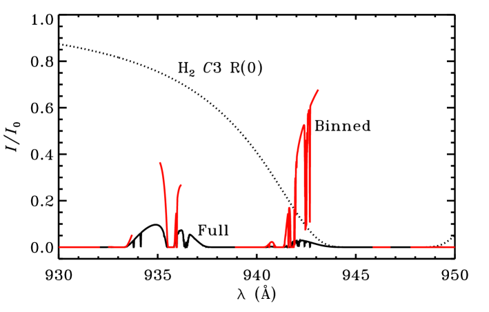
Figure 5: Illustration of the effect of not integrating strongly saturated lines over the entire wavelength regime. Full black curve: relative intensity of the radiation field at $N(\mathrm{CO})=10^{18}$ and $N(\mathrm{H}_{2})=10^{22}$ cm^-2 for the parameters of Table 5, computed with a full integration of all lines over all wavelengths. Red curve: the same, but computed with the binned integration method of vDB88. Dotted curve: attenuation due to the $C3$ R(0) line of H₂, centred on 946.42 Å. This line was not included by vDB88 when computing the shielding in the 938.9–943.1 Å bin, thus overestimating the photodissociation rate in the $W2$ band at 941.1 Å.

5.2 Comparison between the full model and the approximations

Despite being computed for a limited number of model parameters, the shielding functions from Tables 5–8 provide a good approximation to the rates from the full model for a wide range of astrophysical environments. Section 6.1 presents a grid of translucent cloud models, where the photodissociation model is coupled to a chemical network and CO is traced as a function of depth. This presents a large range of column densities, with the ratios between the isotopologues deviating from the fixed values adopted for Tables 5–8. The grid covers gas densities from 100 to 1000 cm^-3 and gas temperatures from 15 to 100 K, while keeping the excitation temperatures and Doppler widths constant at the values used for Table 5. Altogether, the grid contains 2880 points per isotopologue where the photodissociation rate is computed. Here, we compare the photodissociaton rates from the approximate method to the full integration for each of these points. The sensitivity of $k(^{13}\mathrm{CO})$ to the $N(^{12}\mathrm{CO})/N(^{13}\mathrm{CO})$ ratio can be corrected for in a simple manner: we use the shielding functions from Table 8 when the ratio is closer to 35 than to 69, and those from Table 5 otherwise.

The rate from our approximate method is within 10% of the “real” rate in 98.3% of all points (Fig. 6). In no cases is the difference between the approximate rates and the full model more than 40%. Perhaps even more important than the absolute photodissociation rates are the ratios, $Q$, between the rates of ¹²CO and the other five isotopologues ^xC^yO:

$$Q_{i}=\frac{k(^{x}\mathrm{C}^{y}\mathrm{O})}{k(^{12}\mathrm{CO})}\,.$$ (3)

The shielding functions from Tables 5 and 8 together reproduce the ratios from the full method to the same accuracy as the absolute rates. At 98.4% of all points in the grid of translucent clouds, the ratios are off by less than 10% (Fig. 6). Similar scores can be obtained for models of PDRs or other environments if one uses shielding functions computed for the right combination of parameters. Otherwise, the accuracy goes down. For example, the shielding functions from Table 5 ($T_{\mathrm{ex}}(\mathrm{CO})=5$ K) can easily give photodissociation rates off by a factor of two when applied to a high-density, high-temperature PDR.

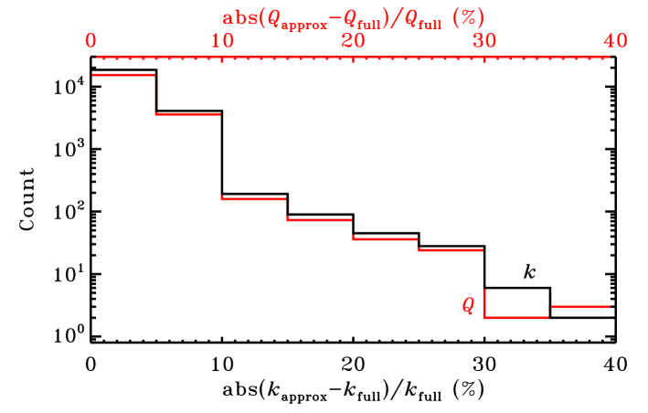
Figure 6: Histogram of the absolute relative difference between the approximate method (Tables 5 and 8; see text for details) and the full computation for the absolute photodissociation rates ($k$, black line) and the isotopologue rate ratios ($Q$, red line) in a grid of translucent cloud models. The data for all six isotopologues are taken together, but the $Q$ values for ¹²CO (which are unity regardless of the method) are omitted.

6 Chemistry of CO: astrophysical implications

Photodissociation is an important destruction mechanism for CO in many environments. In this section, we couple the photodissociation model to a small chemical network in order to explore abundances and column densities. Specifically, we model the CO chemistry in translucent clouds, PDRs and circumstellar disks, and we compare our results to observations of such objects. The photodissociation rates are computed with our full model throughout this section.

6.1 Translucent clouds

6.1.1 Model setup

Translucent clouds, with visual extinctions between 1 and 5 mag, form an excellent test case for our CO photodissociation model. Two recent studies of several dozen lines of sight through diffuse ($A_{\mathrm{V}}<1$ mag) and translucent clouds provide a set of CO and H₂ column densities for comparison (Sonnentrucker et al. 2007; Sheffer et al. 2008). These surveys show a clear correlation between $N(\mathrm{H}_{2})$ and $N(^{12}\mathrm{CO})$, with distinctly different slopes for H₂ columns of less and more than $2.5\times 10^{20}$ cm^-2. Sheffer et al. attributed this break to a change in the formation mechanism of CO. Their models show that the two-step conversion from $\@element[+]{\mathrm{C}}$ to CH⁺ and CO⁺,

$$\@element[+]{\mathrm{C}}\ +\ \mathrm{H}_{2}\ \to\ \mathrm{CH}^{+}\ +\ \@element{\mathrm{H}}\,,$$ (4)

$$\mathrm{CH}^{+}\ +\ \@element{\mathrm{O}}\ \to\ \@element{\mathrm{CO}}^{+}\ +\ \@element{\mathrm{H}}\,,$$ (5)

followed by reaction with H (forming CO directly) or H₂ (forming HCO⁺, which then recombines with an electron to give CO) is the dominant pathway at low column densities. However, the highly endothermic Reaction (4) is not fast enough at gas kinetic temperatures typical for these environments to explain the observed abundances of CH⁺ and CO. Suprathermal chemistry has been suggested as a solution to this problem. Sheffer et al. followed the approach of Federman et al. (1996), who argued that Alfvén waves entering the cloud from the outside result in non-thermal motions between ions and neutrals. Other mechanisms have been suggested by Joulain et al. (1998) and Pety & Falgarone (2000). The effect of the Alfvén waves can be incorporated into a chemical model by replacing the kinetic temperature in the rate equation for Reaction (4) and all other ion-neutral reactions by an effective temperature:

$$T_{\mathrm{eff}}=T_{\mathrm{gas}}+\frac{\mu v_{\mathrm{A}}^{2}}{3k_{\mathrm{B}}}\,.$$ (6)

Here, $k_{\mathrm{B}}$ is the Boltzmann constant, $\mu$ is the reduced mass of the reactants and $v_{\mathrm{A}}$ is the Alfvén speed. The Alfvén waves reach a depth of a few $10^{20}$ cm^-2 of H₂, corresponding to an $A_{\mathrm{V}}$ of a few tenths of a magnitude, beyond which suprathermal chemistry ceases to be important. CO can therefore no longer be formed efficiently through Reactions (4) and (5), and the reaction between $\@element[+]{\mathrm{C}}$ and OH (producing CO either directly or via a CO⁺ intermediate) takes over as the key route to CO. The identification of these two different chemistry regimes supports the conclusion of Zsargó & Federman (2003) that suprathermal chemistry is required to explain observed CO abundances in diffuse environments. Suprathermal chemistry also drives up the HCO⁺ abundance, confirming the conclusion of Liszt & Lucas (1994) and Liszt (2007) that HCO⁺ is the dominant precursor to CO in diffuse clouds.

We present here a grid of translucent cloud models to see how well the new photodissociation results match the observations. We set the Alfvén speed to 3.3 km s^-1 for $N(\mathrm{H}_{2})<4\times 10^{20}$ cm^-2 and to zero for larger column densities (Sheffer et al. 2008). The grid comprises densities ($n_{\mathrm{H}}=n(\mathrm{H})+2n(\mathrm{H}_{2})$) of 100, 300, 500, 700 and 1000 cm^-3, gas temperatures of 15, 30, 50 and 100 K, and relative UV intensities ($\chi$) of 1, 3 and 10. The dust temperature is assumed to stay low for all models ($\sim 15$ K), so the H₂ formation rate does not change. The ionisation rate of H due to cosmic rays is set to a constant value of $1.3\times 10^{-17}$ s^-1. Attenuation by 0.1 $\mu$m dust grains (Sect. 3.4) is taken into account. The Doppler widths and level populations are as described in Sect. 3.1, with CO and H₂ excitation temperatures of 5 and $5^{1.5}$ K. Taking other $b$ or $T_{\mathrm{ex}}$ values plausible for these environments does not alter our results significantly. All models are run to an $A_{\mathrm{V}}$ of 5 mag; results are also presented for a range of smaller extinctions.

The models require a chemical network to compute the abundances at each depth step. Since we are only interested in CO, the number of relevant species and reactions is limited. We adopt the network from a recent PDR benchmark study (Röllig et al. 2007), which includes only 31 species consisting of H, He, C and O. We duplicate all C- and O-containing species and reactions for $\@element[13]{\mathrm{C}}$, $\@element[17]{\mathrm{O}}$ and $\@element[18]{\mathrm{O}}$. Freeze-out and thermal evaporation are added for all neutral species, but no grain-surface reactions are included other than H₂ formation according to Black & van Dishoeck (1987). We add ion-molecule exchange reactions such as

$$^{12}\mathrm{CO}\ +\ \@element[+][13]{\mathrm{C}}\ \rightleftarrows\ \@element[+][12]{\mathrm{C}}\ +\ ^{13}\mathrm{CO}\ +\ 35\ \mathrm{K}\,,$$ (7)

$$\mathrm{H}^{12}\mathrm{CO}^{+}\ +\ ^{13}\mathrm{CO}\ \rightleftarrows\ ^{12}\mathrm{CO}\ +\ \mathrm{H}^{13}\mathrm{CO}^{+}\ +\ 9\ \mathrm{K}\,,$$ (8)

which can enhance the abundances of the heavy isotopologues of CO and HCO⁺ (Watson et al. 1976; Smith & Adams 1980; Langer et al. 1984). The temperature-dependence of the rate of these two reactions was fitted by Liszt (2007); the alternative equations from Woods & Willacy (2009) give the same results. The effective temperature from Eq. (6) is used instead of the kinetic temperature for all ion-neutral reactions, including Reactions (7) and (8). Altogether, the network contains 118 species and 1723 reactions. We adopt the elemental abundances of Cardelli et al. (1996) and isotope ratios appropriate for the local ISM ($[\@element[12]{\mathrm{C}}]/[\@element[13]{\mathrm{C}}]=69$, $[\@element[16]{\mathrm{O}}]/[\@element[18]{\mathrm{O}}]=557$ and $[\@element[18]{\mathrm{O}}]/[\@element[17]{\mathrm{O}}]=3.6$; Wilson 1999); the complete list of elemental abundances is given in Table 9. Chemical steady state is reached at all depths after $\sim$1 Myr, regardless of whether the gas starts in atomic or molecular form.

Table 9: Elemental abundances.

Element	Abundance relative to $n_{\mathrm{H}}$
He	$1.00\times 10^{-1}$
$\@element[12]{\mathrm{C}}$	$1.40\times 10^{-4}$
$\@element[13]{\mathrm{C}}$	$2.03\times 10^{-6}$
$\@element[16]{\mathrm{O}}$	$3.10\times 10^{-4}$
$\@element[17]{\mathrm{O}}$	$1.55\times 10^{-7}$
$\@element[18]{\mathrm{O}}$	$5.57\times 10^{-7}$

6.1.2 ¹²CO

The left panel of Fig. 7 shows $N(^{12}\mathrm{CO})$ versus $N(\mathrm{H}_{2})$ for all depth steps in our grid. These and other column densities are also listed for a set of selected $A_{\mathrm{V}}$ values in Tables 10–13 in the online appendix to this paper. The scatter in the data is due to the different physical parameters. For a given $N(\mathrm{H}_{2})$, $N(^{12}\mathrm{CO})$ is about two times larger at $T_{\mathrm{gas}}=100$ K than at 15 K. The formation rate of H₂ increases with temperature; through the chain of reactions starting with Reaction (4), that results in a larger CO abundance and column density. Up to $N(\mathrm{H}_{2})=10^{21}$ cm^-2, increasing the gas density by a factor of ten increases $N(^{12}\mathrm{CO})/N(\mathrm{H}_{2})$ also by about a factor of ten. This is due to the photodissociation rate being mostly independent of density, while the rates of the two-body reactions forming CO are not. Photodissociation ceases to be the main destruction mechanism for CO deeper into the cloud, so increasing $n_{\mathrm{H}}$ has a smaller effect there. Increasing the UV intensity from $\chi=1$ to 10 has the simple effect of decreasing $N(^{12}\mathrm{CO})/N(\mathrm{H}_{2})$ roughly tenfold for $N(\mathrm{H}_{2})<10^{21}$ cm^-2. For larger depths, changing $\chi$ only has a small effect. These dependencies on the physical parameters are consistent with the observations of Sheffer et al. (2008).

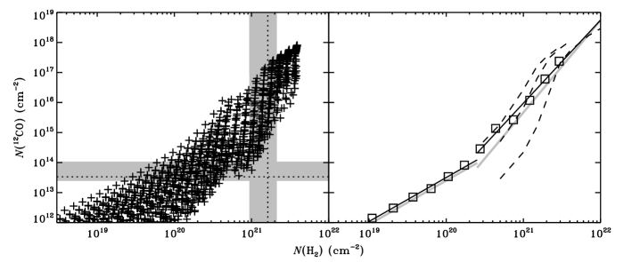
Figure 7: Column densities of ¹²CO versus those of H₂. Left: data for all points with $A_{\mathrm{V}}\leq 5$ mag from our grid of translucent cloud models, covering $n_{\mathrm{H}}=100$–1000 cm^-3, $T_{\mathrm{gas}}=15$–100 K and $\chi=1$–10. The vertical grey band indicates the range over which photodissociation ceases to be the dominant destruction mechanism of ¹²CO; the dotted line is the median. Likewise, the horizontal band indicates the range over which ¹²CO becomes self-shielding. Right: 100-point means of our model results (black squares), fitted with two straight lines. Also shown are the fits to the observations by Sheffer et al. (2008, grey lines) and the results from the translucent cloud models of vDB88 (dashed lines) for $\chi=0.5$, 1 and 10 (left to right).

Figure 8: Column densities of ¹³CO (left) and column density ratios of ¹²CO to ¹³CO (right) plotted against the column density of H₂. Grey crosses: observations of Sonnentrucker et al. (2007), Burgh et al. (2007) and Sheffer et al. (2007). Black squares and straight lines: 100-point means from our grid of translucent cloud models, offset by a factor of three in the right panel. Dotted line: median depth at which ¹²CO becomes self-shielding. Black plus signs: model data for all points with $A_{\mathrm{V}}\leq 5$ mag. Dashed lines: data from the translucent cloud models of vDB88 for $\chi=0.5$, 1 and 10 (left to right).

10

Table 10: Column densities (in cm^-2) for our grid of translucent cloud models at $T_{\mathrm{gas}}=15$ K. Results for $n_{\mathrm{H}}=500$ and 700 cm^-3 are not shown.

Model	$n_{\mathrm{H}}$	$\chi$	$A_{\mathrm{V}}$	$N(\mathrm{H}_{2})$	$N(\mathrm{H})$	$N(^{12}\mathrm{CO})$	$N(\mathrm{C}^{17}\mathrm{O})$	$N(\mathrm{C}^{18}\mathrm{O})$	$N(^{13}\mathrm{CO})$	$N(^{13}\mathrm{C}^{17}\mathrm{O})$	$N(^{13}\mathrm{C}^{18}\mathrm{O})$
	(cm-3)		(mag)
A1$\alpha$	0100	01	0.08	1.0(19)	1.1(20)	1.1(11)	5.2(7)0	2.0(8)0	1.5(9)0	7.7(5)0	2.8(6)0
			0.14	3.0(19)	1.7(20)	4.6(11)	2.2(8)0	8.5(8)0	6.7(9)0	3.3(6)0	1.2(7)0
			0.30	1.0(20)	2.8(20)	3.1(12)	1.4(9)0	5.5(9)0	4.4(10)	2.2(7)0	8.1(7)0
			0.71	3.0(20)	5.1(20)	4.5(13)	1.7(10)	6.4(10)	5.2(11)	2.5(8)0	9.2(8)0
			1.70	1.0(21)	6.8(20)	4.3(14)	1.3(11)	4.6(11)	1.6(13)	5.4(9)0	1.8(10)
			4.20	3.0(21)	6.9(20)	1.6(16)	7.4(12)	2.6(13)	1.4(15)	6.6(11)	2.4(12)
A1$\beta$	0100	03	0.20	1.0(19)	2.9(20)	2.7(10)	1.3(7)0	5.0(7)0	3.9(8)0	1.9(5)0	7.0(5)0
			0.29	3.0(19)	3.9(20)	1.3(11)	6.1(7)0	2.4(8)0	1.9(9)0	9.2(5)0	3.4(6)0
			0.48	1.0(20)	5.5(20)	1.0(12)	4.9(8)0	1.9(9)0	1.5(10)	7.5(6)0	2.7(7)0
			0.90	3.0(20)	8.2(20)	1.6(13)	7.0(9)0	2.6(10)	2.1(11)	1.0(8)0	3.8(8)0
			1.90	1.0(21)	1.0(21)	1.9(14)	6.4(10)	2.3(11)	6.2(12)	2.2(9)0	8.0(9)0
			4.50	3.0(21)	1.0(21)	1.1(16)	5.0(12)	1.8(13)	9.7(14)	4.7(11)	1.7(12)
A1$\gamma$	0100	10	0.46	1.0(19)	7.0(20)	1.2(10)	5.5(6)0	2.1(7)0	1.6(8)0	8.1(4)0	3.0(5)0
			0.59	3.0(19)	8.7(20)	6.1(10)	2.9(7)0	1.1(8)0	8.9(8)0	4.4(5)0	1.6(6)0
			0.81	1.0(20)	1.1(21)	5.7(11)	2.7(8)0	1.1(9)0	8.5(9)0	4.2(6)0	1.5(7)0
			1.20	3.0(20)	1.4(21)	9.6(12)	4.4(9)0	1.7(10)	1.4(11)	6.7(7)0	2.4(8)0
			2.30	1.0(21)	1.6(21)	1.0(14)	3.9(10)	1.4(11)	3.4(12)	1.3(9)0	4.9(9)0
			4.80	3.0(21)	1.6(21)	7.3(15)	3.5(12)	1.3(13)	7.1(14)	3.5(11)	1.3(12)
A2$\alpha$	0300	01	0.04	1.0(19)	4.4(19)	4.3(11)	2.1(8)0	8.0(8)0	6.2(9)0	3.1(6)0	1.1(7)0
			0.09	3.0(19)	7.5(19)	1.8(12)	8.7(8)0	3.4(9)0	2.7(10)	1.3(7)0	4.9(7)0
			0.23	1.0(20)	1.6(20)	1.2(13)	5.2(9)0	2.0(10)	1.6(11)	7.8(7)0	2.9(8)0
			0.60	3.0(20)	3.5(20)	1.7(14)	5.3(10)	1.9(11)	1.6(12)	7.4(8)0	2.7(9)0
			1.50	1.0(21)	4.5(20)	1.4(15)	3.6(11)	1.1(12)	8.1(13)	2.1(10)	6.6(10)
			4.10	3.0(21)	4.5(20)	1.5(17)	6.8(13)	2.5(14)	2.8(15)	1.1(12)	4.2(12)
A2$\beta$	0300	03	0.08	1.0(19)	1.1(20)	7.8(10)	3.7(7)0	1.4(8)0	1.1(9)0	5.6(5)0	2.1(6)0
			0.14	3.0(19)	1.7(20)	3.7(11)	1.8(8)0	6.8(8)0	5.4(9)0	2.7(6)0	9.9(6)0
			0.30	1.0(20)	2.8(20)	2.7(12)	1.3(9)0	4.8(9)0	3.9(10)	1.9(7)0	7.1(7)0
			0.70	3.0(20)	5.1(20)	3.9(13)	1.5(10)	5.7(10)	4.7(11)	2.3(8)0	8.3(8)0
			1.70	1.0(21)	6.7(20)	4.3(14)	1.3(11)	4.5(11)	1.9(13)	5.9(9)0	2.0(10)
			4.20	3.0(21)	6.8(20)	9.8(16)	4.3(13)	1.5(14)	2.3(15)	9.8(11)	3.6(12)
A2$\gamma$	0300	10	0.21	1.0(19)	3.2(20)	1.9(10)	8.9(6)0	3.4(7)0	2.7(8)0	1.3(5)0	4.8(5)0
			0.30	3.0(19)	4.2(20)	9.3(10)	4.5(7)0	1.7(8)0	1.4(9)0	6.8(5)0	2.5(6)0
			0.50	1.0(20)	5.9(20)	8.3(11)	4.0(8)0	1.5(9)0	1.2(10)	6.1(6)0	2.2(7)0
			0.92	3.0(20)	8.6(20)	1.4(13)	6.0(9)0	2.3(10)	1.8(11)	9.0(7)0	3.3(8)0
			1.90	1.0(21)	1.1(21)	1.5(14)	5.2(10)	1.9(11)	5.4(12)	1.9(9)0	7.0(9)0
			4.50	3.0(21)	1.1(21)	6.5(16)	2.9(13)	1.1(14)	2.0(15)	8.6(11)	3.2(12)
A5$\alpha$	1000	01	0.02	1.0(19)	1.9(19)	2.5(12)	1.1(9)0	4.5(9)0	3.5(10)	1.7(7)0	6.5(7)0
			0.06	3.0(19)	4.0(19)	1.0(13)	4.4(9)0	1.7(10)	1.4(11)	6.8(7)0	2.5(8)0
			0.19	1.0(20)	1.0(20)	6.9(13)	2.4(10)	8.8(10)	7.4(11)	3.5(8)0	1.3(9)0
			0.53	3.0(20)	2.4(20)	9.0(14)	2.2(11)	7.0(11)	7.2(12)	2.8(9)0	1.0(10)
			1.50	1.0(21)	3.0(20)	1.4(16)	1.9(12)	5.6(12)	2.4(14)	3.4(10)	1.1(11)
			4.00	3.0(21)	3.0(20)	5.9(16)	2.1(13)	7.3(13)	8.8(14)	3.0(11)	1.1(12)
A5$\beta$	1000	03	0.04	1.0(19)	4.0(19)	4.5(11)	2.1(8)0	8.3(8)0	6.6(9)0	3.3(6)0	1.2(7)0
			0.08	3.0(19)	7.0(19)	2.0(12)	9.3(8)0	3.6(9)0	2.9(10)	1.4(7)0	5.3(7)0
			0.22	1.0(20)	1.5(20)	1.3(13)	5.6(9)0	2.1(10)	1.7(11)	8.5(7)0	3.1(8)0
			0.60	3.0(20)	3.4(20)	1.8(14)	5.6(10)	2.0(11)	1.7(12)	8.0(8)0	2.9(9)0
			1.50	1.0(21)	4.3(20)	1.8(15)	4.5(11)	1.4(12)	9.3(13)	2.2(10)	6.7(10)
			4.10	3.0(21)	4.3(20)	4.7(16)	1.8(13)	6.4(13)	7.7(14)	2.8(11)	9.8(11)
A5$\gamma$	1000	10	0.08	1.0(19)	1.1(20)	6.7(10)	3.2(7)0	1.2(8)0	9.8(8)0	4.8(5)0	1.8(6)0
			0.14	3.0(19)	1.7(20)	3.4(11)	1.6(8)0	6.3(8)0	5.0(9)0	2.5(6)0	9.1(6)0
			0.30	1.0(20)	2.8(20)	2.5(12)	1.2(9)0	4.6(9)0	3.7(10)	1.8(7)0	6.8(7)0
			0.70	3.0(20)	5.1(20)	3.7(13)	1.5(10)	5.4(10)	4.5(11)	2.2(8)0	8.0(8)0
			1.70	1.0(21)	6.7(20)	4.4(14)	1.3(11)	4.5(11)	1.9(13)	5.8(9)0	2.0(10)
			4.20	3.0(21)	6.7(20)	4.0(16)	1.6(13)	5.6(13)	6.8(14)	2.6(11)	9.2(11)

11

Table 11: As Table 10, for $T_{\mathrm{gas}}=30$ K.

Model	$n_{\mathrm{H}}$	$\chi$	$A_{\mathrm{V}}$	$N(\mathrm{H}_{2})$	$N(\mathrm{H})$	$N(^{12}\mathrm{CO})$	$N(\mathrm{C}^{17}\mathrm{O})$	$N(\mathrm{C}^{18}\mathrm{O})$	$N(^{13}\mathrm{CO})$	$N(^{13}\mathrm{C}^{17}\mathrm{O})$	$N(^{13}\mathrm{C}^{18}\mathrm{O})$
	(cm-3)		(mag)
B1$\alpha$	0100	01	0.06	1.0(19)	8.2(19)	1.4(11)	6.9(7)0	2.7(8)0	2.1(9)0	1.0(6)0	3.8(6)0
			0.12	3.0(19)	1.2(20)	6.2(11)	3.0(8)0	1.2(9)0	9.1(9)0	4.5(6)0	1.7(7)0
			0.26	1.0(20)	2.2(20)	4.1(12)	1.9(9)0	7.3(9)0	5.8(10)	2.9(7)0	1.1(8)0
			0.64	3.0(20)	4.2(20)	5.4(13)	2.0(10)	7.4(10)	6.0(11)	2.9(8)0	1.1(9)0
			1.60	1.0(21)	5.8(20)	6.2(14)	1.7(11)	5.9(11)	1.1(13)	3.7(9)0	1.3(10)
			4.20	3.0(21)	5.9(20)	3.4(16)	1.6(13)	5.7(13)	1.3(15)	6.1(11)	2.2(12)
B1$\beta$	0100	03	0.15	1.0(19)	2.2(20)	3.2(10)	1.6(7)0	5.9(7)0	4.6(8)0	2.3(5)0	8.4(5)0
			0.23	3.0(19)	3.0(20)	1.5(11)	7.4(7)0	2.8(8)0	2.2(9)0	1.1(6)0	4.1(6)0
			0.40	1.0(20)	4.3(20)	1.2(12)	5.8(8)0	2.2(9)0	1.8(10)	8.8(6)0	3.2(7)0
			0.80	3.0(20)	6.6(20)	1.7(13)	7.3(9)0	2.7(10)	2.2(11)	1.1(8)0	4.0(8)0
			1.80	1.0(21)	7.8(20)	1.0(14)	3.7(10)	1.3(11)	2.0(12)	8.1(8)0	2.9(9)0
			4.30	3.0(21)	7.9(20)	2.0(16)	9.4(12)	3.4(13)	7.8(14)	3.8(11)	1.4(12)
B1$\gamma$	0100	10	0.37	1.0(19)	5.6(20)	1.1(10)	5.3(6)0	2.0(7)0	1.6(8)0	7.9(4)0	2.9(5)0
			0.48	3.0(19)	7.0(20)	5.9(10)	2.8(7)0	1.1(8)0	8.7(8)0	4.3(5)0	1.6(6)0
			0.70	1.0(20)	9.0(20)	5.8(11)	2.8(8)0	1.1(9)0	8.7(9)0	4.3(6)0	1.6(7)0
			1.10	3.0(20)	1.2(21)	9.4(12)	4.3(9)0	1.6(10)	1.3(11)	6.5(7)0	2.4(8)0
			2.20	1.0(21)	1.4(21)	1.5(14)	5.4(10)	2.0(11)	2.5(12)	1.0(9)0	3.7(9)0
			4.70	3.0(21)	1.4(21)	1.5(16)	6.9(12)	2.5(13)	5.9(14)	2.8(11)	1.0(12)
B2$\alpha$	0300	01	0.03	1.0(19)	3.2(19)	6.4(11)	3.0(8)0	1.2(9)0	9.3(9)0	4.6(6)0	1.7(7)0
			0.07	3.0(19)	5.7(19)	2.7(12)	1.3(9)0	4.9(9)0	3.9(10)	1.9(7)0	7.1(7)0
			0.21	1.0(20)	1.3(20)	1.7(13)	7.2(9)0	2.7(10)	2.2(11)	1.1(8)0	4.0(8)0
			0.56	3.0(20)	2.9(20)	2.3(14)	6.7(10)	2.4(11)	2.1(12)	9.3(8)0	3.4(9)0
			1.50	1.0(21)	3.8(20)	2.1(15)	4.8(11)	1.5(12)	5.3(13)	1.3(10)	3.9(10)
			4.00	3.0(21)	3.9(20)	3.4(17)	1.4(14)	5.1(14)	6.0(15)	2.3(12)	8.6(12)
B2$\beta$	0300	03	0.06	1.0(19)	8.2(19)	1.1(11)	5.4(7)0	2.1(8)0	1.6(9)0	8.1(5)0	3.0(6)0
			0.12	3.0(19)	1.2(20)	5.4(11)	2.6(8)0	1.0(9)0	7.9(9)0	3.9(6)0	1.4(7)0
			0.26	1.0(20)	2.2(20)	3.7(12)	1.7(9)0	6.7(9)0	5.3(10)	2.6(7)0	9.8(7)0
			0.64	3.0(20)	4.1(20)	4.9(13)	1.9(10)	6.8(10)	5.6(11)	2.7(8)0	1.0(9)0
			1.60	1.0(21)	5.8(20)	6.1(14)	1.7(11)	5.6(11)	1.2(13)	3.6(9)0	1.2(10)
			4.20	3.0(21)	5.8(20)	2.3(17)	9.2(13)	3.4(14)	4.6(15)	1.8(12)	6.6(12)
B2$\gamma$	0300	10	0.16	1.0(19)	2.4(20)	2.2(10)	1.1(7)0	4.0(7)0	3.2(8)0	1.6(5)0	5.8(5)0
			0.24	3.0(19)	3.2(20)	1.2(11)	5.6(7)0	2.2(8)0	1.7(9)0	8.5(5)0	3.1(6)0
			0.42	1.0(20)	4.7(20)	1.0(12)	4.9(8)0	1.9(9)0	1.5(10)	7.5(6)0	2.8(7)0
			0.82	3.0(20)	7.0(20)	1.5(13)	6.5(9)0	2.4(10)	2.0(11)	9.7(7)0	3.5(8)0
			1.90	1.0(21)	9.2(20)	2.3(14)	7.4(10)	2.6(11)	3.9(12)	1.5(9)0	5.2(9)0
			4.40	3.0(21)	9.2(20)	1.5(17)	6.0(13)	2.2(14)	3.4(15)	1.3(12)	5.0(12)
B5$\alpha$	1000	01	0.02	1.0(19)	1.4(19)	3.6(12)	1.7(9)0	6.5(9)0	5.1(10)	2.5(7)0	9.3(7)0
			0.06	3.0(19)	3.1(19)	1.5(13)	6.3(9)0	2.4(10)	1.9(11)	9.5(7)0	3.5(8)0
			0.18	1.0(20)	8.3(19)	1.0(14)	3.2(10)	1.2(11)	1.0(12)	4.7(8)0	1.7(9)0
			0.50	3.0(20)	1.9(20)	1.3(15)	2.8(11)	8.9(11)	9.4(12)	3.5(9)0	1.3(10)
			1.40	1.0(21)	2.6(20)	3.2(16)	3.0(12)	8.8(12)	6.7(14)	6.1(10)	1.9(11)
			3.90	3.0(21)	2.6(20)	5.5(17)	1.7(14)	6.4(14)	8.5(15)	2.6(12)	9.7(12)
B5$\beta$	1000	03	0.03	1.0(19)	3.0(19)	6.9(11)	3.3(8)0	1.3(9)0	1.0(10)	5.0(6)0	1.9(7)0
			0.07	3.0(19)	5.4(19)	3.0(12)	1.4(9)0	5.4(9)0	4.3(10)	2.1(7)0	7.9(7)0
			0.20	1.0(20)	1.2(20)	1.9(13)	7.9(9)0	3.0(10)	2.4(11)	1.2(8)0	4.4(8)0
			0.56	3.0(20)	2.8(20)	2.5(14)	7.3(10)	2.6(11)	2.3(12)	1.0(9)0	3.7(9)0
			1.50	1.0(21)	3.7(20)	2.8(15)	5.8(11)	1.7(12)	7.5(13)	1.6(10)	4.8(10)
			4.00	3.0(21)	3.7(20)	4.3(17)	1.4(14)	5.1(14)	6.8(15)	2.1(12)	8.0(12)
B5$\gamma$	1000	10	0.06	1.0(19)	8.2(19)	1.0(11)	4.8(7)0	1.9(8)0	1.5(9)0	7.3(5)0	2.7(6)0
			0.12	3.0(19)	1.2(20)	5.1(11)	2.4(8)0	9.4(8)0	7.5(9)0	3.7(6)0	1.4(7)0
			0.26	1.0(20)	2.2(20)	3.6(12)	1.7(9)0	6.4(9)0	5.2(10)	2.6(7)0	9.5(7)0
			0.64	3.0(20)	4.1(20)	4.7(13)	1.8(10)	6.6(10)	5.5(11)	2.6(8)0	9.7(8)0
			1.60	1.0(21)	5.8(20)	6.0(14)	1.7(11)	5.5(11)	1.2(13)	3.6(9)0	1.2(10)
			4.20	3.0(21)	5.8(20)	3.4(17)	1.0(14)	3.9(14)	5.5(15)	1.6(12)	6.2(12)

12

Table 12: As Table 10, for $T_{\mathrm{gas}}=50$ K.

Model	$n_{\mathrm{H}}$	$\chi$	$A_{\mathrm{V}}$	$N(\mathrm{H}_{2})$	$N(\mathrm{H})$	$N(^{12}\mathrm{CO})$	$N(\mathrm{C}^{17}\mathrm{O})$	$N(\mathrm{C}^{18}\mathrm{O})$	$N(^{13}\mathrm{CO})$	$N(^{13}\mathrm{C}^{17}\mathrm{O})$	$N(^{13}\mathrm{C}^{18}\mathrm{O})$
	(cm-3)		(mag)
C1$\alpha$	0100	01	0.05	1.0(19)	6.5(19)	1.9(11)	9.3(7)0	3.6(8)0	2.8(9)0	1.4(6)0	5.1(6)0
			0.10	3.0(19)	1.0(20)	8.5(11)	4.1(8)0	1.6(9)0	1.2(10)	6.2(6)0	2.3(7)0
			0.24	1.0(20)	1.8(20)	5.5(12)	2.5(9)0	9.6(9)0	7.7(10)	3.8(7)0	1.4(8)0
			0.61	3.0(20)	3.6(20)	6.9(13)	2.5(10)	9.1(10)	7.5(11)	3.6(8)0	1.3(9)0
			1.50	1.0(21)	4.5(20)	4.5(14)	1.3(11)	4.4(11)	7.6(12)	2.6(9)0	8.8(9)0
			4.10	3.0(21)	4.6(20)	1.2(17)	5.4(13)	1.9(14)	2.5(15)	1.2(12)	4.2(12)
C1$\beta$	0100	03	0.12	1.0(19)	1.7(20)	4.0(10)	1.9(7)0	7.4(7)0	5.8(8)0	2.9(5)0	1.0(6)0
			0.19	3.0(19)	2.4(20)	2.0(11)	9.5(7)0	3.6(8)0	2.9(9)0	1.4(6)0	5.2(6)0
			0.36	1.0(20)	3.6(20)	1.5(12)	7.3(8)0	2.8(9)0	2.2(10)	1.1(7)0	4.1(7)0
			0.74	3.0(20)	5.8(20)	2.0(13)	8.6(9)0	3.2(10)	2.6(11)	1.3(8)0	4.7(8)0
			1.70	1.0(21)	7.1(20)	1.6(14)	5.5(10)	1.9(11)	2.5(12)	9.8(8)0	3.5(9)0
			4.30	3.0(21)	7.2(20)	7.1(16)	3.2(13)	1.2(14)	1.6(15)	7.5(11)	2.7(12)
C1$\gamma$	0100	10	0.31	1.0(19)	4.6(20)	1.2(10)	5.7(6)0	2.2(7)0	1.7(8)0	8.4(4)0	3.1(5)0
			0.41	3.0(19)	6.0(20)	6.5(10)	3.1(7)0	1.2(8)0	9.6(8)0	4.7(5)0	1.7(6)0
			0.62	1.0(20)	7.8(20)	6.4(11)	3.1(8)0	1.2(9)0	9.5(9)0	4.7(6)0	1.7(7)0
			1.00	3.0(20)	1.0(21)	9.8(12)	4.5(9)0	1.7(10)	1.4(11)	6.8(7)0	2.5(8)0
			2.00	1.0(21)	1.2(21)	5.5(13)	2.1(10)	7.9(10)	8.5(11)	3.7(8)0	1.3(9)0
			4.50	3.0(21)	1.2(21)	4.5(16)	2.1(13)	7.4(13)	1.1(15)	5.1(11)	1.8(12)
C2$\alpha$	0300	01	0.03	1.0(19)	2.6(19)	9.1(11)	4.3(8)0	1.7(9)0	1.3(10)	6.5(6)0	2.4(7)0
			0.07	3.0(19)	4.8(19)	3.8(12)	1.8(9)0	6.8(9)0	5.4(10)	2.7(7)0	9.9(7)0
			0.20	1.0(20)	1.1(20)	2.4(13)	9.6(9)0	3.6(10)	2.9(11)	1.4(8)0	5.3(8)0
			0.54	3.0(20)	2.6(20)	3.0(14)	8.5(10)	3.0(11)	2.6(12)	1.2(9)0	4.3(9)0
			1.50	1.0(21)	3.4(20)	3.2(15)	6.3(11)	1.9(12)	5.5(13)	1.2(10)	3.7(10)
			4.00	3.0(21)	3.5(20)	3.9(17)	1.5(14)	5.5(14)	6.2(15)	2.3(12)	8.5(12)
C2$\beta$	0300	03	0.05	1.0(19)	6.5(19)	1.6(11)	7.8(7)0	3.0(8)0	2.4(9)0	1.2(6)0	4.3(6)0
			0.10	3.0(19)	1.0(20)	7.7(11)	3.7(8)0	1.4(9)0	1.1(10)	5.6(6)0	2.1(7)0
			0.24	1.0(20)	1.8(20)	5.1(12)	2.4(9)0	9.0(9)0	7.2(10)	3.6(7)0	1.3(8)0
			0.61	3.0(20)	3.6(20)	6.5(13)	2.3(10)	8.6(10)	7.1(11)	3.4(8)0	1.3(9)0
			1.50	1.0(21)	4.5(20)	3.8(14)	1.1(11)	3.8(11)	6.2(12)	2.1(9)0	7.3(9)0
			4.10	3.0(21)	4.5(20)	2.8(17)	1.1(14)	3.9(14)	4.6(15)	1.7(12)	6.4(12)
C2$\gamma$	0300	10	0.13	1.0(19)	1.9(20)	2.9(10)	1.4(7)0	5.3(7)0	4.2(8)0	2.1(5)0	7.6(5)0
			0.20	3.0(19)	2.6(20)	1.6(11)	7.5(7)0	2.9(8)0	2.3(9)0	1.1(6)0	4.2(6)0
			0.37	1.0(20)	3.9(20)	1.3(12)	6.3(8)0	2.4(9)0	1.9(10)	9.6(6)0	3.5(7)0
			0.76	3.0(20)	6.1(20)	1.8(13)	7.7(9)0	2.9(10)	2.3(11)	1.1(8)0	4.2(8)0
			1.70	1.0(21)	7.3(20)	1.1(14)	4.0(10)	1.5(11)	1.7(12)	7.1(8)0	2.6(9)0
			4.30	3.0(21)	7.3(20)	1.9(17)	7.0(13)	2.6(14)	3.3(15)	1.2(12)	4.6(12)
C5$\alpha$	1000	01	0.02	1.0(19)	1.2(19)	5.0(12)	2.2(9)0	8.7(9)0	6.8(10)	3.4(7)0	1.2(8)0
			0.05	3.0(19)	2.7(19)	2.1(13)	8.3(9)0	3.2(10)	2.6(11)	1.3(8)0	4.6(8)0
			0.17	1.0(20)	7.2(19)	1.4(14)	4.2(10)	1.6(11)	1.3(12)	6.1(8)0	2.2(9)0
			0.48	3.0(20)	1.7(20)	1.8(15)	3.7(11)	1.1(12)	1.2(13)	4.4(9)0	1.6(10)
			1.40	1.0(21)	2.0(20)	2.3(16)	2.3(12)	6.6(12)	4.2(14)	4.2(10)	1.3(11)
			3.90	3.0(21)	2.0(20)	5.4(17)	1.7(14)	6.2(14)	8.0(15)	2.5(12)	9.3(12)
C5$\beta$	1000	03	0.03	1.0(19)	2.4(19)	1.0(12)	4.7(8)0	1.8(9)0	1.5(10)	7.2(6)0	2.7(7)0
			0.07	3.0(19)	4.5(19)	4.2(12)	1.9(9)0	7.6(9)0	6.0(10)	3.0(7)0	1.1(8)0
			0.19	1.0(20)	1.1(20)	2.7(13)	1.1(10)	4.0(10)	3.3(11)	1.6(8)0	5.9(8)0
			0.54	3.0(20)	2.5(20)	3.4(14)	9.4(10)	3.2(11)	2.9(12)	1.3(9)0	4.7(9)0
			1.50	1.0(21)	3.3(20)	4.0(15)	7.2(11)	2.1(12)	7.1(13)	1.4(10)	4.2(10)
			4.00	3.0(21)	3.4(20)	4.4(17)	1.4(14)	5.1(14)	6.7(15)	2.0(12)	7.7(12)
C5$\gamma$	1000	10	0.05	1.0(19)	6.5(19)	1.5(11)	7.3(7)0	2.8(8)0	2.2(9)0	1.1(6)0	4.0(6)0
			0.10	3.0(19)	1.0(20)	7.4(11)	3.5(8)0	1.4(9)0	1.1(10)	5.4(6)0	2.0(7)0
			0.24	1.0(20)	1.8(20)	5.0(12)	2.3(9)0	8.8(9)0	7.1(10)	3.5(7)0	1.3(8)0
			0.61	3.0(20)	3.6(20)	6.4(13)	2.3(10)	8.4(10)	7.0(11)	3.4(8)0	1.2(9)0
			1.50	1.0(21)	4.5(20)	3.5(14)	1.0(11)	3.5(11)	5.7(12)	1.9(9)0	6.8(9)0
			4.10	3.0(21)	4.5(20)	3.3(17)	9.8(13)	3.7(14)	5.1(15)	1.5(12)	5.7(12)

13

Table 13: As Table 10, for $T_{\mathrm{gas}}=100$ K.

Model	$n_{\mathrm{H}}$	$\chi$	$A_{\mathrm{V}}$	$N(\mathrm{H}_{2})$	$N(\mathrm{H})$	$N(^{12}\mathrm{CO})$	$N(\mathrm{C}^{17}\mathrm{O})$	$N(\mathrm{C}^{18}\mathrm{O})$	$N(^{13}\mathrm{CO})$	$N(^{13}\mathrm{C}^{17}\mathrm{O})$	$N(^{13}\mathrm{C}^{18}\mathrm{O})$
	(cm-3)		(mag)
D1$\alpha$	0100	01	0.04	1.0(19)	4.8(19)	3.5(11)	1.6(8)0	6.4(8)0	5.0(9)0	2.5(6)0	9.1(6)0
			0.09	3.0(19)	7.8(19)	1.5(12)	7.1(8)0	2.8(9)0	2.2(10)	1.1(7)0	4.0(7)0
			0.22	1.0(20)	1.6(20)	9.5(12)	4.2(9)0	1.6(10)	1.3(11)	6.3(7)0	2.3(8)0
			0.59	3.0(20)	3.3(20)	1.2(14)	3.9(10)	1.4(11)	1.2(12)	5.5(8)0	2.0(9)0
			1.50	1.0(21)	4.2(20)	8.7(14)	2.3(11)	7.4(11)	1.2(13)	3.6(9)0	1.2(10)
			4.00	3.0(21)	4.2(20)	2.7(17)	1.2(14)	4.3(14)	4.1(15)	1.8(12)	6.6(12)
D1$\beta$	0100	03	0.09	1.0(19)	1.3(20)	6.7(10)	3.2(7)0	1.2(8)0	9.6(8)0	4.8(5)0	1.8(6)0
			0.15	3.0(19)	1.8(20)	3.4(11)	1.6(8)0	6.3(8)0	5.0(9)0	2.4(6)0	9.0(6)0
			0.31	1.0(20)	2.9(20)	2.5(12)	1.2(9)0	4.5(9)0	3.6(10)	1.8(7)0	6.6(7)0
			0.69	3.0(20)	5.0(20)	3.2(13)	1.3(10)	4.8(10)	3.9(11)	1.9(8)0	6.9(8)0
			1.70	1.0(21)	6.5(20)	2.9(14)	9.0(10)	3.1(11)	3.5(12)	1.4(9)0	4.9(9)0
			4.20	3.0(21)	6.5(20)	1.6(17)	7.0(13)	2.5(14)	2.7(15)	1.2(12)	4.2(12)
D1$\gamma$	0100	10	0.24	1.0(19)	3.6(20)	1.6(10)	7.8(6)0	3.0(7)0	2.3(8)0	1.1(5)0	4.2(5)0
			0.33	3.0(19)	4.7(20)	9.4(10)	4.5(7)0	1.7(8)0	1.4(9)0	6.8(5)0	2.5(6)0
			0.53	1.0(20)	6.3(20)	9.1(11)	4.4(8)0	1.7(9)0	1.3(10)	6.7(6)0	2.4(7)0
			0.93	3.0(20)	8.7(20)	1.3(13)	5.9(9)0	2.2(10)	1.8(11)	8.9(7)0	3.2(8)0
			1.90	1.0(21)	1.0(21)	1.1(14)	3.9(10)	1.4(11)	1.4(12)	6.0(8)0	2.2(9)0
			4.50	3.0(21)	1.1(21)	1.0(17)	4.5(13)	1.6(14)	1.8(15)	7.7(11)	2.8(12)
D2$\alpha$	0300	01	0.03	1.0(19)	2.0(19)	1.6(12)	7.6(8)0	3.0(9)0	2.3(10)	1.2(7)0	4.3(7)0
			0.06	3.0(19)	4.0(19)	6.7(12)	3.0(9)0	1.2(10)	9.2(10)	4.6(7)0	1.7(8)0
			0.19	1.0(20)	9.8(19)	4.3(13)	1.6(10)	5.9(10)	4.8(11)	2.3(8)0	8.6(8)0
			0.52	3.0(20)	2.3(20)	5.2(14)	1.3(11)	4.5(11)	4.1(12)	1.8(9)0	6.4(9)0
			1.50	1.0(21)	3.1(20)	6.1(15)	9.6(11)	2.8(12)	7.8(13)	1.4(10)	4.5(10)
			4.00	3.0(21)	3.2(20)	4.3(17)	1.6(14)	5.8(14)	6.4(15)	2.3(12)	8.5(12)
D2$\beta$	0300	03	0.04	1.0(19)	4.8(19)	3.1(11)	1.5(8)0	5.8(8)0	4.6(9)0	2.3(6)0	8.3(6)0
			0.09	3.0(19)	7.8(19)	1.4(12)	6.8(8)0	2.6(9)0	2.1(10)	1.0(7)0	3.8(7)0
			0.22	1.0(20)	1.5(20)	9.1(12)	4.1(9)0	1.5(10)	1.2(11)	6.1(7)0	2.3(8)0
			0.59	3.0(20)	3.2(20)	1.1(14)	3.8(10)	1.4(11)	1.1(12)	5.4(8)0	2.0(9)0
			1.50	1.0(21)	4.2(20)	6.6(14)	1.7(11)	5.8(11)	8.1(12)	2.7(9)0	9.3(9)0
			4.00	3.0(21)	4.2(20)	3.2(17)	1.2(14)	4.3(14)	4.8(15)	1.8(12)	6.4(12)
D2$\gamma$	0300	10	0.10	1.0(19)	1.4(20)	5.2(10)	2.5(7)0	9.5(7)0	7.5(8)0	3.7(5)0	1.4(6)0
			0.16	3.0(19)	2.0(20)	2.8(11)	1.4(8)0	5.2(8)0	4.1(9)0	2.0(6)0	7.5(6)0
			0.32	1.0(20)	3.1(20)	2.2(12)	1.0(9)0	4.0(9)0	3.2(10)	1.6(7)0	5.8(7)0
			0.71	3.0(20)	5.2(20)	2.8(13)	1.2(10)	4.3(10)	3.5(11)	1.7(8)0	6.2(8)0
			1.70	1.0(21)	6.6(20)	2.0(14)	6.4(10)	2.3(11)	2.3(12)	9.7(8)0	3.5(9)0
			4.20	3.0(21)	6.7(20)	2.2(17)	8.1(13)	3.0(14)	3.5(15)	1.2(12)	4.6(12)
D5$\alpha$	1000	01	0.02	1.0(19)	9.7(18)	8.4(12)	3.6(9)0	1.4(10)	1.1(11)	5.4(7)0	2.0(8)0
			0.05	3.0(19)	2.3(19)	3.6(13)	1.3(10)	5.1(10)	4.1(11)	2.0(8)0	7.3(8)0
			0.17	1.0(20)	6.3(19)	2.4(14)	6.6(10)	2.4(11)	2.1(12)	9.2(8)0	3.4(9)0
			0.47	3.0(20)	1.4(20)	3.2(15)	5.8(11)	1.7(12)	1.9(13)	6.6(9)0	2.3(10)
			1.40	1.0(21)	1.7(20)	3.6(16)	3.0(12)	8.5(12)	4.7(14)	4.4(10)	1.4(11)
			3.90	3.0(21)	1.7(20)	5.6(17)	1.7(14)	6.2(14)	8.1(15)	2.4(12)	9.1(12)
D5$\beta$	1000	03	0.02	1.0(19)	1.9(19)	1.8(12)	8.6(8)0	3.4(9)0	2.6(10)	1.3(7)0	4.8(7)0
			0.06	3.0(19)	3.8(19)	7.6(12)	3.4(9)0	1.3(10)	1.0(11)	5.1(7)0	1.9(8)0
			0.19	1.0(20)	9.4(19)	4.9(13)	1.8(10)	6.6(10)	5.4(11)	2.6(8)0	9.6(8)0
			0.52	3.0(20)	2.2(20)	5.9(14)	1.5(11)	5.0(11)	4.6(12)	2.0(9)0	7.1(9)0
			1.50	1.0(21)	3.0(20)	7.3(15)	1.0(12)	3.0(12)	9.1(13)	1.5(10)	4.8(10)
			4.00	3.0(21)	3.0(20)	4.6(17)	1.4(14)	5.1(14)	6.8(15)	2.0(12)	7.5(12)
D5$\gamma$	1000	10	0.04	1.0(19)	4.8(19)	3.0(11)	1.5(8)0	5.6(8)0	4.4(9)0	2.2(6)0	8.1(6)0
			0.09	3.0(19)	7.8(19)	1.4(12)	6.7(8)0	2.6(9)0	2.0(10)	1.0(7)0	3.7(7)0
			0.22	1.0(20)	1.5(20)	9.0(12)	4.0(9)0	1.5(10)	1.2(11)	6.0(7)0	2.2(8)0
			0.58	3.0(20)	3.2(20)	1.1(14)	3.7(10)	1.3(11)	1.1(12)	5.3(8)0	1.9(9)0
			1.50	1.0(21)	4.2(20)	5.8(14)	1.6(11)	5.2(11)	6.9(12)	2.4(9)0	8.3(9)0
			4.00	3.0(21)	4.2(20)	3.4(17)	9.8(13)	3.7(14)	5.0(15)	1.4(12)	5.5(12)

The full set of points already gives some indication that the data are not well represented by a global single-slope correlation. The right panel of Fig. 7 shows the 100-point means of the full set, revealing the same two distinct regimes as found by Sheffer et al. (2008). Taking the uncertainties in both the observations and the models into account, the two sets of power-law fits (indicated by the black and grey lines) are identical. The break between the two slopes occurs at $N(\mathrm{H}_{2})=2.5\times 10^{20}$ cm^-2 and is due to the switch from suprathermal to normal chemistry. It is clearly unrelated to the switch from UV photons to $\@element[+]{\mathrm{He}}$ or H${}_{3}^{+}$ as the main destroyer of ¹²CO, which does not occur until $N(\mathrm{H}_{2})=1$–$2\times 10^{21}$ cm^-2. When we extend the grid to higher $A_{\mathrm{V}}$ (not plotted), we quickly reach the point where the ¹²CO abundance equals the elemental $\@element[12]{\mathrm{C}}$ abundance and the plot of $N(^{12}\mathrm{CO})$ versus $N(\mathrm{H}_{2})$ continues with a slope of unity. The model results from vDB88 (dashed lines, corresponding to $\chi=0.5$, 1 and 10) do not extend to low enough $N(\mathrm{H}_{2})$ to show the suprathermal regime, but they do show at the upper end the transition to the regime where all gas-phase carbon is in CO.

6.1.3 ¹³CO

With our model able to reproduce the observational relationship between H₂ and ¹²CO, the next step is to look at the heavier isotopologues. Sonnentrucker et al. (2007), Burgh et al. (2007) and Sheffer et al. (2007) together presented a sample of 29 diffuse and translucent sources with derived column densities for both ¹²CO and ¹³CO. These data are plotted in the left panel of Fig. 8 (grey crosses) as $N(^{13}\mathrm{CO})$ versus $N(\mathrm{H}_{2})$. The 100-point means from our model grid (black squares) agree to the observations to within a factor of three. The model results are again best fitted with two power laws, but the ¹³CO observations do not extend to low enough $N(\mathrm{H}_{2})$ to confirm this.

The observations show considerable scatter in the ratio between $N(^{12}\mathrm{CO})$ and $N(^{13}\mathrm{CO})$, with some sources deviating by a factor of two either way from the local elemental $\@element[12]{\mathrm{C}}$–$\@element[13]{\mathrm{C}}$ ratio of $69\pm 6$ (Wilson 1999). It has long been assumed that the enhanced ratios are due to isotope-selective photodissociation and that the reduced ratios are due to isotope-exchange reactions. However, no answer has been found so far to the question of why one process dominates in some sources, and the other process in other sources (Langer et al. 1980; McCutcheon et al. 1980; Sheffer et al. 1992; Lambert et al. 1994; Federman et al. 2003; Sonnentrucker et al. 2007; Sheffer et al. 2007). Chemical models consistently show that isotope exchange is more efficient than selective photodissociation for observed cloud temperatures of up to $\sim$60 K. The models can easily reproduce $N(^{12}\mathrm{CO})/N(^{13}\mathrm{CO})$ ratios of less than 69, but they leave the ratios of more than 69 unexplained.

Our grid of models suggests that the answer lies in suprathermal chemistry. The right panel of Fig. 8 shows a plot of $N(^{12}\mathrm{CO})/N(^{13}\mathrm{CO})$ versus $N(\mathrm{H}_{2})$ for the observations (grey) and for all depth steps at $A_{\mathrm{V}}\leq 5$ from our models (black plus signs). Also shown are the 100-point means from the model, offset by a factor of three for clarity. The $N(^{12}\mathrm{CO})/N(^{13}\mathrm{CO})$ ratio initially increases from 69 to a mean of 151 at $N(\mathrm{H}_{2})=4\times 10^{20}$ cm^-2, then decreases to a mean of 51 at $1\times 10^{21}$ cm^-2, and gradually increases again for larger depths. The turnover from the initial rise to the rapid drop is due to the transition from suprathermal to normal chemistry.

At an Alfvén speed of $v_{\mathrm{A}}=3.3$ km s^-1, the effective temperature for Reaction (7) is about 4000 K, so the forward and backward reactions are equally fast. Photodissociation is therefore the only active fractionation process and it enhances the amount of ¹²CO relative to ¹³CO. As we move beyond the depth to which the Alfvén waves reach ($N(\mathrm{H}_{2})=4\times 10^{20}$ cm^-2 in our model), suprathermal chemistry is brought to a halt. The forward channel of Reaction (7) becomes faster than the backward channel and isotope exchange now reverses the fractionation. When we reach a depth of $N(\mathrm{H}_{2})=1$–$2\times 10^{21}$ cm^-2, the $\@element[+][13]{\mathrm{C}}$ abundance drops too low to sustain further fractionation and the $N(^{12}\mathrm{CO})/N(^{13}\mathrm{CO})$ ratio gradually returns to the elemental ratio of 69.

The observations show a downward trend in the ratio between $N(^{12}\mathrm{CO})$ and $N(^{13}\mathrm{CO})$ in the $N(\mathrm{H}_{2})$ range from $2\times 10^{20}$ to $2\times 10^{21}$ cm^-2. This supports a rapid switch from selective photodissociation to isotope-exchange reactions being the dominant fractionation mechanism. A firm test of our model predictions requires observational data at both smaller and larger $N(\mathrm{H}_{2})$ than are currently available.

6.1.4 Other isotopologues

Moving to the next two isotopologues, C¹⁷O and C¹⁸O, the number of observed column densities goes down to three. Lambert et al. (1994) determined an $N(^{12}\mathrm{CO})/N(\mathrm{C}^{18}\mathrm{O})$ ratio of $1550\pm 440$ for the $\zeta$ Oph diffuse cloud, some three times larger than the elemental $\@element[16]{\mathrm{O}}$–$\@element[18]{\mathrm{O}}$ ratio of $557\pm 30$ (Wilson 1999). An even higher ratio of $3000\pm 600$ was recorded by Sheffer et al. (2002) for the X Per translucent cloud, along with an $N(^{12}\mathrm{CO})/N(\mathrm{C}^{17}\mathrm{O})$ ratio of $8700\pm 3600$. The elemental $\@element[16]{\mathrm{O}}$–$\@element[18]{\mathrm{O}}$ ratio is about four times smaller: $2000\pm 200$.

The H₂ column density towards X Per (HD 24534) is $8.5\times 10^{20}$ cm^-2 (Sonnentrucker et al. 2007; Sheffer et al. 2007). For this value, our grid of models gives $N(^{12}\mathrm{CO})/N(\mathrm{C}^{18}\mathrm{O})=680$–3880 (median 1080) and $N(^{12}\mathrm{CO})/N(\mathrm{C}^{17}\mathrm{O})=2520$–10 600 (median 3660), consistent with the observations. Out of the three parameters that we varied, $\chi$ affects the ratios most strongly. Both ratios decrease by a factor of two when $\chi$ is increased from 1 to 10. The onset of self-shielding of ¹²CO, and with it the onset of isotopic fractionation, occurs deeper into the cloud for a stronger UV field. Therefore, $N(^{12}\mathrm{CO})/N(\mathrm{C}^{18}\mathrm{O})$ and $N(^{12}\mathrm{CO})/N(\mathrm{C}^{17}\mathrm{O})$ are smaller at any given depth.

In order to further explore the behaviour of C¹⁷O and C¹⁸O, we take a more detailed look at our results for $n_{\mathrm{H}}=300$ cm^-3, $T_{\mathrm{gas}}=50$ K and $\chi=1$ (model C2$\alpha$ from Table 12). This also allows for a comparison with ¹³C¹⁷O and ¹³C¹⁸O. Both of these have been detected in interstellar clouds (Langer et al. 1980; Bensch et al. 2001), but column densities have not yet been derived.

The photodissociation rates of CO and H₂ for this combination of parameters are plotted in Fig. 9 as a function of depth ($z$) into the cloud. The isotope-selective nature of the photodissociation is clearly visible. At a depth of 4.0 pc ($A_{\mathrm{V}}=2.3$ mag, $N(\mathrm{H}_{2})=1.7\times 10^{21}$ cm^-2), ¹²CO photodissociates about 7 times slower than ¹³CO, 15–18 times slower than C¹⁷O and C¹⁸O, and 23–26 times slower than ¹³C¹⁷O and ¹³C¹⁸O. At depths between 0.4 and 3.4 pc ($A_{\mathrm{V}}=0.3$–2.0 mag), the photodissociation of C¹⁸O proceeds faster than that of C¹⁷O. The lines of the latter lie closer to those of ¹²CO and are therefore more strongly shielded, as was the case for the diffuse $\zeta$ Oph cloud (Table 4). As the CO column grows larger in our model cloud, C¹⁸O becomes self-shielding and its rate drops below that of C¹⁷O around 3.4 pc.

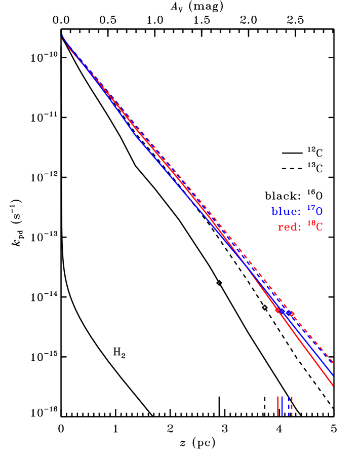
Figure 9: Photodissociation rates of H₂ and the six CO isotopologues as a function of depth into translucent cloud model C2$\alpha$ with $n_{\mathrm{H}}=300$ cm^-3, $T_{\mathrm{gas}}=50$ K and $\chi=1$. Attenuation by dust is included. The diamonds and corresponding markers on the bottom axis indicate the depth at which $\@element[+]{\mathrm{He}}$ takes over from UV radiation as the dominant destroyer for each isotopologue.

The extent to which each isotopologue is fractionated can easily be seen from the cumulative column density ratios when they are normalised to ¹²CO and the isotope ratios:

$$\mathcal{R}_{i}(z)=\frac{N_{z}(^{x}\mathrm{C}^{y}\mathrm{O})}{N_{z}(^{12}\mathrm{CO})}\frac{[\@element[12]{\mathrm{C}}]}{[\@element[x]{\mathrm{C}}]}\frac{[\@element[16]{\mathrm{O}}]}{[\@element[y]{\mathrm{O}}]}\,,$$ (9)

with $[X]$ the elemental abundance of isotope $X$ and

$$N_{z}(^{x}\mathrm{C}^{y}\mathrm{O})(z)=\int_{0}^{z}n(^{x}\mathrm{C}^{y}\mathrm{O})\mathrm{d}z^{\prime}\,$$ (10)

the cumulative column density. A plot of $\mathcal{R}(^{13}\mathrm{CO})$ as function of depth (Fig. 10) shows the same trends as the model data in Fig. 8: the amount of ¹³CO is reduced ($\mathcal{R}<1$) up to a certain depth and is enhanced ($\mathcal{R}>1$) further in by isotope-exchange reactions. We only see $\mathcal{R}<1$ for C¹⁷O and C¹⁸O because $\@element[+][17]{\mathrm{O}}$ and $\@element[+][18]{\mathrm{O}}$ never become abundant enough to convert C¹⁶O in a reaction similar to Reaction (7). Photodissociation ceases to be the dominant destruction mechanism for C¹⁷O and C¹⁸O around $z=4$ pc (Fig. 9), so it can no longer cause substantial fractionation and $\mathcal{R}$ gradually returns to unity.

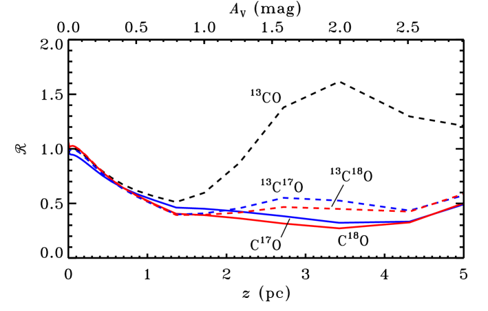
Figure 10: Cumulative column densities of the CO isotopologues normalised to ¹²CO and the elemental isotopic abundances (Eq. (9)) as a function of depth into translucent cloud model C2$\alpha$.

The remaining two isotopologues, ¹³C¹⁷O and ¹³C¹⁸O, experience the $\@element[13]{\mathrm{C}}$ and $\@element[17]{\mathrm{O}}$/$\@element[18]{\mathrm{O}}$ fractionation simultaneously. Isotope exchange enhances their abundances relative to C¹⁷O and C¹⁸O in the same manner and at the same depths as it enhances the abundance of ¹³CO relative to ¹²CO. However, isotope-selective photodissociation is a stronger effect for the two heaviest isotopologues, so $\mathcal{R}$ remains less than unity. This result holds across our entire grid of translucent cloud models.

6.2 Photon-dominated regions

Photon-dominated regions (PDRs) form another type of objects where photodissociation is a key process in controlling the CO abundance. Their densities are higher ($n_{\mathrm{H}}$ up to $\sim$$10^{6}$ cm^-3) than those of diffuse and translucent clouds and they are exposed to stronger UV fields ($\chi$ up to $\sim$$10^{6}$; Hollenbach & Tielens 1997). Observational efforts have mostly gone into mapping the structure of PDRs, so CO column densities are tabulated only for a small number of sources. For most of these the column density of neutral carbon has also been determined. There are no direct measurements of H₂ column densities; instead, $N(\mathrm{H}_{2})$ is usually obtained from $N(^{12}\mathrm{CO})$ using a typical abundance ratio between the two species (e.g., Frerking et al. 1982).

We present here the results from our combined photodissociation and chemistry model for a grid of physical parameters appropriate for PDRs: $T_{\mathrm{gas}}=50$, 80 and 100 K, $n_{\mathrm{H}}=10^{3}$, $10^{4}$, $10^{5}$ and $10^{6}$ cm^-3, and $\chi=10^{3}$, $10^{4}$ and $10^{5}$. The excitation temperatures of CO and H₂ are set equal to $T_{\mathrm{gas}}$. Where necessary, we expand the number of rotational levels of CO beyond the default limit of $J^{\prime\prime}$=7, and likewise for H₂ (see Sect. 4.4). UV pumping increases the population in the $v^{\prime\prime}$=0, $J^{\prime\prime}$¿3 and $v^{\prime\prime}$¿0 levels of H₂. However, this does not affect the CO photodissociation rates at these temperatures, so the level population of H₂ is simply taken as fully thermal. The models are run to an $A_{\mathrm{V}}$ of 30 mag and are otherwise unchanged from the previous section.

Figure 11 shows the relationship between the column densities of ¹²CO and $\@element[12]{\mathrm{C}}$ for a large series of depths steps from our grid. The data for $n_{\mathrm{H}}=10^{4}$ and $10^{6}$ cm^-3 are omitted for reasons of clarity. Overplotted are column densities determined towards a number of positions in different PDRs (Beuther et al. 2000; Kamegai et al. 2003; Kramer et al. 2008; Sun et al. 2008). Figure 5a of Mookerjea et al. (2006) contains additional data for several dozen positions in the PDRs in Cepheus B. In none of these cases was the ¹²CO column density measured directly; instead, it was derived from the ¹³CO or C¹⁸O column density using standard abundance ratios. The spread in both the model predictions and the observational data is large. The column of $\@element[12]{\mathrm{C}}$ for each individual model is nearly constant for $N(^{12}\mathrm{CO})>3\times 10^{17}$ cm^-2, as shown by the solid line connecting the various depth steps for $n_{\mathrm{H}}=10^{5}$ cm^-3, $T_{\mathrm{gas}}=50$ K and $\chi=10^{4}$. The observations seem to correspond more to the lower-density end of the model grid (the plus signs), but the sample is too small and is too scattered to be conclusive.

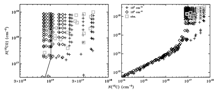
Figure 11: Column density of ¹²CO versus that of $\@element[12]{\mathrm{C}}$ on two different scales. Black: results from our grid of PDR models with $n_{\mathrm{H}}=10^{3}$ cm^-3 (plus signs) and $10^{5}$ cm^-3 (diamonds). The line traces the results for different depth steps at $n_{\mathrm{H}}=10^{5}$ cm^-3, $T_{\mathrm{gas}}=50$ K and $\chi=10^{4}$. Grey squares: observations of Beuther et al. (2000), Kamegai et al. (2003), Kramer et al. (2008) and Sun et al. (2008).

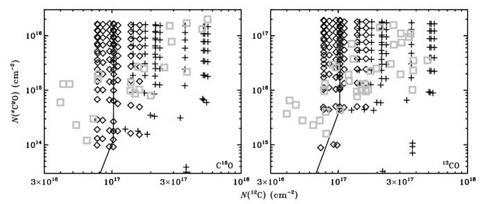
Figure 12: Column densities of C¹⁸O (left) and ¹³CO (right) versus that of $\@element[12]{\mathrm{C}}$. Symbols are as in Fig. 11. See text for references to the observations.

The onset of shielding is seen to occur around $N(^{12}\mathrm{CO})=10^{15}$ cm^-2 in the models. From that point onwards, the low-density models gain more atomic carbon than do the high-density models. For a given column of ¹²CO, the photodissociation rates (or, in other words, the $\@element[12]{\mathrm{C}}$ formation rates) are roughly independent of density, but the destruction of $\@element[12]{\mathrm{C}}$ occurs faster in higher densities. The same argument explained the density dependence of the $N(^{12}\mathrm{CO})/N(\mathrm{H}_{2})$ ratio in the translucent clouds.

The two isotopologues for which column densities have been determined directly are C¹⁸O and ¹³CO (Loren 1989; Gerin et al. 1998; Plume et al. 1999; Beuther et al. 2000; Schneider et al. 2003; Mookerjea et al. 2006; Kramer et al. 2008; Sun et al. 2008). Again, both the observations and the models show a large spread in column densities (Fig. 12). It seems the observations do not trace the high-extinction ($A_{\mathrm{V}}>10$ mag), high-density ($n_{\mathrm{H}}>10^{5}$ cm^-3) material shown in the upper left corner of each panel, but a more detailed study is required to draw any firm conclusions on this point. $N(^{12}\mathrm{CO})$, $N(\mathrm{C}^{18}\mathrm{O})$ and $N(^{13}\mathrm{CO})$ are mutually well correlated in both the observations and the models, but significant deviations can easily occur at specific depths due to the different photodissociation rates. When using standard abundance ratios to derive the column density of ¹²CO from that of another isotopologue, as was done for all cases in Fig. 11, the result will generally be accurate to at best a factor of two.

6.3 Circumstellar disks

6.3.1 Model setup

Low-mass stars like our own Sun are formed through the gravitational collapse of a cold molecular cloud. As the young star grows at the centre, it gathers part of the remaining cloud material into a circumstellar disk. It is inside this disk that planets are formed, so its chemical composition is of great interest. The physical structure of the disk may be simplified as consisting of a cold, dense region near the midplane, covered by a warmer region of lower density. This surface layer intercepts the star’s radiation and shows many similarities to common PDRs.

We adopt the standard disk model of D’Alessio et al. (1999), whose chemistry has been studied extensively (Aikawa et al. 2002; van Zadelhoff et al. 2003; Jonkheid et al. 2004). The star, a T Tauri type, has a mass of 0.5 $M_{\odot}$, a radius of 2 $R_{\odot}$ and an effective temperature of 4000 K. It is surrounded by a disk of mass 0.07 $M_{\odot}$ and outer radius 400 AU. The disk is accreting onto the star at a constant rate of $10^{-8}$ $M_{\odot}$ yr^-1 and its viscosity is characterised by $\alpha=0.01$. We focus on a vertical slice through the disk at a radius of 105 AU, where the surface is located at a height of $z=120$ AU. This slice is irradiated from the top by a radiation field with an effective UV intensity of 516 times that of the interstellar radiation field. Following van Zadelhoff et al., we adopt two spectral shapes: the Draine field and a 4000 K blackbody spectrum. The latter is very weak in the wavelength range where CO is photodissociated. We adopt again the chemical network from Sect. 6.1.1, and we set the gas temperature equal to the dust temperature from the D’Alessio et al. model. Given the high densities ($2\times 10^{4}$ cm^-3 at the surface and more than $10^{9}$ cm^-3 at the midplane), we also use $T_{\mathrm{gas}}$ for $T_{\mathrm{ex}}(\mathrm{CO})$ and $T_{\mathrm{ex}}(\mathrm{H}_{2})$. As in the PDR models, UV pumping of H₂ does not affect the CO photodissociation rates, so the H₂ level populations are taken as fully thermal.

In reality, disks are not irradiated by the Draine field or a pure blackbody. For example, T Tauri stars typically show UV emission in excess of these simple model spectra. Many of them also emit X-rays from accretion hotspots. As shown by van Zadelhoff et al. (2003), the photochemistry of the disk can be sensitive to the details of the radiation field. Moreover, the excess emission can be concentrated in a few specific lines such as H i Lyman-$\alpha$. CO cannot be dissociated by Ly-$\alpha$, but it can be by the H i Ly-$\gamma$ line at 972.54 Å through overlap with the $W0$ band at 972.70 Å (No. 25 from Table LABEL:tb:moldata-ls). A detailed treatment of these effects is beyond the scope of the current work.

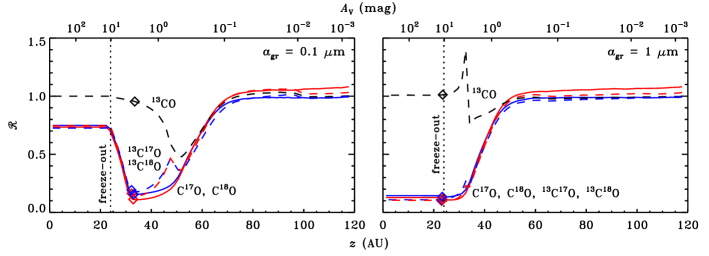
Figure 13: Cumulative column densities of the CO isotopologues normalised to ¹²CO and the elemental isotopic abundances (Eq. (9)) as a function of height at a radius of 105 AU in our disk model with the Draine field and dust grains of 0.1 $\mu$m (left) or 1 $\mu$m (right). CO freezes out below 24 AU. The diamond symbols indicate where H${}_{3}^{+}$ takes over from UV photons as the main destroyer of each isotopologue.

6.3.2 Isotopologue ratios

The depth dependence of the photodissociation rates in the disk, illuminated by the Draine field, is qualitatively the same as in the cloud and PDR models from Sects. 6.1 and 6.2. Several quantitative differences arise because of the different UV intensity and the higher densities. The profiles of the normalised column density ratios, $\mathcal{R}$ (Eq. (9)), do not show any enhancement in ¹³CO. Moving down from the surface, suprathermal chemistry initially prevents the formation of ¹³CO from ¹²CO and $\@element[+][13]{\mathrm{C}}$. The Alfvén waves penetrate to $N(\mathrm{H}_{2})=4\times 10^{20}$ cm^-2, which translates here to a height of about 50 AU. The absence of suprathermal chemistry below that point allows $\mathcal{R}(^{13}\mathrm{CO})$ to increase again. However, the $\@element[+][13]{\mathrm{C}}$ abundance decreases at the same time, and $\mathcal{R}(^{13}\mathrm{CO})$ never gets above unity. This is consistent with the $N(^{12}\mathrm{CO})/N(^{13}\mathrm{CO})$ ratios of more than 69 determined for the disks around HL Tau, AB Aur and VV CrA (Brittain et al. 2005; Schreyer et al. 2008; Smith et al. 2009).

In terms of local abundances, our results show a trend opposite to the model by Woods & Willacy (2009). Moving up vertically from the midplane at a given radius, their $n(^{12}\mathrm{CO})/n(^{13}\mathrm{CO})$ abundance ratio initially remains nearly constant, then drops to a lower value, and finally shows a shallow rise for the remainder of the column. We also find a constant ratio at first, but then we get a rise (equivalent to $\mathcal{R}(^{13}\mathrm{CO})<1$) and a gradual decrease back to the elemental ratio of 69. The difference is due to the absence of suprathermal chemistry in the Woods & Willacy model. Suprathermal chemistry effectively shuts down the isotope-exchange reactions, leaving photodissociation (which increases $n(^{12}\mathrm{CO})/n(^{13}\mathrm{CO})$) as the only fractionation mechanism. Additional observations of ¹²CO and ¹³CO in circumstellar disks are required to ascertain whether isotope exchange or selective photodissociation is the key process in controlling the ratio of the abundances of these two species.

For C¹⁷O and C¹⁸O, $\mathcal{R}$ is $\sim$1 from the disk surface down to 70 AU. It then gradually drops to $\sim$0.1 due to their photodissociation rates being higher than that of ¹²CO. Shielding of C¹⁷O and C¹⁸O sets in around 32 AU, so that photodissociation no longer causes isotope fractionation and $\mathcal{R}$ increases again. However, it does not reach a value of unity. Below 24 AU, the temperature is low enough that most of the CO freezes out onto the dust grains. The tiny amount remaining in the gas phase does not add to the column density, so $\mathcal{R}$ is effectively frozen at 0.75 and 0.73 (Fig. 13). The corresponding column density ratios are $N(^{12}\mathrm{CO})/N(\mathrm{C}^{17}\mathrm{O})=2700$ and $N(^{12}\mathrm{CO})/N(\mathrm{C}^{18}\mathrm{O})=760$. Both values are consistent with the degree of fractionation determined for the disk around the T Tauri star VV CrA (Smith et al. 2009).

6.3.3 Model variations

If we illuminate the disk by a 4000 K blackbody (spectrum C from van Zadelhoff et al. 2003), it does not receive enough photons in the 912–1118 Å range to cause substantial photodissociation of CO. Instead, the non-isotope-selective reactions with $\@element[+]{\mathrm{He}}$ and H${}_{3}^{+}$ are the main destruction mechanisms even at the top of our vertical slice at $R=105$ AU. The normalised column density ratios therefore remain unity at all heights. Adding the interstellar UV field at $\chi=1$ to the 4000 K blackbody spectrum allows CO to be photodissociated again in the surface layers. The isotope fractionation returns, but only partially, because the UV field is still weaker than in the original case. Freeze-out now locks $\mathcal{R}(\mathrm{C}^{17}\mathrm{O})$ and $\mathcal{R}(\mathrm{C}^{18}\mathrm{O})$ at 0.86 and 0.85 instead of $\sim$0.75. Clearly, some UV component is required in the irradiating spectrum to get isotope fractionation through the photodissociation of CO, but it does not have to be a very strong component: the interstellar UV field already has a significant effect in this model.

Another parameter to be varied is the grain size. The disk model so far contained small dust grains, with an average size of 0.1 $\mu$m. Grain growth is an inevitable step towards planet formation and is indeed known to occur in disks (van Boekel et al. 2003; Przygodda et al. 2003; Lommen et al. 2007). Larger grains cause less extinction in the UV (Shen et al. 2004), so CO can be photodissociated deeper into the disk. Grain growth also affects the H₂ formation rate: the rate is inversely proportional to approximately the square of the grain radius (Jonkheid et al. 2006). The right panel of Fig. 13 shows the normalised vertical column density ratios at a radius of 105 AU for an average grain size of 1 $\mu$m. The onset of fractionation occurs at a lower altitude than in the 0.1 $\mu$m case: 55 AU instead of 75 AU. The slower formation rate of H₂ has a direct influence on the formation of CO through the pathway starting with Reaction (4). There is less H₂ and CO in the disk’s surface layers when we increase the grain size, so we have to go down deeper before ¹²CO becomes self-shielding and isotope fractionation sets in. At the same time, the weaker continuum extinction allows the UV radiation to penetrate deeper, so the isotope-selective photodissociation goes on to lower altitudes. The spike in $\mathcal{R}(^{13}\mathrm{CO})$ to 1.4 at 30 AU is due to a narrow zone where the temperature is relatively low (35 K), the Alfvén waves do not reach, and the $\@element[+][13]{\mathrm{C}}$ abundance is high enough to convert ¹²CO into ¹³CO. The model with 0.1 $\mu$m grains also has a narrow zone with a high $\@element[+][13]{\mathrm{C}}$ abundance and no suprathermal chemistry, but the kinetic temperature in this zone is 50 K. There is still some conversion of ¹²CO into ¹³CO at that temperature, but not enough to show as a spike in the normalised column density ratio.

The bigger dust grains also affect the fractionation of C¹⁷O and C¹⁸O. The point at which photodissociation ceases to be the main destruction mechanism now nearly coincides with the point where CO freezes out (Fig. 13). Both species have $\mathcal{R}\approx 0.15$ when this happens, so the ratios are locked at that value. In the small-dust model, the ratios were locked at $\sim$0.75. Observations of face-on disks in principle probe CO all the way to the midplane, so our model predicts that grain growth from 0.1 to 1 $\mu$m can increase the observed fractionation of C¹⁷O and C¹⁸O by a factor of five. The fractionation in the local abundances, which is relevant for incorporating material into comets, increases by the same amount from 0.1 to 1 $\mu$m grains.

All the results so far in this section are for a T Tauri disk. Herbig Ae/Be stars are more massive and more luminous and tend to have warmer disks, where CO may not be frozen out at all. That would prevent $\mathcal{R}$ from being locked as it is in Fig. 13; instead, it would rapidly return to unity for all isotopologues. Observations probing the midplane of such a disk would not find any fractionation in $\@element[17]{\mathrm{O}}$ and $\@element[18]{\mathrm{O}}$ relative to $\@element[16]{\mathrm{O}}$.

6.3.4 Implications for meteorites

Regardless of the grain size and the absence or presence of freeze-out, the model shows $\@element[17]{\mathrm{O}}$ and $\@element[18]{\mathrm{O}}$ to be nearly equally fractionated: $\mathcal{R}$ has very similar values for C¹⁷O and C¹⁸O. The equal photodissociation rates implied by this result are partly due to our choice of molecular parameters. Spectroscopic data on C¹⁷O are still very scarce, so we assume many of its oscillator strengths and predissociation probabilities to have the same value as for C¹⁸O (Sects. 2.3 and 2.4). Still, two important differences remain. First, the elemental abundance of $\@element[18]{\mathrm{O}}$ is higher than that of $\@element[17]{\mathrm{O}}$, resulting in some self-shielding for C¹⁸O (Fig. 1). Second, the shifts of the C¹⁷O lines with respect to ¹²CO are generally somewhat smaller than those of the C¹⁸O lines, so C¹⁷O is more strongly shielded by ¹²CO. Both effects are minor, however, and the photodissociation rates end up being nearly the same.

According to the experiments of Chakraborty et al. (2008), the photodissociation rate due to the $E0$ and $E1$ bands may be up to $\sim$40% higher for C¹⁷O than for C¹⁸O. If we mimic this by artificially increasing the $E0$ and $E1$ oscillator strengths of C¹⁷O by 40%, the overall change in $\mathcal{R}(\mathrm{C}^{17}\mathrm{O})$ is less than 10% at any depth. When the two oscillator strengths are doubled from their standard value, $\mathcal{R}(\mathrm{C}^{17}\mathrm{O})$ changes by at most 20%. In both cases, the change in $\mathcal{R}(\mathrm{C}^{17}\mathrm{O})$ is largest at the top of the disk and gradually decreases for lower altitudes; it is less than 1% below 50 AU.

Observational evidence for equal fractionation of $\@element[17]{\mathrm{O}}$ and $\@element[18]{\mathrm{O}}$ in disks was recently obtained by Smith et al. (2009) for the T Tauri star VV CrA. Their analysis points to isotope-selective photodissociation of CO as the most likely explanation, although they cautioned that more observations are needed to confirm that conclusion. Meanwhile, their observations are consistent with our model results.

A long-standing puzzle in our solar system involves the equal fractionation of $\@element[17]{\mathrm{O}}$ and $\@element[18]{\mathrm{O}}$ in the most refractory phases of meteorites (Clayton et al. 1973). Current evidence points at isotope-selective photodissocation of CO in the solar nebula playing a key role (Clayton 2002; Lyons & Young 2005; Lee et al. 2008). It is generally accepted that the resulting atomic oxygen eventually makes it into the refractory material to produce the observed isotope ratios, but it remains unknown how this actually happens. Any additional mass-independent fractionation during that process must be limited, because photodissociation of CO already reproduces the observed isotope abundance ratios (Young 2007). One important requirement here is to have C¹⁷O and C¹⁸O photodissociate at the same rate, an assumption that had gone untested up to now. Our model confirms they do so in many different environments—including diffuse and translucent clouds, PDRs, and circumstellar disks—even when allowing for the isotope effects suggested by Chakraborty et al. (2008).

Equal (or nearly equal) $\@element[17]{\mathrm{O}}$ and $\@element[18]{\mathrm{O}}$ fractionation also occurs for other oxygen-containing molecules in the model, such as water. The equal fractionation is a clear sign of CO photodissociation playing a key role in the fractionation process. Other fractionation processes, such as isotope-exchange reactions, diffusion, freeze-out and evaporation, depend on the vibrational energies of the isotopologues and are therefore mass-dependent. Specifically, such processes would lead to $\@element[17]{\mathrm{O}}$ being 0.52 times as fractionated as $\@element[18]{\mathrm{O}}$ (Matsuhisa et al. 1978). If mass-independent fractionation processes other than isotope-selective photodissociation play a role in circumstellar disks, they have not been discovered so far (Clayton 2002; Yurimoto & Kuramoto 2004; Lyons & Young 2005). Recently, Kimura et al. (2007) did report on a set of chemical experiments yielding mass-independently fractionated silicates, but they were unable to identify the underlying reaction mechanism. Hence, it remains unknown if this would be relevant for disks. Self-shielding in O₂ (Thiemens & Heidenreich 1983) is unimportant because O₂ never becomes abundant enough to become a significant source of atomic O.

7 Conclusions

This paper presents an updated model, based on the method of van Dishoeck & Black (1988), for the photodissociation of carbon monoxide (CO) and its heavier isotopologues. It contains recent spectroscopic data from the literature and produces a photodissociation rate of $2.6\times 10^{-10}$ s^-1 in the interstellar medium, 30% higher than currently adopted values. Our model is the first to include C¹⁷O and ¹³C¹⁷O and we apply it to a broader range of model parameters than has been done before. The main results are as follows:

• Self-shielding is very important for ¹²CO and somewhat so for C¹⁸O and ¹³CO. The rare isotopologues ¹³C¹⁷O and ¹³C¹⁸O have the highest photodissociation rate at most depths into a cloud or other object. The rates of C¹⁷O and C¹⁸O are very similar at all depths, but details in the line overlap and self-shielding can cause mutual differences of up to 30% (Sects. 3.3 and 6.1.4).

• When coupled to a chemical network, the model reproduces column densities observed towards diffuse clouds and PDRs. It shows that the large spread in observed $N(^{12}\mathrm{CO})/N(^{13}\mathrm{CO})$ ratios may be due to a combination of isotope-selective photodissociation and suprathermal chemistry (Sect. 6.1.3).

• Photodissociation of CO is more strongly isotope-selective in cold gas than in warm gas (Sect. 4).

• The results from the full computation are well approximated by a grid of pre-computed shielding functions, intended for easy use in various other models. Shielding functions are provided for a range of astrophysical parameters (Sect. 5).

• Grain growth in circumstellar disks increases the vertical range in which CO can be photodissociated. If photodissociation is still important at the point where CO freezes out onto the grains, the observable gas-phase column density ratios $N(^{12}\mathrm{CO})/N(\mathrm{C}^{17}\mathrm{O})$ and $N(^{12}\mathrm{CO})/N(\mathrm{C}^{18}\mathrm{O})$ may become an order of magnitude larger than the initial isotopic abundance ratios (Sect. 6.3.3).

• Without a far-UV component in the irradiating spectrum, isotope fractionation through the photodissociation of CO is not possible. The interstellar radiation field can already cause substantial fractionation in disks (Sect. 6.3.3).

• The isotope-selective nature of the CO photodissociation results in mass-independent fractionation of $\@element[17]{\mathrm{O}}$ and $\@element[18]{\mathrm{O}}$. Column density ratios computed for a circumstellar disk agree well with recent observations. Our model supports the hypothesis that the photodissociation of CO is responsible for the anomalous $\@element[17]{\mathrm{O}}$ and $\@element[18]{\mathrm{O}}$ abundances in meteorites (Sect. 6.3.4).

1

Table 14: New molecular data for ¹²CO.^a

Bandb	ER90b	$\lambda_{0}$		$\nu_{0}$		ID		$v^{\prime}$	$f_{\mathrm{v}^{\prime}0}$		$A_{\mathrm{tot}}$	$\eta$		$B_{\mathrm{v}}^{\prime}$		$D_{\mathrm{v}}^{\prime}$		$\omega_{\mathrm{e}}^{\prime}$		$\omega_{\mathrm{e}}x_{\mathrm{e}}^{\prime}$		References	Notes
#	#	(Å)		(cm-1)							(s-1)			(cm-1)		(cm-1)		(cm-1)		(cm-1)
A01A	A07A	912.	7037	109564.	6		${}^{1}\Pi$	0	3.	4(-3)	1(10)	1.	00	1.	9226	5.	9(-5)	2169.	8	13.	29	1	c
B01B	B07B	913.	4002	109481.	0	$(5p\sigma)$	${}^{1}\Sigma^{+}$	1	1.	7(-3)	9(10)	1.	00	1.	829	1.	0(-5)	2214.	2	15.	15	1,2	d
C01C	C07C	913.	4255	109478.	0	$(5p\pi)$	${}^{1}\Pi$	1	1.	7(-3)	1(10)	1.	00	1.	9568	1.	0(-4)	2214.	2	15.	15		d
D01D	D07D	913.	6678	109449.	0		${}^{1}\Sigma^{+}$	2	2.	7(-2)	9(10)	1.	00	1.	7781	5.	4(-5)	2169.	8	13.	29	1,2,3	c
A02A	A08A	915.	7258	109203.	0	$(6p\pi)$	${}^{1}\Pi$	0	2.	0(-3)	1(11)	1.	00	1.	5796	6.	737(-6)	1562.	8	13.	93		e,f
B02B	B08B	915.	9708	109173.	8	$(6p\sigma)$	${}^{1}\Sigma^{+}$	0	7.	9(-3)	1(11)	1.	00	1.	685	1.	0(-4)	2214.	2	15.	15	3	d
03	A09A	917.	2721	109018.	9		${}^{1}\Pi$	2	2.	3(-2)	5(11)	1.	00	1.	671	7.	2(-5)	2169.	8	13.	29	2	c
04	B09B	919.	2097	108789.	1	$(6s\sigma)$	${}^{1}\Sigma^{+}$	0	2.	8(-3)	1(11)	1.	00	2.	1357	4.	633(-5)	2214.	2	15.	15	4,5	d
05	C09C	920.	1410	108679.	0	$I^{\prime}(5s\sigma)$	${}^{1}\Sigma^{+}$	1	2.	8(-3)	1(11)	1.	00	1.	9050	6.	0(-6)	2291.	2	0.	0		g
06	10	922.	7561	108371.	0	$(5d\sigma)$	${}^{1}\Sigma^{+}$	0	6.	3(-3)	3(11)	1.	00	1.	9675	6.	318(-6)	2214.	2	15.	15		d,h
07	11	924.	6309	108151.	3		${}^{1}\Sigma^{+}$	1	5.	2(-3)	1(11)	1.	00	1.	8669	4.	0(-5)	2169.	8	13.	29		c
08	12	925.	8093	108013.	6	$W(3s\sigma)$	${}^{1}\Pi$	3	2.	0(-2)	4(11)	1.	00	1.	6506	1.	1(-4)	1745.	1	$-4$.	22	6	g,i
09	13	928.	6575	107682.	3		${}^{1}\Pi$	2	6.	7(-3)	4(10)	1.	00	1.	936	3.	1(-5)	2169.	8	13.	29	1,2,3	c
10	14	930.	0611	107519.	8		${}^{1}\Pi$	2	6.	3(-3)	1(11)	1.	00	1.	8202	2.	6(-5)	2169.	8	13.	29		c
11	A15A	931.	0744	107402.	8		${}^{1}\Pi$	0	6.	0(-3)	1(11)	1.	00	1.	650	1.	0(-5)	2169.	8	13.	29		c
12	B15B	931.	6547	107335.	9	$(5p\pi)$	${}^{1}\Pi$	0	1.	2(-2)	3(11)	1.	00	1.	8682	4.	3(-5)	2214.	2	15.	15	2	d,j
13	C15C	933.	0583	107174.	4	$(5p\sigma)$	${}^{1}\Sigma^{+}$	0	2.	2(-2)	3(10)	1.	00	2.	128	1.	0(-5)	2214.	2	15.	15	1,2	d,i
14	16	935.	6638	106876.	0		${}^{1}\Sigma^{+}$	2	3.	8(-3)	3(11)	1.	00	1.	95	0.	0	2169.	8	13.	29	5	c
15	17	939.	9574	106387.	8	$I^{\prime}(5s\sigma)$	${}^{1}\Sigma^{+}$	0	2.	1(-2)	1(12)	1.	00	2.	0365	8.	8(-5)	2291.	2	0.	0	4	g,j
16	18	941.	1685	106250.	9	$W(3s\sigma)$	${}^{1}\Pi$	2	3.	1(-2)	1(11)	1.	00	1.	6224	$-1$.	3(-5)	1745.	1	$-4$.	22	1,6	g,i,k
17	19	946.	2860	105676.	3	$(4d\sigma)$	${}^{1}\Sigma^{+}$	0	7.	6(-3)	1(11)	1.	00	1.	8952	1.	73(-5)	2214.	2	15.	15	1,2,3	d
18	20	948.	3860	105442.	3	$L(4p\pi)$	${}^{1}\Pi$	1	2.	8(-3)	1(10)	0.	99	1.	9606	1.	0(-5)	2170.	5	0.	0		g
19	21	950.	0429	105258.	4	$H(4p\sigma)$	${}^{1}\Sigma^{+}$	1	2.	2(-2)	1(12)	1.	00	1.	9436	4.	4(-5)	2203.	7	0.	0	4	g,j
20	22	956.	2369	104576.	6	$W(3s\sigma)$	${}^{1}\Pi$	1	1.	6(-2)	7(11)	1.	00	1.	5696	5.	8(-5)	1745.	1	$-4$.	22	6	g
21	24	964.	3973	103691.	7	$J(4s\sigma)$	${}^{1}\Sigma^{+}$	1	2.	8(-3)	3(11)	1.	00	1.	9202	9.	0(-6)	2235.	7	0.	0		g
22	25	968.	3187	103271.	8	$L(4p\pi)$	${}^{1}\Pi$	0	1.	4(-2)	2(9)0	0.	96	1.	9598	7.	06(-6)	2170.	5	0.	0	7,8,9	g,i,k
23	26	968.	8815	103211.	8	$L^{\prime}(3d\pi)$	${}^{1}\Pi$	1	1.	2(-2)	2(11)	1.	00	1.	754	1.	0(-5)	2214.	2	15.	15	1,2,3,9	d,k
24	27	970.	3588	103054.	7	$K(4p\sigma)$	${}^{1}\Sigma^{+}$	0	3.	4(-2)	2(10)	0.	99	1.	9166	5.	99(-5)	2203.	7	0.	0	1,2,3,9	g
25	28	972.	6996	102806.	7	$W(3s\sigma)$	${}^{1}\Pi$	0	1.	7(-2)	1(10)	0.	97	1.	5664	9.	7(-5)	1745.	1	$-4$.	22	1,3,6	g,i,k
26	29	977.	3996	102312.	3	$W^{\prime}(3s\sigma)$	${}^{3}\Pi$	2	1.	8(-3)	4(11)	1.	00	1.	5417	8.	0(-6)	1562.	8	13.	93	1,2,3	f,k
27	30	982.	5914	101771.	7	$F(3d\sigma)$	${}^{1}\Sigma^{+}$	1	4.	8(-4)	3(11)	1.	00	1.	8506	1.	4(-5)	2030.	0	0.	0		g
28	31	985.	6490	101456.	0	$J(4s\sigma)$	${}^{1}\Sigma^{+}$	0	1.	5(-2)	1(12)	1.	00	1.	9247	5.	1(-5)	2235.	7	0.	0	4	g,j
29	32	989.	7952	101031.	0	$G(3d\pi)$	${}^{1}\Pi$	0	4.	6(-4)	1(11)	1.	00	1.	9632	1.	1(-5)	2214.	2	15.	15		d
30	33	1002.	5897	99741.	7	$F(3d\sigma)$	${}^{1}\Sigma^{+}$	0	7.	9(-3)	3(11)	1.	00	1.	8077	2.	2(-4)	2030.	0	0.	0		g
31	37	1051.	7134	95082.	9	$E(3p\pi)$	${}^{1}\Pi$	1	3.	6(-3)	6(9)0	0.	96	1.	9280	6.	64(-6)	2238.	8	42.	51	10,11,12,13	k
32	38	1063.	0880	94065.	6	$C(3p\sigma)$	${}^{1}\Sigma^{+}$	1	3.	0(-3)	2(9)0	0.	56	1.	9238	6.	25(-6)	2175.	9	14.	76	14,15,16
33	39	1076.	0796	92929.	9	$E(3p\pi)$	${}^{1}\Pi$	0	6.	8(-2)	1(9)0	0.	80	1.	9527	6.	34(-6)	2238.	8	42.	51	13,15,17,18	k

Table 14: continued.

• (1) $\lambda_{0}$ and $\nu_{0}$ from Ubachs et al. (1994); (2) $A_{\mathrm{tot}}$ from Ubachs et al. (1994); (3) $B_{\mathrm{v}}^{\prime}$ and $D_{\mathrm{v}}^{\prime}$ from Ubachs et al. (1994); (4) $\lambda_{0}$ and $\nu_{0}$ from vDB88; (5) $B_{\mathrm{v}}^{\prime}$ and $D_{\mathrm{v}}^{\prime}$ from vDB88; (6) $f_{\mathrm{v}^{\prime}0}$ and $A_{\mathrm{tot}}$ from Eidelsberg et al. (2006); (7) $\lambda_{0}$, $\nu_{0}$, $B_{\mathrm{v}}^{\prime}$ and $D_{\mathrm{v}}^{\prime}$ from Cacciani et al. (2002); (8) $A_{\mathrm{tot}}$ from Drabbels et al. (1993); (9) $f_{\mathrm{v}^{\prime}0}$ from Eidelsberg et al. (2004); (10) $\lambda_{0}$, $\nu_{0}$, $B_{\mathrm{v}}^{\prime}$ and $D_{\mathrm{v}}^{\prime}$ from Ubachs et al. (2000); (11) $f_{\mathrm{v}^{\prime}0}$ from Eidelsberg et al. (2006); (12) $A_{\mathrm{tot}}$ from Ubachs et al. (2000); (13) $\omega_{\mathrm{e}}^{\prime}$, $\omega_{\mathrm{e}}x_{\mathrm{e}}^{\prime}$ from Kepa (1988); (14) $\lambda_{0}$, $\nu_{0}$, $A_{\mathrm{tot}}$, $B_{\mathrm{v}}^{\prime}$ and $D_{\mathrm{v}}^{\prime}$ from Cacciani et al. (2001); (15) $f_{\mathrm{v}^{\prime}0}$ from Federman et al. (2001); (16) $\omega_{\mathrm{e}}^{\prime}$, $\omega_{\mathrm{e}}x_{\mathrm{e}}^{\prime}$ from Tilford & Vanderslice (1968); (17) $\lambda_{0}$, $\nu_{0}$, $B_{\mathrm{v}}^{\prime}$ and $D_{\mathrm{v}}^{\prime}$ from Cacciani & Ubachs (2004); (18) $A_{\mathrm{tot}}$ from Cacciani et al. (1998)

• $\lambda_{0}$, $\nu_{0}$, ID and $v^{\prime}$ from Eidelsberg et al. (1992), $f_{\mathrm{v}^{\prime}0}$, $A_{\mathrm{tot}}$, $B_{\mathrm{v}}^{\prime}$ and $D_{\mathrm{v}}^{\prime}$ from ER90, unless noted otherwise. All $\eta$ are recomputed from the $f_{\mathrm{v}^{\prime}0}$ and $A_{\mathrm{tot}}$. The notation $a(b)$ in this and following tables means $a\times 10^{b}$. Many values are rounded off from higher-precision values in the references.

• The numbering follows vDB88. Their bands 1 and 2 are split into four and two components. The corresponding ER90 indices are also given.

• $\omega_{\mathrm{e}}^{\prime}$ and $\omega_{\mathrm{e}}x_{\mathrm{e}}^{\prime}$ from the CO ground state (Guelachvili et al. 1983). $\omega_{\mathrm{e}}y_{\mathrm{e}}^{\prime}$ and $\omega_{\mathrm{e}}z_{\mathrm{e}}^{\prime}$ (not listed) are included in the model.

• $\omega_{\mathrm{e}}^{\prime}$ and $\omega_{\mathrm{e}}x_{\mathrm{e}}^{\prime}$ from the CO⁺ $X\,^{2}\Sigma^{+}$ state (Haridass et al. 2000).

• $B_{\mathrm{v}}^{\prime}$ and $D_{\mathrm{v}}^{\prime}$ from the CO⁺ $A\,^{2}\Pi$ state (Haridass et al. 2000).

• $\omega_{\mathrm{e}}^{\prime}$ and $\omega_{\mathrm{e}}x_{\mathrm{e}}^{\prime}$ from the CO⁺ $A\,^{2}\Pi$ state (Haridass et al. 2000). $\omega_{\mathrm{e}}y_{\mathrm{e}}^{\prime}$ (not listed) is included in the model.

• Vibrational constants derived from the different $\nu_{0}$ in one of six vibrational series: bands 30–27, 28–21, 25–20–16–8, 24–19, 22–18 or 15–5.

• $B_{\mathrm{v}}^{\prime}$ and $D_{\mathrm{v}}^{\prime}$ from the CO⁺ $X\,^{2}\Sigma^{+}$ state (Haridass et al. 2000).

• $A_{\mathrm{tot}}$ depends on parity and/or rotational level (see Table 3). $A_{\mathrm{tot}}$ and $\eta$ are listed here for $J^{\prime}$=0 and $f$ parity.

• $B_{\mathrm{v}}^{\prime}$ and $D_{\mathrm{v}}^{\prime}$ computed from the C¹⁸O values of ER90.

• $B_{\mathrm{v}}^{\prime}$ and $D_{\mathrm{v}}^{\prime}$ depend on parity (see Table 2); values are listed here for $f$ parity.