Abstract

We consider a model of static cosmic string loops in type IIB string theory, where the strings wrap cycles within the internal space. The strings are not topologically stabilised, however the presence of a lifting potential traps the windings giving rise to kinky cycloops. We find that PBH formation occurs at early times in a small window, whilst at late times we observe the formation of dark matter relics in the scaling regime. This is in stark contrast to previous predictions based on field theoretic models. We also consider the PBH contribution to the mass density of the universe, and use the experimental data to impose bounds on the string theory parameters.

1 Introduction

In recent years there has been a renewed effort to test string theory in a cosmological context. This is due in part to the availability of increasingly precise data from experiments such as WMAP [1] and SDSS [2]. However, it is also due to theoretical advances which have resulted in a better understanding of the compactifications of the theory down to $(3+1)$-dimensions. Since such compactifications are typically warped this means that mass scales in the effective theory can be significantly reduced. One important consequence of this is that superstrings may have a much smaller tension than first realised [3, 4].

Originally Witten [5] ruled out the notion that $F$-strings could play the role of cosmic-strings because of their extremely high mass density. The un-warped string tension is so large that the presence of cosmic $F$-strings (formed after inflation) would be immediately evident in the CMB. This effectively killed the field until GKP (Giddings-Kachru-Polchinski) [6] showed, in the context of type IIB strings, that by turning on non-trivial fluxes threading cycles in a class of compact manifolds one could obtain highly warped four-dimensional backgrounds. The warping acts in such a way as to reduce the overall tension of any object, and therefore it was possible to evade the observational bounds.

Simultaneously there has also been renewed interest in models of open string inflation. In such models the energy density of the inflaton field(s) is provided by the geometric distance between the $D3$-brane of our universe and parallel branes or anti-branes. Since such branes/anti-branes are charged under massless $RR$-form fields it is expected that large numbers of $F$ and $D$-strings, as well as bound states of multiple strings, will be produced at the end of inflation [4, 7, 8]. Generically these objects are called $(p,q)$-strings, since they are typically a bound state consisting of $p$ $F$-strings and q $D$-strings [9, 10, 11]. Observationally however this raises a potential problem as these strings are not red-shifted away and therefore (presumably) fine tuning is required to restrict their number to $\mathcal{O}(1)$ per Hubble radius at the present epoch. In this paper we will simply assume that some phase of open string inflation has occurred, though it remains an open problem to generate such a configuration in an explicit model of string theory inflation.

Given that these strings exist in a higher dimensional theory, one could also imagine that they wrap cycles within the internal space [12]. Such cycles could be either ”smooth” or ”lumpy” from a four dimensional perspective. A string that wraps a series of internal cycles at separate points in four-dimensional space would appear as a necklace. That is, as a system of monopoles or ”beads” connected by string segments. Alternatively, strings which wrap the compact directions smoothly along their four dimensional length would appear to have a continuously varying mass density. The exact nature of the variation depends on the geometry of the compact space, though in general we would expect the effective tension to be periodic.

Matsuda has proposed that a necklace structure may form from a smoothly varying configuration as the string relaxes to a quasi-stable state [13]. In this case the periodic variation of effective string tension is viewed as the sum of the standard string tension plus a lifting potential in the (angular) compact directions. If the angular directions are flat the energy of the string is minimised for a smoothly varying configuration, resulting in a constant effective string tension, but in the presence of a potential a necklace structure is energetically favoured. Furthermore the existence, or absence, of a potential affects the stability of the extra-dimensional windings when strings chop off from the network to form loops. In the absence of a lifting potential windings must be stabilised topologically giving rise to objects called ”cycloops”. This is not true for necklace solutions which may exist, at least over cosmologically relevant time scales, even if the compact space is simply connected. The quasi-stability of the necklace solution is discussed in greater detail in section 5.5.

The cosmological consequences of cycloops were first investigated by Avgoustidis and Shellard [14]. They showed that, unlike an ordinary string loop, a decaying cycloop leaves a topologically trapped remnant when it reaches zero radius. This remnant appears as a monopole to a four dimensional observer and may be interpreted as a dark matter particle. Like ordinary string loops, cycloops also have a small probability ($f\sim 10^{-20}$) of collapsing to form PBH’s in the course of their first oscillation. These PBH’s may then decay to leave topologically stable Planck-mass relics, though this possibility has not been thoroughly investigated [14, 13].

By contrast Matsuda has claimed that a large fraction $f\sim 1$ of all necklace loops eventually collapse to form PBH’s via a separate necklace-specific process. This claim is based on the assumption that mass-energy may only be lost, via gravitational wave emission, from the four-dimensional string segments, leaving the bead mass unchanged. Thus when the necklace loop reaches its minimum radius it will undergo collapse if the mass of the beads is large enough to produce a Schwarzschild radius greater than the string width. He therefore proposed that small loops produced at very early times may form stable relics which also act as dark matter candidates. Conversely he argued that loops created at later times would be larger and hence likely to contain enough mass in their beads to cause them to collapse into PBH’s [15].

However this original schematic analysis involved a number of simplifying assumptions, such as the existence of a time-independent lifting potential and hence a constant bead mass for necklace loops formed at different epochs. The initial inter-bead spacing was also assumed to scale like the entropy distance at the time of network formation and the dynamical evolution of the inter-bead distance was modeled by the standard string-monopole network evolution equations, originally proposed by [17].

In the following analysis we attempt to construct a more concrete model of necklace formation based on ideas from type IIB string theory. We calculate the explicit form of the lifting potential for a loop of string with extra-dimensional windings in the Klebanov-Strassler geometry [18, 19]. Using realistic models of winding and loop formation we see that potential itself evolves dynamically resulting in a time dependent bead mass. This shows that the first of these assumptions must be modified, at least for certain backgrounds.

Additionally the decay signature of necklace loops in our model is in many ways the opposite of what Matsuda predicted. We find that PBH formation is favoured at early times with potential dark matter relics forming later. This is indeed an unexpected result [20], though one which appears to follow naturally from the consideration of monopole/bead formation as a dynamical process rather than as the result of a separate phase transition prior to string formation. We argue that this is the correct approach to take when considering monopoles which form from extra-dimensional windings and a comparison of our results with field-theoretic string-monopole networks is given in section 5.6.

In addition to a renewed interest in the role of $F$/$D$-string networks in cosmology there are still many in the physics community devoted to the study of field theoretic cosmic strings [21, 22, 23]. Whilst a stringy origin of the CMB perturbations has been ruled out by observation, the best $\Lambda$ CDM model fit to the data suggests that these strings may contribute at the level of $\sim 10\%$, [24] (for a review see also [25] ) making them extremely important objects to study. Unfortunately a best fit for $(p,q)$ strings, necklaces or cycloops has not yet been investigated, at least at the field theory level [26].

However recent discoveries of dualities between gauge field strings and $F/D$-strings have raised the possibility of unifying these two approaches. Indeed, if string theory really is a theory of everything (TOE), and if we accept Quantum Field Theory (QFT) to be a valid low-energy approximation, we may also hope to find string theory analogues of all field theory phenomena. If therefore we expect topological defects, including strings, to arise generically in symmetry breaking processes, we must investigate the relationship between fundamental strings and field theory strings in much more detail.

The aim of this paper is to consider a simple model of string necklaces in a well understood supergravity background using type IIB string theory, thereby extending the initial phenomenological approach begun in [20]. Following the considerations above therefore we also consider the possible relation of these objects to field theoretic strings, restricting ourselves to generic considerations. Since the background yields an explicit form for the uplifting potential in terms of the number of extra-dimensional windings we may compute the bead mass precisely if this number is known for a string loop formed at any epoch. Following [14] we assume that the motion of a string in the compact space, prior to the chopping off of a loop, is random. This therefore allows us to estimate both the time-dependent bead mass and the average inter-bead distance. We find that the results depend the definition of the parameter $\omega_{l}$, which gives the fraction of the total string length contained in the extra-dimensional windings. Two definitions are suggested: Identifying the inter-bead distance in the string picture with the correlation length in the field theory picture, we see that the first definition leads naturally to a scaling solution - similar to that for field theoretic strings but with a correlation length $L(t)\sim\gamma t$ much smaller than the horizon. The second leads to sub-scaling solution $L(t)\sim t^{\frac{3}{4}}$.

More importantly we are able to compute the PBH mass spectrum produced by collapsing necklaces. Since the mass of an individual necklace depends upon the structure of the internal manifold as well as the string tension, the resulting PBH spectrum yields information about the size of the of the extra dimensions and the warp factor. This in turn influences the background cosmic ray flux via the Hawking radiation of PBH’s expiring at the present epoch. We are thus able to provide observational bounds on string theory parameters using measurements of the extra-galactic gamma-ray flux at 100MeV from the EGRET experiment [27].

An interesting result is that both definitions of $\omega_{l}$ give the same qualitative behaviour with PBH formation occurring only over a limited time period in the early universe. However it must also be noted that the upper and lower limits of this window and hence the resulting bounds on the model parameters do vary significantly in each case.

The layout of the paper is then as follows: In Section 2 we introduce the Klebanov-Strassler geometry which is the supergravity background for the string embedding. In Section 3 we construct the world-volume action for string loops before analysing their stability in Section 4. Section 5 deals with the formation of these loops and their cosmological impact, focusing on the predictions for PBH abundance and Section 6 contains a brief discussion of our main results and suggestions for future work.

We conclude this introduction with a note regarding terminology. The ”necklaces” which are the subject of the present paper and of Matsuda’s original work should not be confused with ”necklaces” formed via other string-monopole interactions. For example, Leblond and Wyman [28] have shown that $D0$-branes (monopoles) may be formed at junctions between strings in a $(p,q)$-string network. The resulting ”necklaces” are of no relation to the ones considered here. Related work can be found in [29, 30, 31, 32].

2 Klebanov-Strassler geometry

The background we wish to consider is that of the Klebanov-Strassler (KS) throat [18, 19] since it is one of the better understood backgrounds of the type IIB theory. Recall that conical singularities are the most generic kind of singularities arising within compactifications of IIB string theory on manifolds of $SU(3)\times SU(3)$ structure [33]. Since explicitly realistic compactifications are difficult to construct, we will take a more phenomenological approach by considering (non-compact) conical backgrounds such as the conifold $T^{1,1}$, that can be glued to a (conformal) Calabi-Yau manifold. Provided we work in a region far from this gluing, we can (locally) work with the conifold geometry without worrying too much about the precise details of the compactification mechanism. With this in mind we can regularise the singular conifold by allowing the $S^{2}$ to shrink to zero size. This is just the deformation of the conifold, which is topologically equivalent to the cotangent bundle over the three-sphere $T^{*}S^{3}$ where the $S^{3}$ has some minimal size.

The solution of Klebanov-Strassler requires the introduction of both $D3$-branes and fractional $D3$-branes in this background [18], where the fluxes back-react on the geometry to create a warped throat. The $RR$-three form flux is threaded through the finite size three-sphere, whilst the $NS$-$NS$ flux wraps the dual (B) cycle as follows,

$$\frac{1}{4\pi^{2}\alpha^{\prime}}\int_{S^{3}}F^{(3)}=M,\hskip 28.45274pt\frac{1}{4\pi^{2}\alpha^{\prime}}\int_{B}H^{(3)}=-K.$$ (2.1)

The fluxes generate a non-trivial warp factor for the full ten-dimensional solution which effectively measures the size of the blow-up contribution along the $S^{2}$ via

$$h(\tau) = 2^{2/3}(g_{s}M\alpha^{\prime})^{2}\epsilon^{-8/3}I(\tau)$$

$$I(\tau) = \int_{\tau}^{\infty}\frac{x\coth(x)-1}{\sinh^{2}(x)}\left(\sinh(2x)-2x\right)dx.$$ (2.2)

For the solution we are considering, we must send $\tau\to 0$, since $\tau$ controls the radius of the $S^{2}$, and therefore the warping approaches a constant value $a_{0}=\rm{Lim}_{\tau\to 0}h(\tau)$, and the ten-dimensional metric is well approximated by the following;

$$ds^{2}=a_{0}^{2}\eta_{\mu\nu}dx^{\mu}dx^{\nu}+R^{2}(d\psi^{2}+\sin^{2}\psi(d\theta^{2}+\sin^{2}\theta d\phi^{2}))$$ (2.3)

with $B^{(2)}\sim C^{(0)}\sim 0$ at the tip, and

$$C^{(2)}=\frac{1}{g_{s}}M\alpha^{\prime}F(\psi)\omega_{2}$$ (2.4)

where $\omega_{2}$ is the volume form along the two-cycle parameterised by $\theta,\phi$, and $F(\psi)\sim\psi-\sin\psi\cos\psi$. In this definition we are explicitly assuming the background gauge choice [8]

$$\theta = \theta_{1}=-\theta_{2}$$

$$\phi = \phi_{1}=-\phi_{2}$$ (2.5)

and $\psi$ is now the azimuthal angle on the $S^{3}$ with $\psi\in(0,2\pi]$ as its fundamental domain. Note also that the $x^{\mu}$ are dimensionful coordinates whilst we define the radius of the three-sphere via,

$$R^{2}=bMg_{s}\alpha^{\prime}$$ (2.6)

where $b$ is a numerical factor and $g_{s}$ is the string coupling, keeping the angular variables dimensionless. It is important to note that the dilaton, and therefore the string coupling, is constant in this background.

In what follows we will assume that (2.3) is representative of a large class of warped geometries, without necessarily having explicit realisation in a fully UV complete construction. In particular this means that we should treat the warping parameter $a_{0}$ as a constant satisfying $0<a_{0}<1$. For the (non-compact) KS solution we find that $a_{0}$ is related to the deformation parameter of the conifold $\epsilon$ via the expression

$$a_{0}^{2}\sim\frac{\tilde{\epsilon}^{4/3}}{R^{2}}$$ (2.7)

where $\tilde{\epsilon}$ is re-scaled to have the correct dimensions and is related to the deformation parameter $\epsilon$ of the warped conifold. The basic point is that the warping varies like $1/g_{s}M$ where we are assuming the supergravity (SUGRA) limit $g_{s}M>>1$ so that, for fixed $R$, constraints on the warping can be interpreted as directly constraining the background geometry. We should also point out that there is nothing special about the deformed conifold solution. One could equally well use the resolved conifold where the $S^{2}$ is blown up instead [34, 35]. Indeed the resulting cosmic-string tension scales directly with the resolution parameter and is therefore highly constrained by observations. The resulting solution is then very similar to the model considered in [37].

Our choice for the background is also inspired in part by the AdS/CFT duality, since the KS geometry is known to be dual to an $\mathcal{N}=1$ confining gauge theory. When viewed from this perspective, the strings are effectively the confining strings of the gauge theory with non-trivial wrapping. Whilst this is interesting in its own right, our motivation will be to model cosmic-necklaces rather than gauge theory necklaces.

3 String loops with non-trivial windings in internal space

The action for both fundamental strings ($F$-strings) and $D1$-branes ($D$-strings) - or in more general $(p,q)$ notation $(1,0)$ and $(0,1)$ strings respectively - in the warped deformed conifold is simply the Nambu-Goto action with additional world-sheet flux, plus a possible Chern-Simons term (for the $D$-string),

$$S=-T_{1}\int d\sigma dt\sqrt{-X}+S_{CS}$$ (3.1)

where $T_{1}$ is the string tension and $X=\rm{det}{X_{ab}}$,

$$X_{ab}=\gamma_{ab}+\lambda F_{ab}$$ (3.2)

where $a,b\in\left\{0,\sigma\right\}$, $\gamma_{ab}$ is the usual induced metric on the world-sheet,

$$\gamma_{ab}=G_{MN}(X(\sigma,t))\partial_{a}X^{M}(\sigma,t)\partial_{b}X^{N}(\sigma,t)$$ (3.3)

and $\lambda=2\pi l_{s}^{2}$. The simple form of the Lagrangian density $\sqrt{-X}$ arises because we are neglecting the coupling of the world-sheet to the $NS$-$NS$ two-form field, which is vanishing in our background (at least in the limit we are considering). The flux tensor is anti-symmetric such that $\lambda F_{00}=\lambda F_{\sigma\sigma}=0$ and $\lambda F_{0\sigma}=-\lambda F_{\sigma 0}$, $\lambda F_{0\sigma}\geq 0$. Note that we are absorbing the definition of the string coupling into the field strength tensor, since this allows us to identify the String frame with the Einstein frame. The Chern-Simons coupling is given by the integral of the pull-back of the $RR$ two-form over the world-sheet, for the case of D-strings,

$$S_{CS}=T_{1}\int d\sigma dtM\alpha^{\prime}(\psi-\sin\psi\cos\psi)d\theta\wedge d\phi$$ (3.4)

However, for the sake of simplicity we choose to ignore this correction in the following analysis and instead concentrate solely on the Nambu-Goto component of the action.

We wish to take the following general ansatz for the string embedding,

$$X^{M}=(t,r(t)\sin\sigma,r(t)\cos\sigma,z_{0},\tau\rightarrow 0,0,0,\psi(\sigma,t),\theta(\sigma,t),\phi(\sigma,t))$$ (3.5)

where $0<\psi\leq 2\pi$, $0<\theta\leq\pi$ and $0<\phi\leq\pi$. This describes a circular string in the Minkowski directions which is wrapped smoothly over the $S^{3}$ in the internal space. Note that in this model the strings sit at the tip of the warped throat. We also make this choice for the sake of simplicity. However there is no a priori reason why we should make this assumption. The more general case would follow the lines of [36]. Using the metric (2.3) and the embedding ansatz (3.5) the action then becomes

$$S=-T_{1}a_{0}^{2}\int d\sigma dt\sqrt{(1-\dot{r}^{2})(r^{2}+a_{0}^{-2}R^{2}s^{\prime 2})-a_{0}^{-2}r^{2}R^{2}\dot{s}^{2}-a_{0}^{-4}\lambda^{2}F^{2}_{0\sigma}-a_{0}^{-4}R^{4}\dot{s}^{2}s^{\prime 2}+a_{0}^{-4}R^{4}(\dot{s}s^{\prime})^{2}}$$ (3.6)

where we have introduced the slightly abusive notation,

$$\dot{s}^{2} = \dot{\psi}^{2}+\sin^{2}\psi(\dot{\theta}^{2}+\sin^{2}\theta\dot{\phi}^{2})$$

$$s^{\prime 2} = \psi^{\prime 2}+\sin^{2}\psi(\theta^{\prime 2}+\sin^{2}\theta\phi^{\prime 2})$$ (3.7)

$$(\dot{s}s^{\prime}) = \dot{\psi}\psi^{\prime}+\sin^{2}\psi(\dot{\theta}\theta^{\prime}+\sin^{2}\theta\dot{\phi}\phi^{\prime})$$

where a dot or dash indicates differentiation with respect to $t$ or $\sigma$ respectively and we have chosen the gauge so as to identify the world-sheet time coordinate with the proper time in the Lorentz frame of the string loop, $t$. We have also included a non-zero ’electric’ gauge field contribution for generality. For the $D$-string case this corresponds to the dissolving of $F$-string charge on the world-sheet and the strings are essentially superconducting.

There are two constants of motion for this configuration, the total energy of the string $H$ and the angular momentum $l$, due to the motion of the string in the internal dimensions^,. We parameterise these conserved charges as follows [37]

$$H=\frac{\partial L}{\partial\dot{q}^{I}}\dot{q}^{I}-L,\hskip 17.07182ptl=\frac{\partial L}{\partial\dot{q}^{I}}q^{\prime I}$$ (3.8)

where $L$ is the Lagrangian and $q^{I}$ are the canonical coordinates which are themselves functions of the world-volume coordinates through $q^{I}=(r(t),\sigma,\psi(\sigma,t),\theta(\sigma,t),\phi(\sigma,t))$. Using (3.6) and neglecting the Chern-Simons term, we find the following expressions for these conserved charges

$$H = T_{1}\int d\sigma\frac{a_{0}^{2}(r^{2}+a_{0}^{-2}R^{2}s^{\prime 2})}{\sqrt{(1-\dot{r}^{2})(r^{2}+a_{0}^{-2}R^{2}s^{\prime 2})-a_{0}^{-2}r^{2}R^{2}\dot{s}^{2}-a_{0}^{-4}\lambda^{2}F^{2}_{0\sigma}-a_{0}^{-4}R^{4}\dot{s}^{2}s^{\prime 2}+a_{0}^{-4}R^{4}(\dot{s}s^{\prime})^{2}}}$$

$$l = T_{1}\int d\sigma\frac{R^{2}r^{2}(\dot{s}s^{\prime})}{\sqrt{(1-\dot{r}^{2})(r^{2}+a_{0}^{-2}R^{2}s^{\prime 2})-a_{0}^{-2}r^{2}R^{2}\dot{s}^{2}-a_{0}^{-4}\lambda^{2}F^{2}_{0\sigma}-a_{0}^{-4}R^{4}\dot{s}^{2}s^{\prime 2}+a_{0}^{-4}R^{4}(\dot{s}s^{\prime})^{2}}}$$

However it is more useful to re-write the Hamiltonian in canonical form using the momenta;

$$P^{2} = \left(\frac{\partial L}{\partial\dot{r}}\right)^{2},\hskip 14.22636pt\Pi^{2}=\left(\frac{\partial L}{\partial\dot{A}}\right)^{2}$$

$$L_{\psi}^{2} = \left(\frac{\partial L}{\partial\dot{\psi}}\right)^{2},\hskip 14.22636ptL_{\theta}^{2}=\left(\frac{\partial L}{\partial\dot{\theta}}\right)^{2},\hskip 14.22636ptL_{\phi}^{2}=\left(\frac{\partial L}{\partial\dot{\phi}}\right)^{2}$$ (3.9)

This will simplify the form of our solutions for stable string windings with non-zero world-sheet flux $\lambda F_{0\sigma}\neq 0$. This is especially true in the static $(l=0)$ case which we will consider in Section 4.

After a long but straight forward calculation we find that the canonical form of the Hamiltonian reduces to,

$$H=\int d\sigma\sqrt{r^{2}+a_{0}^{-2}R^{2}s^{\prime 2}}\sqrt{T_{1}^{2}a_{0}^{4}+\frac{P^{2}}{(r^{2}+a_{0}^{-2}R^{2}s^{\prime 2})}+\frac{\Pi^{2}}{a_{0}^{-4}\lambda^{2}}+\tilde{L_{\psi}^{2}}+\tilde{L_{\theta}^{2}}+\tilde{L_{\phi}^{2}}}$$ (3.10)

where we have written

$$\tilde{L_{\psi}}^{2} = \frac{a_{0}^{4}\dot{\psi}L_{\psi}^{2}}{T_{1}^{2}a_{0}^{2}R^{2}{r^{2}\dot{\psi}+\sin^{2}\psi[\theta^{\prime}(\dot{\psi}\theta^{\prime}-\dot{\theta}\psi^{\prime})+\sin^{2}\theta\phi^{\prime}(\dot{\psi}\phi^{\prime}-\dot{\phi}\psi^{\prime})]}}$$

$$\tilde{L_{\theta}}^{2} = \frac{a_{0}^{4}\dot{\theta}L_{\theta}^{2}}{T_{1}^{2}a_{0}^{2}R^{2}\sin^{2}\psi{r^{2}\dot{\theta}+[\psi^{\prime}(\dot{\theta}\psi^{\prime}-\dot{\psi}\theta^{\prime})+\sin^{2}\psi\sin^{2}\theta\phi^{\prime}(\dot{\theta}\phi^{\prime}-\dot{\phi}\theta^{\prime})]}}$$ (3.11)

$$\tilde{L_{\phi}}^{2} = \frac{a_{0}^{4}\dot{\phi}L_{\phi}^{2}}{T_{1}^{2}a_{0}^{2}R^{2}\sin^{2}\psi\sin^{2}\theta{r^{2}\dot{\phi}+[\psi^{\prime}(\dot{\phi}\psi^{\prime}-\dot{\psi}\phi^{\prime})+\sin^{2}\psi(\dot{\phi}\theta^{\prime}-\dot{\theta}\phi^{\prime})]}}$$

In the next section we will specify the ansatz (3.5) completely by identifying the functions $\psi(\sigma,t)$, $\theta(\sigma,t)$ and $\phi(\sigma,t)$. We will then use equation (3.10) to determine the stability conditions in the static case by minimising the total energy of the string. Finally we see how this leads naturally to a concrete model of necklace loops in the warped throat scenario when these solutions are perturbed.

4 Stability analysis for string loops in the static $(l=0)$ case and necklace formation

In the static case we assume that there is no motion in the compact dimensions and that the loop is neither expanding nor contracting in Minkowski space. Setting $\dot{\psi}=\dot{\theta}=\dot{\phi}=0$ and $\dot{r}=0$ (or equivalently $L_{\psi}^{2}=L_{\theta}^{2}=L_{\phi}^{2}=0$ and $P^{2}=0$) gives the static potential $V$ (below) and $l=0$ as expected.

$$V=\int d\sigma a_{0}^{2}\sqrt{T_{1}^{2}+\frac{\Pi^{2}}{\lambda^{2}}}\sqrt{r^{2}+a_{0}^{-2}R^{2}s^{\prime 2}}$$ (4.1)

Note that even static strings of this kind may lose mass-energy over time due to the emission of gravitational radiation, causing them to shrink. However we refer here to the stability of extra dimensional-windings in the static gauge over an epoch in which the loop size $r$ and energy $V$ are roughly constant. The shrinking of necklace loops over cosmological time scales and its implications are dealt with explicitly in Section 5.

We must now complete the ansatz (3.5). Choosing $\psi(\sigma,t)$, $\theta(\sigma,t)$, and $\phi(\sigma,t)$ to be such that the angular winding is linear in $\sigma$ , we see

$$\psi(\sigma,t) = 2n_{\psi}\sigma+\psi(t),$$

$$\theta(\sigma,t) = n_{\theta}\sigma+\theta(t),$$ (4.2)

$$\phi(\sigma,t) = n_{\phi}\sigma+\phi(t)$$

where $n_{\psi}$, $n_{\theta}$, $n_{\phi}\in N$ and $0<\sigma\leq 2\pi$ then gives

$$V=\int d\sigma a_{0}^{2}T_{1}\sqrt{1+\frac{\Pi^{2}}{T_{1}^{2}\lambda^{2}}}\sqrt{r^{2}+a_{0}^{-2}R^{2}(4n_{\psi}^{2}+\sin^{2}\psi(n_{\theta}^{2}+\sin^{2}\theta n_{\phi}^{2}))}$$ (4.3)

where $\psi$ and $\theta$ are themselves functions of $\sigma$ and $t$ according to (4).

We see immediately that $V=V(\psi,\theta)$ indicating that the $\phi$-direction is flat, whereas the $\psi$ and $\theta$ directions are ”lifted” by the presence of a potential energy density $\mathcal{V}$ which is the integrand in (4.3).

It is now possible to make a connection between wound strings at the tip of the conifold throat, and the cosmic necklaces predicted generically by Matsuda [13]. First we must determine the conditions under which the wrappings described above are stable, which is done by minimising the total energy $V$. Perturbations of this configuration are then seen to give rise to beads, whose mass can be estimated from the functional form of the potential.

However rather than simply minimising the potential, it is useful (and easier) at this point to develop a physical intuition for the string configuration. Treating $\psi$ and $\theta$ as independent variables, we may sketch the lifting potential (strictly speaking the lifting potential energy density, but from here on these two terms will be used interchangeably) which the string ”sees” throughout the whole $S^{3}$. This is done by plotting the integrand $\mathcal{V}$ in (4.3). The result for the principle range ($0<\psi\leq 2\pi$, $0<\theta\leq\pi$) is shown in Figure 1 for the purposes of illustration.

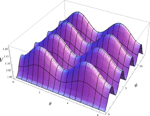
Figure 1: Plot of the static potential $\mathcal{V}$ setting the tension pre-factor term to unity and also $r^{2}=1$ and $a_{0}^{-2}R^{2}=1$.

The critical points and associated field masses may be found by diagonalising the corresponding Hessian matrix. We verify that $\mathcal{V}$ has equal local maxima at positions $(\psi=\frac{(2n+1)\pi}{2},\theta=\frac{(2m+1)\pi}{2})$, saddle points of equal magnitude at $(\psi=\frac{(2n+1)\pi}{2},\theta=m\pi)$ and flat directions which are also local minima (i.e. ”troughs” not ”ridges” or points of inflection) given by $(\psi=n\pi,\theta)$, where $m,n\in Z$. This gives rise to two local maxima, two saddle points and two flat directions in the principle range. The associated field masses are given below.

• $\psi=\frac{(2n+1)\pi}{2}$, $\theta=\frac{(2m+1)\pi}{2}$ (local maxima)

  $$m_{\theta}^{2}=-\frac{T_{1}R^{2}n_{\phi}^{2}}{\sqrt{r^{2}+a_{0}^{-2}R^{2}(4n_{\psi}^{2}+n_{\theta}^{2}+n_{\phi}^{2})}},m_{\psi}^{2}=-\frac{T_{1}R^{2}(n_{\theta}^{2}+n_{\phi}^{2})}{\sqrt{r^{2}+a_{0}^{-2}R^{2}(4n_{\psi}^{2}+n_{\theta}^{2}+n_{\phi}^{2})}}$$ (4.4)

• $\psi=\frac{(2n+1)\pi}{2}$, $\theta=m\pi$ (saddle points)

  $$m_{\theta}^{2}=\frac{T_{1}R^{2}n_{\phi}^{2}}{\sqrt{r^{2}+a_{0}^{-2}R^{2}(4n_{\psi}^{2}+n_{\theta}^{2})}},m_{\psi}^{2}=-\frac{T_{1}R^{2}n_{\theta}^{2}}{\sqrt{r^{2}+a_{0}^{-2}R^{2}(4n_{\psi}^{2}+n_{\theta}^{2})}}$$ (4.5)

• $\psi=n\pi$, $\theta$ (flat directions)

  $$m_{\theta}^{2}=0,m_{\psi}^{2}=\frac{T_{1}R^{2}(n_{\theta}^{2}+sin^{2}\theta n_{\phi}^{2})}{\sqrt{r^{2}+4a_{0}^{-2}R^{2}n_{\psi}^{2}}}$$ (4.6)

It is now intuitively clear that minimal energy configurations correspond to strings wrapping flat directions in the two-dimensional sub-manifold described by $\psi$ and $\theta$. Physically this corresponds to strings wrapping some point in the $S^{3}$ which is uniquely determined by the condition $\psi=n\pi$ for some $n\in Z$. This may be seen from the metric (2.3) and is the reason why $n_{\theta}$ and $n_{\phi}$ do not contribute to the total energy. Even though, technically, $n_{\theta}$,$n_{\phi}\geq 0$ windings around points have zero length and are not physically meaningful. This result is precisely what we should expect, since the minimum energy configuration ought to correspond to a situation in which the string has effectively zero length involved in extra-dimensional windings.

Indeed, we may verify this by substituting $\psi=n\pi$ and setting $\Pi^{2}=0$ in (4.3) that the total energy of a string wrapping flat directions in the potential $\mathcal{V}$ is given by

$$V=2\pi a_{0}^{2}rT_{1}$$ (4.7)

which is simply the rest mass of a string loop with radius $r$ in warped Minkowski space.

This is certainly a very complicated way of verifying an intuitively obvious result but the above analysis will prove useful when we consider perturbations which result in different sections of a single string lying along equivalent local minima. That is, when the string interpolates between degenerate minima (flat directions) in the $(\psi,\theta)$ sub-manifold resulting in the formation of beads.

Note that the flat directions in Figure 1 effectively define degenerate vacuum states for the string. For this reason we propose identifying the inter-bead distance in the string picture with the correlation length of field-theoretic strings. This forms the basis for identifying the field-theoretic parameter $\gamma$ (which defines the correlation length as a fraction of the horizon distance) with the parameters which define the KS geometry in the following section. Note also that, although we refer to the bead-forming states as perturbations from the minimum energy (zero winding) configuration, this is true only in an energetic sense. Such configurations differ locally from the minimum energy (zero winding) configuration only in the vicinity of a bead.

Indeed it is unclear whether it is possible to create a necklace from a standard $F$ or $D$-string loop via physical perturbations of a section of string after the formation of the loop. This is the same as asking whether it is meaningful for an open string section (which may itself form part of a string loop or part of a string section connected to the network) to contain fractional windings which result in the formation of beads.

It is subtle point but in his generic argument Matsuda [13] predicted that, due to the presence of the lifting potential, integer windings would not be necessary for stability. In principle this should allow for the formation of beads in open string sections due to local fractional windings. Though there is no reason why this could not happen generically, the possibility is not explicitly realised in our model. As discussed in the following section, we assume that any small-scale structure due to local partial windings will quickly disappear due to the annihilation of beads/anti-beads.

In our model the existence of the potential barrier which stabilises the windings after the loop chops off from the network (and which allows for the formation of beads) depends upon the presence of non-zero integer windings at the moment of loop formation. What is more, this ought to be true generically in this class of models since the form of the lifting potential in the extra dimensions ought always to be determined by the parameters that characterise the internal windings.

Physically what happens is the following; before the loop chops off from the network the string is free to move and create windings in the compact dimensions. If the internal manifold were not simply connected these would become topologically trapped resulting in the formation of cycloops [14]. However as the $S^{3}$ is simply connected, these windings cannot be topologically stabilised. Instead they are stabilised by the presence of the lifting potential $\mathcal{V}$, which is itself a function of the number of windings.

We may imagine that, at the moment of loop formation the string ansatz is described accurately by (4) which is sketched in Figure 2a. However as soon as the string chops off from the network to form a loop, the total energy ($V$) is no longer minimised for such a smoothly varying configuration. Although windings may continue to vary smoothly in the $\phi$-direction they will then adopt a step-like configuration in the $(\psi,\theta)$ sub-manifold which is illustrated in Figure 2b.

Note that this is an approximation. Technically if the string configuration (i.e. the ansatz) changes, then the form of the lifting potential also changes. This results in a complicated iterative process with complicated string dynamics before the eventual formation of a steady state.

However if we consider $\mathcal{V}$ to be approximately constant, we see that the integral $V=\int d\sigma\mathcal{V}$ is minimised precisely for the step-like configuration shown in Figure 2b in which the string interpolates between degenerate minima by crossing the potential barrier perpendicularly at its lowest point i.e. at a saddle point $\psi=\frac{(2n+1)\pi}{2}$, $\theta=m\pi$. This in turn may be thought of energetically as a series of small perturbations away from the genuine minimum energy configuration of zero-windings (described above) which is equivalent to a string wrapping a single flat direction in the $(\psi,\theta)$ sub-manifold. Looking at it from this perspective helps us to justify our original assumption that $\mathcal{V}$ remains approximately constant, so long as we remember to set $n_{\psi}=0$ in (4.3).

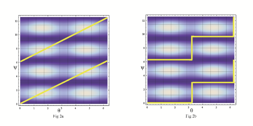
Figure 2: Figure 2a shows strings winding smoothly across the effective potential $\mathcal{V}$ on the $(\theta,\phi)$ sub-manifold. Figure 2b shows step-like configurations which minimises the total string energy within $\mathcal{V}$.

This leads to an apparent contradiction. We may assume, at the moment of loop formation, that $n\sim n_{\psi}\sim n_{\theta}\sim n_{\phi}>0$. After this point windings in the $\phi$-direction will still be able to vary smoothly, though they will not be stable and may in principle contract until they are point-like. This possibility is discussed in detail in section 5.6.

However, so long as $n_{\phi}>0$, windings in the ($\psi$, $\theta$) sub-manifold will relax into the step-like configuration shown in Figure 2b resulting in the formation of approximately $2n_{\psi}$ beads. This forces us to view the configuration as a series of small perturbations (in fact a series of $2n_{\psi}$ perturbations) away from a configuration described by $\psi=n\pi$ and $n_{\psi}=0$. We must therefore continue to regard $n_{\psi}>0$ (the number of windings in the $\psi$-direction at the moment of loop formation) as physically meaningful when estimating the number of beads, but we must regard it as approximately zero when estimating the bead mass. This is a little strange but it is quite consistent with the physical picture we have been sketching.

To obtain our estimate for the bead mass ($M_{b}$) therefore we first Taylor expand (4.3) with $n_{\psi}$ set equal to zero. Assuming $a_{0}r>>nR$ at the moment of loop formation, which corresponds to a large loop in the Minkowski directions, for all times we obtain the approximate expression,

$$V\sim\sqrt{1+\frac{\Pi^{2}}{T_{1}^{2}\lambda^{2}}}\left(2\pi a_{0}^{2}rT_{1}+T_{1}\int_{0}^{2\pi}d\sigma\frac{R^{2}\sin^{2}\psi(n_{\theta}^{2}+\sin^{2}\theta n_{\phi}^{2})}{r}\right)$$ (4.8)

We then move from the smooth windings picture shown in Figure 2a to the step-like configuration in Figure 2b by setting $\psi=m\pi$ globally, except in the vicinity of a bead where $\theta=m\pi$, $d\psi=d\sigma$ and $m\pi\leq\psi\leq(m+1)\pi$. Our expression for the total energy $V$ is then,

$$V\sim\sqrt{1+\frac{\Pi^{2}}{T_{1}^{2}\lambda^{2}}}\left(2\pi a_{0}^{2}rT_{1}+2n_{\psi}\times\frac{1}{2}T_{1}\frac{R^{2}}{r}n_{\theta}^{2}\int_{\psi_{i}=m\pi}^{\psi_{f}=(m+1)\pi}\sin^{2}\psi d\psi\right)$$

$$\sim\sqrt{1+\frac{\Pi^{2}}{T_{1}^{2}\lambda^{2}}}\left(2\pi a_{0}^{2}rT_{1}+2n_{\psi}\times\frac{\pi}{4}T_{1}\frac{R^{2}n_{\theta}^{2}}{r}\right).$$ (4.9)

As the first term is simply the rest mass of the string in the Minkowski directions, the second term corresponds to the rest mass of $N=2n_{\psi}$ beads. Finally, setting $n_{\psi}\sim n_{\theta}\sim n$ explicitly, we have the following estimates for both the initial number of beads $N$ and the bead mass $M_{b}$,

$$N\sim 2n$$

$$M_{b}\sim\frac{\pi}{4}T_{1}\sqrt{1+\frac{\Pi^{2}}{T_{1}^{2}\lambda^{2}}}\left(\frac{R^{2}n^{2}}{r}\right)$$ (4.10)

Note that the bead mass is inversely proportional to $r$. This makes sense on the assumption that the total length of the string remains constant. So if there is less string length involved in internal windings (resulting in less massive beads) more length is added to the ordinary four dimensional part of the loop. The converse is also true. Thus the first expression for the mass increases in magnitude as the second decreases and vice-versa. Note also that the $M_{b}$ is effectively quantised in terms of the number of windings present in the $\theta$-direction.

Let us now also consider the full expression for the bead mass. One can integrate the potential over the above range and the result is roughly the sum of the bead mass and the rest mass associated with an unwound string (with $n=0$). We can then re-write the bead mass including all the higher order terms, with an appropriate normalisation to yield

$$M_{b}\sim 2a_{0}^{2}T_{1}r\sqrt{1+\frac{\Pi^{2}}{T_{1}^{2}\lambda^{2}}}\left({\rm EllipticE}\left(\frac{nRi}{a_{0}r}\right)-\frac{\pi}{2}\right)$$ (4.11)

which is valid for non-zero winding number $n$. One can easily check that in the limit where $nR<<a_{0}r$ the mass reduces exactly to the one in (4.10).

5 Cosmological implications of necklace loops

We now investigate the cosmological implications of necklace loops based on the assumption that they retain their necklace structure after formation. As we have already seen, the $\theta$-dependence of the lifting potential depends on the presence of windings in the $\phi$-direction ($n_{\phi}>0$) and its $\psi$-dependence requires the presence of windings in the $\theta$-direction ($n_{\theta}>0$). However since the $\phi$-direction is flat, windings along this direction are unstable. If these windings contract this effectively flattens the $\theta$-direction leaving the $\theta$-windings free to contract as well. This in turn flattens the $\psi$-direction and necklace structure disappears as the bead mass (which comes from extra-dimensional windings) is converted into the ordinary rest mass of a loop in Minkowski space. We therefore see that, due to the presence of single flat direction in the $S^{3}$, the entire necklace structure of the loop is unstable and may unravel in time.

We will consider this possibility later in the present section where we will introduce a time-dependent model for the number of windings. For the moment we will we will consider $n\sim n_{\psi}\sim n_{\theta}\sim n_{\phi}$ to be roughly constant. We can now use Matsuda’s original assumption that the four-dimensional part of the loop loses mass-energy via the emission of gravitational radiation in Minkowski space (just like an ordinary cosmic string in four dimensions) but that the bead-mass which is formed from the winding of the string in internal space is unaffected by this process.

To investigate the cosmological implications of necklace loops we must therefore modify equation (4) by inserting a time-dependent radius $r(t,t_{i})$ into the first term of the expansion (the loop mass in Minkowski space) and the initial radius $r(t_{i})$ into the second term (the bead mass). The time dependent radius of a shrinking loop in warped Minkowski space is given by,

$$a_{0}r(t,t_{i})=a_{0}(\alpha t_{i}-\Gamma\mathcal{G}T_{1}(t-t_{i}))$$ (5.1)

where $t_{i}$ is the time of loop formation. Note that $t\geq t_{i}$ is the cosmic time coordinate, $\Gamma$ is a measure of the rate of energy loss due to the emission of gravitational radiation, $\mathcal{G}$ is Newton’s constant (which is determined by the volume of the $S^{3}$) and $0<a_{0}\alpha<a_{0}$ determines the characteristic initial loop radius as a fraction of the horizon, $d_{H}\sim a_{0}ct$ The initial loop radius as a function of $t_{i}$ is then

$$a_{0}r(t_{i})=a_{0}\alpha t_{i}.$$ (5.2)

The bead mass now explicitly depends on the time of loop formation, $t_{i}$ via (5.2). However we also expect the initial number of beads, $N$, will also depend in some way on $t_{i}$. We therefore need some way of estimating the initial number of windings in each direction $n=n(t_{i})$.

Following Shellard and Avgoustidis [12](and taking into account the warp factor $a_{0}$) we use the random walk regime to estimate the initial number of windings present in each angular direction, $n(t_{i})$, so that

$$n(t_{i})=\frac{\sqrt{a_{0}\alpha\omega_{l}\epsilon_{l}t_{i}}}{R}$$ (5.3)

where $0<\omega_{l}<1$ is the fraction of the total string length l (not to be confused with the angular momentum) contained in the windings and $\epsilon_{l}$ is the step length. This definition tells us that string networks will tend to form once the correlation length becomes larger than the scale of the internal dimensions.

The parameter $\omega_{l}$ may be defined as the ratio of the string length in the internal dimensions to the total length of the string in all dimensions. Following [12], but using the notation defined earlier, the concise definition of $\omega_{l}$ is given by

$$\omega_{l}=\sqrt{\int\left(\frac{R^{2}s^{\prime 2}}{a_{0}^{2}r^{2}+R^{2}s^{\prime 2}}\right)\mathcal{V}d\sigma/\int\mathcal{V}d\sigma}$$ (5.4)

where $\mathcal{V}(\sigma)$ denotes the integrand in equation (4.3). In order to simplify the above expression we then make the following approximations,

$$\omega_{l} \sim \sqrt{\frac{\int R^{2}s^{\prime 2}d\sigma}{\int(a_{0}^{2}r^{2}+R^{2}s^{\prime 2})d\sigma}\int\mathcal{V}d\sigma/\int\mathcal{V}d\sigma}$$ (5.5)

$$\sim \sqrt{\frac{n^{2}R^{2}\int(4+\sin^{2}(n\sigma)+\sin^{4}(n\sigma))d\sigma}{a_{0}^{2}r^{2}+n^{2}R^{2}\int(4+\sin^{2}(n\sigma)+\sin^{4}(n\sigma))d\sigma}}$$

where in the second step we have ignored the numerical coefficient in front of the $r^{2}$ term, and again used assumption that $n\sim n_{\psi}\sim n_{\theta}\sim n_{\phi}$. Finally we note that it is straightforward to show that

$$\int(4+\sin^{2}(n\sigma)+\sin^{4}(n\sigma))d\sigma\sim O(10)$$ (5.6)

for all possible values of $n(t_{i})$. Therefore we see that $\omega_{l}$ can be well approximated by the following function

$$\omega_{l}\sim\frac{nR}{\sqrt{a_{0}^{2}r^{2}+n^{2}R^{2}}}$$ (5.7)

up to various numerical factors which would have appeared in the above expression if the integral in (5.4) been performed in full. It is clear however, that $\omega_{l}$ has the correct functional dependence on both $n$ and $r$. This means that, whatever time-dependent models we use for $r(t_{i})$, $n(t_{i})$ and $\omega_{l}(t_{i})$ - they must satisfy (5.7) for consistency. Note that at this stage we are not imposing any additional conditions on $a_{0}r$ and therefore $\omega_{l}$ is just a parameter of the theory.

If we then use (5.2) as our model for $r(t_{i})$ and substitute $\omega_{l}$ from (5.7) into our previous expression for $n(t_{i})$ (which also uses the approximation $r(t_{i})\sim\alpha t_{i}$) we find a cubic equation in the variable $(nR)^{2}$,

$$(nR)^{6}+a_{0}^{2}(\alpha t_{i})^{2}(nR)^{4}-a_{0}^{2}(\alpha t_{i})^{2}\epsilon_{l}^{2}(nR)^{2}=0$$ (5.8)

This has the trivial solution $(nR)^{2}=0$ (no windings) and the more physically relevant one,

$$(nR)^{2}=\frac{a_{0}^{2}(\alpha t_{i})^{2}}{2}\left(-1\pm\sqrt{1+\frac{4\epsilon_{l}^{2}}{a_{0}^{2}(\alpha t_{i})^{2}}}\right)$$ (5.9)

although the reality of $n$ requires us to take the positive sign before the square root. The time dependence of $n(t_{i})$ in the expression above is then consistent with the definition of $\omega_{l}$ in (5.7).

Next we move on to consider to size of the step length $\epsilon_{l}$. The maximum velocity of the string in the compact dimensions is $c$ (where $c=1$ in natural units). which corresponds to a step length per unit time ($\Delta t=a_{0}^{-1}t_{s}=a_{0}^{-1}\sqrt{\alpha^{\prime}}$) of $\epsilon_{l}=a_{0}^{-1}l_{s}=a_{0}^{-1}\sqrt{\alpha^{\prime}}$. However only the endpoints of the string at the horizon move at the speed of light. For two points on the string within the horizon, separated by a distance $d\sim\alpha ct$, the relative velocity between them is $v\sim\alpha c$ which corresponds to an effective step length of,

$$\epsilon_{l}\sim\alpha a_{0}^{-1}\sqrt{\alpha^{\prime}}$$ (5.10)

Note that this definition also implies that $n(t_{i})\propto\alpha$ as we would expect. This ensures that the number of beads on a long string, which stretches across the entire horizon $n_{Hor}(t_{i})$, is independent of $\alpha$. In fact the assumption of a constant step length $\epsilon_{l}$ at all points along the string is problematic, as this leads to a measure of $n_{Hor}(t_{i})$ which is proportional to $1/\sqrt{\alpha}$.

Using (5.10) and (5.9) the condition for bead formation, $n(t_{i})^{2}\geq 1$, is then equivalent to,

$$t_{i}\geq\frac{R^{2}}{\alpha\sqrt{\alpha^{2}\alpha^{\prime}-a_{0}^{2}R^{2}}}$$ (5.11)

and reality of the above solution translates into the constraint

$$a_{0}^{2}\leq\frac{\alpha^{2}\alpha^{\prime}}{R^{2}}.$$ (5.12)

Now strictly speaking, $a_{0}^{2}$ is fixed by the ratio of the fluxes arising in a full string compactification and is therefore highly sensitive to the magnitude of string coupling, the string scale and the flux parameters. In the non-compact case which we are considering we also require that $a_{0}^{2}<1$ in order to ensure that the solution is warped. Therefore the existence condition for beads appears to impose a strict upper bound on the value of $a_{0}^{2}$ which in turn imposes a strong constraint on the deformation parameter of the conifold geometry. We also note that if $a_{0}^{2}=\frac{\alpha^{2}\alpha^{\prime}}{R^{2}}$, this allows necklaces to form only at infinity, and so only the strict inequality in (5.12) is physically meaningful.

One can now substitute the solution for $nR$ into the generalised mass function in (4.11). If we define the following function

$$G(t_{i})=-1+\sqrt{1+\frac{4\alpha^{\prime}}{a_{0}^{4}t_{i}^{2}}}$$ (5.13)

then we see that there is a remarkable cancellation of terms and we are left with

$$M_{b}\sim 2a_{0}^{2}T_{1}\alpha t_{i}\sqrt{1+\frac{\Pi^{2}}{T_{1}^{2}\lambda^{2}}}\left({\rm EllipticE}\left(i\sqrt{\frac{G(t_{i})}{2}}\right)-\frac{\pi}{2}\right)$$ (5.14)

which is not a monotonic function of time. For vanishingly small $t_{i}$ the mass is increasing until it reaches a maximum value, before decreasing monotonically. This leads to the interesting possibility that one can have sustained PBH formation during a small window where the mass function is greater than the critical value required to produce a gravitational radius larger than the string width. This possibility is dealt with explicitly in section 5.4.

We also note that the explicit form of $\omega_{l}(t_{i})$ is given by,

$$\omega_{l}\sim\frac{a_{0}^{2}t_{i}}{2\sqrt{\alpha^{\prime}}}\left(-1+\sqrt{1+\frac{4\alpha^{\prime}}{a_{0}^{4}t_{i}^{2}}}\right)=\frac{a_{0}^{2}t_{i}}{2\sqrt{\alpha^{\prime}}}G(t_{i})$$ (5.15)

which tends to unity as $t_{i}\rightarrow 0$ and zero as $t_{i}\rightarrow\infty$ as we would expect.

To aid visualisation in the discussions that follow we plot, in Figure 3, the functions $M_{b}(t_{i})$, $n(t_{i})$ and $\omega_{l}(t_{i})$ and the inter-bead distance $d(t_{i})$ for fixed values of our model parameters to illustrate the qualitative behaviour of each.

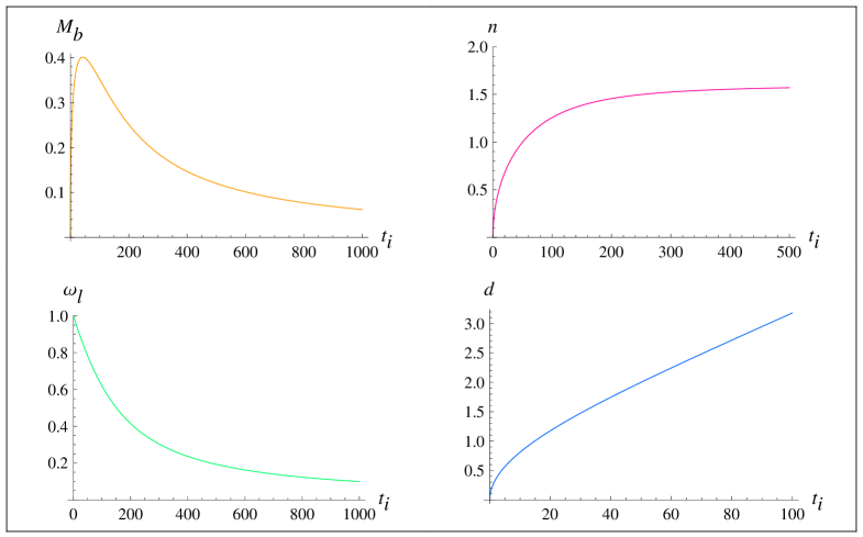
Figure 3: Plots of the mass of an individual bead $M_{b}$ as a function of time $t_{i}$, the number of beads $n(t_{i})$, $\omega_{l}(t_{i})$ and the average inter-bead distance $d(t_{i})$. In all plots model parameters have been set such that $a_{0}=0.1$, $\alpha^{\prime}=1$, $R=5$, $\alpha=0.8$ and $T_{1}\sqrt{1+\frac{\Pi^{2}}{T_{1}^{2}\lambda^{2}}}=1$.

What is clear from the plots is that, assuming no gravitational emission, there are initially few beads with large mass. However as time increases, the number density of beads gets larger and their corresponding mass decreases. The rate of decrease is in fact much larger than the increase in the number density. Therefore one expects that eventually the system will become dominated by a large number of (almost) massless beads.

5.1 Late time formation - the scaling regime

Using the fact that $nR$ is fixed by the parameters of the theory, let us consider the asymptotics to better understand the physics at early and late epochs. Let us initially focus on the late time regime where

$$t_{i}>>\frac{2\sqrt{\alpha^{\prime}}}{a_{0}^{2}}$$ (5.16)

which, using (5.9), implies that the initial number of beads is constant

$$n^{2}\sim\frac{\alpha^{2}\alpha^{\prime}}{a_{0}^{2}R^{2}}.$$ (5.17)

Note that the condition for bead formation $n(t_{i})^{2}\geq 1$ simply reproduces (5.12), ensuring the reality of $t_{i}^{(min)}$ - the minimum time at which necklaces formation begins - and is consistent with our expectations. We are then able to estimate the average inter-bead distance for necklaces formed at late times

$$d(t_{i})\sim\frac{a_{0}r(t_{i})}{N}\sim\frac{a_{0}^{2}Rt_{i}}{2\sqrt{\alpha^{\prime}}}.$$ (5.18)

Identifying this with the correlation length along the string, $L(t_{i})$, as mentioned in the previous section, we see that our solution corresponds to a scaling regime in which we may identify the scaling parameter $\gamma$ with the Klebanov-Strassler parameters, i.e.

$$d(t_{i})\sim L(t_{i})\sim a_{0}\gamma t_{i}$$ (5.19)

implying that,

$$\gamma\sim\frac{a_{0}R}{2\sqrt{\alpha^{\prime}}}$$ (5.20)

Compare this with the result of field theory calculations, where the initial number of beads on a loop of radius $r(t_{i})$ in the scaling regime is given by [16],

$$N(t_{i})\sim\frac{r(t_{i})}{L(t_{i})}\sim\frac{\alpha}{\gamma}$$ (5.21)

Hence we see that the condition for bead formation in the string picture (5.12) is equivalent to the condition for bead formation in the scaling regime of the field theory, $\gamma\leq\frac{1}{2}\alpha$. Both conditions ensure that $N\geq 2$, implying that beads come in pairs. This is also consistent with the identification of the inter-bead distance with degenerate vacuum states, or correlation distance, along the string. Thus we see that a scaling solution arises naturally at late times in the string picture allowing us to identify various string parameters with their field theory counterparts.

Using the condition on $\gamma$ and $\alpha$ which is consistent with bead formation i.e. $0<\gamma\leq\frac{1}{2}\alpha$, this simply recovers our previous constraint on $a_{0}R$ (5.12). However by setting $\alpha$ to the maximum value allowed by causality $\alpha=1$ we may place a maximum upper bound on the radius of the $S^{3}$

$$R\leq a_{0}^{-1}\sqrt{\alpha^{\prime}}.$$ (5.22)

This simply means that beads/windings will not form unless the radius of the $S^{3}$ is smaller than the warped string scale, irrespective of the value of $\alpha$. It also implies

$$a_{0}^{2}\leq\frac{1}{bMg_{s}}$$ (5.23)

in order for windings to form. Note also that setting $\epsilon_{l}\propto\alpha$ ensures that $n(t_{i})\propto\alpha$ even if $\omega_{l}$ is left as a free parameter as in [12]. Otherwise we have that $n(t_{i})\propto\sqrt{\alpha}$ which implies that the number of windings per Hubble volume is proportional to $1/\sqrt{\alpha}$ which seems unphysical.

We now ask what happens to the time dependence of the mass function in the late time limit. The argument of the EllipticE term becomes small and therefore we may series expand the mass term to obtain

$$M_{b}\sim T_{1}\sqrt{1+\frac{\Pi^{2}}{T_{1}^{2}\lambda^{2}}}\frac{\pi}{2}\frac{\alpha^{2}\alpha^{\prime\frac{3}{2}}}{a_{0}^{3}t_{i}}\left(1-\frac{3}{16}\frac{\alpha^{\prime}}{a_{0}^{4}t_{i}^{2}}+\ldots\right)$$ (5.24)

and therefore we see that the mass evolves inversely proportional to $t_{i}$ and that $M_{b}\to 0$ as $t_{i}\to\infty$. This implies that any necklace structure should disappear at sufficiently late times. In other words it is unlikely that any necklaces formed at late times would be distinguishable from ordinary string loops. One should quantify this by noting that the mass is also inversely proportional to the scale of the warping, therefore for highly warped throats the mass will be constant over a much larger time scale.

5.1.1 Early time formation

Returning now to the cubic solution for $(nR)^{2}$, let us consider early time formation subject to the condition that $t_{i}\leq\frac{2\sqrt{\alpha^{\prime}}}{a_{0}^{2}}$. This gives us

$$n^{2}(t_{i})\sim\frac{\alpha^{2}t_{i}\alpha^{\prime}}{R^{2}}-\frac{1}{2}\left(\frac{a_{0}}{R}\right)^{2}(\alpha t_{i})^{2}$$ (5.25)

to second order, which also implies that,

$$\omega_{l}(t_{i})\sim 1-\frac{1}{2\sqrt{\alpha^{\prime}}}a_{0}^{2}t_{i}$$ (5.26)

from the definition of $\omega_{l}$. Clearly therefore $\omega_{l}\rightarrow 1$ as $t_{i}\rightarrow 0$, that is as $a_{0}r(t_{i})\rightarrow\mathcal{O}(nR)$. Utilising the bead-formation condition then allows us to place a bound on the bead formation time via

$$\frac{R^{2}}{\alpha\sqrt{\alpha^{2}\alpha^{\prime}-a_{0}^{2}R^{2}}}\leq t_{i}\leq\frac{2\sqrt{\alpha^{\prime}}}{a_{0}^{2}}.$$ (5.27)

The average distance between beads, should necklaces begin to form., may then be approximated by

$$d(t_{i})\sim\frac{a_{0}R\sqrt{t_{i}}}{2\alpha^{\prime 1/4}}\left(1+\frac{a_{0}^{2}t_{i}}{4\sqrt{\alpha^{\prime}}}+\ldots\right)$$ (5.28)

which, unlike the the late time approximation, does not correspond to any known regime in the field theory if we continue to identify $d(t_{i})$ with the correlation distance $L(t_{i})$. However we note that the second term is sub-dominant at very early times when $t_{i}\leq\frac{4\sqrt{\alpha^{\prime}}}{a_{0}^{2}}$ suggesting that it may be reasonable to keep only first order terms in the expansion especially if $t_{i}<<\frac{2\sqrt{\alpha^{\prime}}}{a_{0}^{2}}$. Such a very early time approximation may correspond to a damping regime in the field theory picture. The above equation would then represent an intermediate regime where damped and scaling solutions can be joined together. Assuming now that $t_{i}<<\frac{2\sqrt{\alpha^{\prime}}}{a_{0}^{2}\alpha}$ and keeping only the first order term in (5.25), we see that the condition for bead formation $n^{2}(t_{i})\geq 1$ is then equivalent to,

$$t_{i}\geq\frac{R^{2}}{\alpha^{2}\sqrt{\alpha^{\prime}}}$$ (5.29)

This is consistent with our previous estimates and shows that bead formation will occur in the very early time regime only when $a_{0}^{2}R^{2}<<\alpha^{2}\alpha^{\prime}$. With this in mind we see that the inter-bead distance is set by the leading factor in (5.28) which is consistent with the field theory picture at early times during the damping regime, where we expect the correlation distance $L(t_{i})$ to be given by a power law solution of the form [16],

$$L(t_{i})\sim t_{d}^{\frac{1}{2}}t_{i}^{\frac{1}{2}}$$ (5.30)

with $t_{d}$ corresponding to the characteristic damping time of small scale oscillations on the string.

However a damping regime is usually obtained by considering collisions of the string with an external plasma. In this case the damping term comes from the internal dynamics of the model, suggesting that the inertia of the beads (when $M_{b}$ is large) is sufficient to cause the correlation length to scale as $L(t_{i})\sim\sqrt{t_{i}}$ at very early times.

Furthermore unless the warping is extraordinarily large, the time-scales over which this effect takes place are likely to be insignificant in cosmological terms. As a future amendment to the current work therefore it will be useful to impose an external damping regime and to study the effect of the interaction of the windings with the external plasma. Naively we may expect collisions of the string with particles in the compact space to inhibit the formation of windings resulting in the delayed on-set of a scaling regime. This to is likely to mirror the field theory case, though further investigation is needed to establish whether the correlation distance scales according to (5.30).

Once again, for the sake of completeness, we consider how the mass function changes as a function of time in this epoch. The elliptic integral is actually divergent in this limit, however we can consider the leading order divergence which will dominate the spectrum. The resulting expression for the mass function will then behave like

$$M_{b}\sim 2T_{1}\sqrt{a_{0}\alpha^{\prime 1/4}}\sqrt{1+\frac{\Pi^{2}}{T_{1}^{2}\lambda^{2}}}(\alpha t_{i})^{3/4}$$ (5.31)

which one can see will tend to zero as $t_{i}$ goes to zero. This is within the regime where we expect PBH formation to occur, since the mass of the necklace plus beads is steadily increasing (as a function of time) during this regime.

5.2 PBH formation

We now calculate the contribution to the PBH mass spectrum from collapsing necklace loops, based on the assumption that loops which chop off from the string network retain their necklace structure indefinitely. We will initially take the number of beads per loop to be constant from the time of formation.

The minimum radius to which a contracting loop may shrink, $\delta_{l}$, is limited by the string width - which we assume to be comparable to the inverse of the symmetry breaking scale $\eta_{s}$ [15, 20], i.e. $\delta_{l}\sim\eta_{s}^{-1}$ . The condition for gravitational collapse then becomes

$$R_{S}>\eta_{s}^{-1}$$ (5.32)

where $R_{S}$ is the Schwarzschild radius of the loop. We may estimate the Schwarzschild radius of a necklace loop using the spherically symmetric approximation

$$R_{S}(t_{i})\sim 2\mathcal{G}M_{T}(t_{i})$$ (5.33)

where $\mathcal{G}$ is the modified Newton’s constant and $M_{T}(t_{i})$ is the total mass of the necklace. A necklace formed at time $t_{i}$ will therefore collapse to form a PBH if,

$$M_{T}(t_{i})\geq\frac{\eta_{s}^{-1}}{2\mathcal{G}}$$ (5.34)

Assuming that $\delta_{l}$ is small, the bead mass will provide the dominant contribution to $M_{T}(t_{i})$ so that

$$M_{T}(t_{i}) \sim N(t_{i})M_{b}(t_{i})$$ (5.35)

$$\sim \frac{8T_{1}a_{0}^{3}}{\sqrt{2}R}\sqrt{1+\frac{\Pi^{2}}{T_{1}^{2}\lambda^{2}}}(\alpha t_{i})^{2}\sqrt{G(t_{i})}\left({\rm EllipticE}\left(i\sqrt{\frac{G(t_{i})}{2}}\right)-\frac{\pi}{2}\right)$$

which is not a monotonic function. We can approximate the solution at early and late time regimes respectively using the following

$$M_{T}(t_{i}) \sim T_{1}\sqrt{1+\frac{\Pi^{2}}{T_{1}^{2}\lambda^{2}}}\frac{\pi}{4}\frac{\alpha^{2}\sqrt{\alpha^{\prime}}}{R}a_{0}t_{i}+\ldots$$ (5.36)

$$\sim T_{1}\sqrt{1+\frac{\Pi^{2}}{T_{1}^{2}\lambda^{2}}}\frac{\pi}{2}\frac{\alpha^{2}\alpha^{\prime\frac{3}{2}}}{a_{0}^{3}R}\frac{1}{t_{i}}\left(1-\frac{3\alpha^{\prime}}{16a_{0}^{4}t_{i}^{2}}\right)$$

Here we note that $M_{T}$ is linearly increasing with $a_{0}t_{i}$ at very early times, whilst in the late time epoch we find that the scaling is with $1/(a_{0}^{3}t_{i})$. Thus the sensitivity to the warp factor is most pronounced at late times, since a vanishingly small value of $a_{0}$ means that the total mass remains larger over a wider time-scale. Ultimately however, the total mass will tend to zero asymptotically. The complete mass function $M_{T}(t_{i})$, using the definition of the elliptic integral, is sketched in Figure 4 to illustrate the time dependence. In Figure 5 this is shown together with the early and late time time approximations.

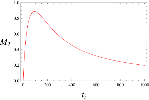
Figure 4: The total mass $M_{T}$ contained within the beads of a necklace as a function of $t_{i}$. The model parameters have been fixed so that $a_{0}=0.1$, $\alpha=0.8$, $\alpha^{\prime}=1$, $T_{1}\sqrt{1+\frac{\Pi^{2}}{T_{1}^{2}\lambda^{2}}}=1$ and $R=5$.

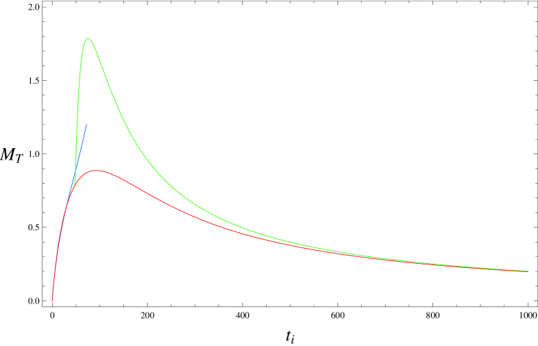
Figure 5: The total mass $M_{T}$ contained within the beads of a necklace as a function of $t_{i}$, together with the early and late time approximations given in equation $(\ref{eq:early_late_approx})$. The same parameter choices were made as in Fig. 4. The blue (green) curves are the early (late) time approximations respectively. Note that the late time approximation seems to over-estimate the maximum mass.

Without precise values for the model parameters it is difficult to determine the accuracy (as a percentage estimate) of either the early or late time approximations. However it is interesting to note that the late time approximation also qualitatively captures the behaviour of $M_{T}(t_{i})$ in the early time regime. In fact the peaks of the two functions are in approximately the same position, although the peak of the approximation is roughly twice as high as the peak of the true curve.

However it is also clear that the peak of the full mass function, which is potentially the region of greatest interest with respect to the formation of PBH’s, lies between the regions in which either the early or late time approximations are valid. As we shall see, in order to calculate the PBH spectrum analytically in terms of our model parameters, we must integrate over the region of the curve (5.35) which satisfies (5.34). This is not possible in general, as any such region (if it exists) will certainly include the peak itself. We must therefore find some way of approximating the elliptic integral in this crucial region.

Whilst this can be done in many ways, we will use the following method. To begin with, we estimate the maximum height of the full mass function by utilising the fact that the peak of the late time approximation lies at roughly the same value of $t_{i}$. Differentiating the second equation in (5.36) and solving the resulting expression $dM_{T}/dt_{i}=0$ gives,

$$t_{i}^{(peak)}\sim\frac{3}{4a_{0}^{2}}$$ (5.37)

Substituting this back into (5.35) then gives,

$$M_{T}^{(peak)}=M_{T}(t_{i}^{(peak)})\sim 5.47\ T_{1}\sqrt{1+\frac{\Pi^{2}}{T_{1}^{2}\lambda^{2}}}\frac{\alpha^{2}\alpha^{\prime\frac{3}{2}}}{8a_{0}R}$$ (5.38)

We then note that substituting the full expression for $n(t_{i})$ (5.9) into (4.10) and using $M_{T}(t_{i})\sim N(t_{i})M_{b}(t_{i})$ from (5.35) also gives a function which shows the same qualitative behaviour as the true $M_{T}(t_{i})$ curve (as we would expect). Taking this approach corresponds to expanding the elliptic integral only to first order in $n(t_{i})$, but keeping the full time dependence of this function (which is valid even at early times) as opposed to keeping higher order terms in the expansion of the elliptic integral and using the late time approximation $n(t_{i})\sim\alpha\sqrt{\alpha^{\prime}}/a_{0}R$ as in (5.36). The resulting expression for $M_{T}(t_{i})$ is,

$$M_{T}(t_{i})\sim\frac{\pi}{\sqrt{32}}T_{1}\sqrt{1+\frac{\Pi^{2}}{T_{1}^{2}\lambda^{2}}}\frac{a_{0}^{3}(\alpha t_{i})^{2}}{R}\left(-1+\sqrt{1+\frac{4\alpha^{\prime}}{a_{0}^{4}t_{i}^{2}}}\right)^{\frac{3}{2}}$$ (5.39)

Although this is still highly inaccurate within the region of the peak, a function of this form may be used to capture the behaviour of the full expression right down to all but the earliest times (where the early time expansion above must again be used).. We may then fit a curve of the form,

$$M_{Tapprox}(t_{i})\sim A\ T_{1}\sqrt{1+\frac{\Pi^{2}}{T_{1}^{2}\lambda^{2}}}\frac{a_{0}^{3}(\alpha t_{i})^{2}}{R}\left(-1+\sqrt{1+\frac{C\alpha^{\prime}}{a_{0}^{4}t_{i}^{2}}}\right)^{\frac{3}{2}}$$ (5.40)

where $A$ and $C$ are free parameters, to the true $M_{T}(t_{i})$ curve by demanding the approximate function satisfies;

• to pass through the point $(t_{i}^{(peak)},M_{T}^{(peak)})=\left(\frac{3}{4a_{0}^{2}},5.47\ T_{1}\sqrt{1+\frac{\Pi^{2}}{T_{1}^{2}\lambda^{2}}}\frac{\alpha^{2}\alpha^{\prime\frac{3}{2}}}{8a_{0}R}\right)$ and,

• to have the same asymptotic behaviour as as the full elliptic integral. This is equivalent to the requirement that $A=\frac{\pi}{\sqrt{32}}C^{-\frac{3}{2}}$.

These two condition are sufficient to fix $A$ and $C$ uniquely giving,

$$A \rightarrow 0.368657$$

$$C \rightarrow 5.25648$$ (5.41)

The resulting fit is remarkably good both at late times and in the vicinity of the peak and is shown for a selection of parameter values in Figure 6 below. Only at very early times does the approximation appear to break down, which becomes clear if we ’zoom in’ near $t_{i}=0$ as shown in Figure 7. However, if we are required to integrate over a time range that includes a region in which $M_{Tapprox}(t_{i})$ given in (5.40) becomes invalid, we may always split the resulting integral into two parts. It would then be necessary to integrate, using the early time approximation in (5.36) and expanded to arbitrary order, over some range $0\leq t_{i}\leq t_{E}$ (where $t_{E}$ marks the time at which the approximation starts to break down) - whilst using the expression (5.40)/(5.2) over the remainder of the range $t_{E}\leq t_{i}\leq t_{F}$.

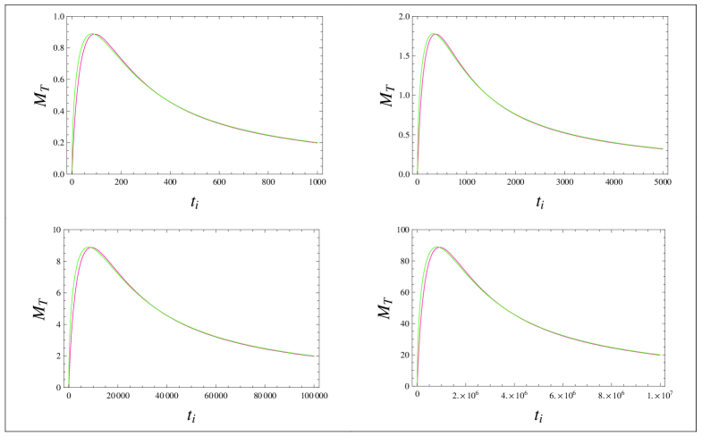
Figure 6: Plot of the exact Necklace mass $M_{T}$ (red curve) and the approximate fit function $M_{Tapprox}$ (green curve)as a function of $t_{i}$ for $a_{0}=0.1,0.05,0.01,0.001$ (top left to bottom right). In all the plots $\alpha^{\prime}=1$, $R=5$, $\alpha=0.8$ and $T_{1}\sqrt{1+\frac{\Pi^{2}}{T_{1}^{2}\lambda^{2}}}=1$.

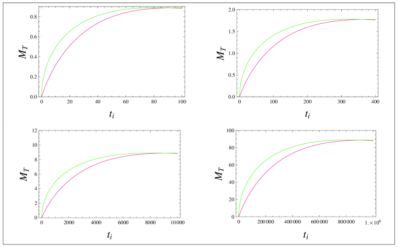
Figure 7: Zoom in of the four plots shown in Figure 6 clearly exhibiting the early time breakdown of the fit function $M_{Tapprox}(t_{i})$

Starting with (5.32) we may now estimate the range of time over which necklaces will form, that will eventually collapse to produce black holes i.e necklaces with sufficiently high mass contained in their beads to produce a Schwarzschild radius greater than the string width. From our previous discussion we see that the mass function peaks at earlier times, therefore favouring PBH formation in this regime - that is, from the collapse of small necklace loops with a relatively low number of high mass beads.

In fact it is clear from $N(t_{i})$, $M_{b}(t_{i})$ in Figure 3, and especially from the plot $M_{T}(t_{i})\sim N(t_{i})M_{b}(t_{i})$ in Figure 4, that the increase in bead number at late times is insufficient to compensate for the reduction in the mass of individual beads. Similarly at very early times, there are an insufficient number of extra-dimensional windings to produce enough beads to create a large Schwarzschild radius, even though the individual bead mass is high. This results in the formation of a window in the early universe, during which necklaces suitable for the formation of PBH’s are produced.

The limits of this window, let us call them $t_{PBH}^{\pm}$, may be estimated by solving equation (5.34) with the appropriate expression for $M_{T}(t_{i})$. Let us now assume that the energy scale of the symmetry breaking process which gives rise to the $(p,q)$ string network is equal to the un-warped string energy scale,

$$\eta_{s}\sim\sqrt{\alpha^{\prime}}^{-1}$$ (5.42)

and consider the limits which arise from inserting (5.40) with the values of A and C given above. The resulting time bounds can be solved for analytically but yield rather complicated expressions which we do not repeat here.

These analytic expressions are valid so long as the equation(5.40) provides a relatively good approximation to the true $M_{T}(t_{i})$ curve. However the validity of the lower bound, $t_{PBH}^{-}$, should always be checked (for a given set of parameter values) by plotting the full mass function together with the PBH formation bound,

$$\frac{\eta_{s}^{-1}}{2\mathcal{G}}\sim\frac{R^{3}(\alpha^{\prime})^{2}}{2}\frac{1}{G_{(10)}}$$ (5.43)

where we have used the fact that the effective four-dimensional gravitational coupling is related to the ten dimensional one through the relation

$$\mathcal{G}=\frac{G_{(10)}}{\rm{Vol}(X_{6})},$$ (5.44)

where $X_{6}$ is the internal manifold. We can approximate the coupling via

$$\mathcal{G}\sim\frac{G_{(10)}}{R^{3}(\alpha^{\prime})^{3/2}}$$ (5.45)

although we will typically assume that $G_{(10)}\sim\mathcal{O}(1)$ (in units where $\alpha^{\prime}=1$) for simplicity. In the event that this forms a poor estimate of the true $t_{PBH}^{-}$ it is necessary to expand the early time approximation given in (5.36) to as many orders as required to reach an accurate value and to re-solve (5.34).

For the sake of completeness we note that the early time expansion given to first order, as in (5.36), remains reasonably accurate up to,

$$t_{E}\sim\frac{\sqrt{\alpha^{\prime}}}{2a_{0}^{2}}$$ (5.46)

beyond which the function (5.40) is undoubtedly valid. The resulting estimate of $t_{PBH}^{-}$ (where $t_{PBH}^{-}<t_{E}\sim\frac{\sqrt{\alpha^{\prime}}}{2a_{o}^{2}}$) is,

$$t_{PBH}^{-}\sim\frac{R^{4}}{8a_{0}{\alpha^{\prime}}^{5/2}\alpha^{2}T_{1}\sqrt{1+\frac{\Pi^{2}}{T_{1}^{2}\lambda^{2}}}}$$ (5.47)

In order to be safe therefore we may choose to split up any integral involving the the necklace mass $M_{T}(t_{i})$ into two pieces: the first using the early time approximation (5.36) between the limits $t_{PBH}^{-}\leq t_{i}\leq t_{E}$ and the second part using (5.40) between $t_{E}\leq t_{i}\leq t_{PBH}^{+}$ where $t_{E}$ is given by (5.46).

An estimate for $t_{PBH}^{+}$ can also be obtained using the late time expansion for $M_{T}(t_{i})$ and this yields the simple expression:-

$$t_{PBH}^{+}\sim\frac{\pi{\alpha^{\prime}}^{7/2}\alpha^{2}T_{1}\sqrt{1+\frac{\Pi^{2}}{T_{1}^{2}\lambda^{2}}}}{a_{0}^{3}R^{4}}$$ (5.48)

The next step towards calculating the necklace contribution to the present day PBH spectrum is to estimate the time at which a collapsing loop reaches its minimum radius $\delta_{l}\sim\eta_{s}^{-1}\sim\sqrt{\alpha^{\prime}}$. This depends on the time the loop formed $t_{i}$ via

$$t^{\prime}(t_{i})\sim\left(1+\frac{\alpha}{\Gamma\mathcal{G}T_{1}}\right)t_{i}-\frac{\eta_{s}^{-1}}{\Gamma\mathcal{G}T_{1}}.$$ (5.49)

We expect, from our approximations, that $\delta_{l}$ will be small and therefore the second term will be sub-dominant. This implies that the corresponding time range over which PBH’s actually form from the collapse of these loops is given by ${t^{\prime}}_{PBH}^{-}\leq t^{\prime}(t_{i})\leq{t^{\prime}}_{PBH}^{+}$ where

$${t^{\prime}}_{PBH}^{\pm}\sim\left(1+\frac{\alpha}{\Gamma\mathcal{G}T_{1}}\right){t}_{PBH}^{\pm}.$$ (5.50)

The initial mass of a black hole forming at $t^{\prime}(t_{i})$ is therefore equal to $M_{T}(t_{i})$, which can be compared with the mass of black holed formed from ordinary string loops - $M_{PBH}(t_{i})\sim\mu\alpha t_{i}$, which yields the present day mass spectrum [38]

$$\frac{dn_{PBH}(M)}{dM}\propto M^{-2.5}.$$ (5.51)

Clearly the mass spectrum for black holes formed via the collapse of necklaces is far more complicated, although the relevant calculation of the present day spectrum proceeds in a similar fashion. Firstly we identify

$$M_{PBH}(t^{\prime}(t_{i}))=M_{T}(t_{i})$$ (5.52)

Assuming also that the PBH formation window lies in the radiation dominated epoch, the number density of string loops with initial length $r(t_{i})=\alpha t_{i}$ which chop off from the network at time $t_{i}$ is given by,

$$n(r(t_{i}),t_{i})\sim\frac{\nu_{r}}{t_{i}^{\frac{3}{2}}(r(t_{i}))^{\frac{3}{2}}}=\frac{\nu_{r}}{\alpha^{\frac{3}{2}}t_{i}^{3}}$$ (5.53)

where $\nu_{r}$ is the number of long strings per Hubble volume. Now in field theoretic models,

$$\nu_{r}=g\gamma^{-3}\tilde{c}$$ (5.54)

where $g$ is a Lorentz factor, $\gamma$ gives the correlation length as a fraction of the horizon (which we previously identified with the string theory parameters $\gamma\sim\frac{a_{0}R}{2\sqrt{\alpha^{\prime}}}$ (5.20)) and $\tilde{c}$ is the loop production parameter. For ordinary four-dimensional strings $\tilde{c}$ is extracted from simulations and is of order unity. For higher dimensional strings $\tilde{c}$ is suppressed by a factor $P$ given by,

$$P\sim\left(\frac{\delta}{R}\right)^{d-3}$$ (5.55)

where $\delta$ is the effective string thickness and $d$ is the number of spatial dimensions. In our model $\delta\sim\eta_{s}^{-1}\sim\sqrt{\alpha^{\prime}}$ and $d=6$ giving,

$$P\sim\left(\frac{\sqrt{\alpha^{\prime}}}{R}\right)^{3}$$ (5.56)

and hence,

$$\nu_{r}\sim\frac{8g}{a_{0}^{3}}\left(\frac{\sqrt{\alpha^{\prime}}}{R}\right)^{6}$$ (5.57)

In higher dimensional theories the scaling parameter $\gamma$ (which determines the correlation length) is also expected to be suppressed by a factor of $P$ during the scaling regime, but small scale structure on the strings is likely to lead to weaker $P$-dependence, $P_{\rm{eff}}=f(P)$ [14, 12]. However as the correlation length has already been determined directly in terms of the model parameters it is likely that this effect has already been accounted for. We also note that it appears consistent in the warped geometry to account for the warping of both space and time by introducing the transformations $t_{i}\rightarrow a_{0}t_{i}$, $r(t_{i})\rightarrow a_{0}r(t_{i})$ into the expression (5.53) above, yielding an additional factor of $a_{0}^{-3}$. However it is our belief that this effect is already accounted for via the derivation of $\nu_{r}$ in terms of the warped throat model parameters. In fact such an explanation gives a nice interpretation to the formula (5.57) which is then seen as the product of three terms: a ”warping term” which accounts for the back-reaction on the large dimensions $a_{0}^{-3}$, a term accounting for extra-dimensional effects $(\sqrt{\alpha^{\prime}}/R)^{3}$ and a standard Lorentz factor $\sim g$.

The formation rate of black holes at $t^{\prime}(t_{i})$ is then equivalent to (minus) the rate of necklace formation at $t_{i}$,

$$\frac{dn_{PBH}(t^{\prime}(t_{i}))}{dt^{\prime}(t_{i})}=-\frac{dn(r(t_{i}),t_{i})}{dt_{i}}\sim\frac{3\nu_{r}}{\alpha^{\frac{3}{2}}t_{i}^{4}}$$ (5.58)

and finally we may use the the fact that

$$\frac{dn_{PBH}(t^{\prime}(t_{i}))}{dM_{PBH}(t^{\prime}(t_{i}))} = \frac{dn_{PBH}(t^{\prime}(t_{i}))}{dt^{\prime}(t_{i})}\times\frac{dt^{\prime}(t_{i})}{dM_{PBH}(t^{\prime}(t_{i}))}$$ (5.59)

$$\sim \frac{3\nu_{r}}{\alpha^{\frac{3}{2}}t_{i}^{4}}\times\left(\frac{dM_{T}(t_{i})}{dt_{i}}\right)^{-1}$$

to find the contribution to the PBH mass-spectrum from collapsing necklaces by substituting for $t^{\prime}(t_{i})$ and red-shifting to the current epoch.

Of more interest for us is the calculation of the total contribution of the spectrum to the fraction of the critical density of the universe in the current epoch, $\Omega_{PBH}(t_{0})$. The standard formula for $\Omega_{PBH}(t_{0})$ from collapsing cosmic string loops is [20]

$$\Omega_{PBH}(t_{0})=\frac{1}{\rho_{crit}(t_{0})}\int_{max(t_{c},t_{*})}^{t_{0}}dt\frac{dn_{PBH}}{dt}M(t,t_{0})$$ (5.60)

where $t_{*}$ is the formation time of a black hole with mass $M_{*}\approx 4.4\times 10^{14}h^{-0.3}$ gm ($\equiv 10^{20}$ in Planck units), whose lifetime would be the present age of the universe. $M(t,t_{0})$ is the current mass of a black hole that formed at a time $t$, and $t_{c}$ is the time at which loops first begin to form.

Again assuming that most of the loop production occurs in the radiation dominated era, the rate of black hole formation is then given by

$$\frac{dn_{PBH}}{dt}=\frac{3\nu_{r}f}{\alpha^{\frac{3}{2}}t^{4}}\frac{a(t)^{3}}{a(t_{0})^{3}}$$ (5.61)

where $f$ is the fraction of loops which collapse on the first oscillation, which is expected to be small. It is typical to neglect the effect of Hawking radiation by making the approximation $M(t,t_{0})\sim M(t)$, which in the standard case ($M(t)\sim\mu Gt$) has been shown to make a difference of less than $6$ per cent to the final value of $\Omega_{PBH}(t_{0})$ [38].

Adjusting the standard calculations to account for the effect of necklace formation, we expect there to be contributions to $\Omega_{PBH}(t_{0})$ from two qualitatively different sources: Firstly we expect to find a spike in the formation of PBH’s in the very early universe due to the gravitational collapse of necklace loops which shrink to their minimum radius $\delta_{l}\sim\eta_{s}^{-1}$ within a time $t^{\prime}\sim\left(1+\frac{a_{0}\alpha}{\Gamma\mathcal{G}T_{1}}\right)t_{i}$, although on cosmological time scales we may simply assume $t^{\prime}\sim t_{i}$. The total mass of all the beads contained in these loops is large, and is therefore the dominant contribution to the initial mass of the black hole. This corresponds to the first term in (5.2) below.

The second contribution to $\Omega_{PBH}(t_{0})$ comes from loops which collapse before shrinking to their minimum size, by adopting a sufficiently compact and spherically symmetric configuration on their first oscillation [16]. In principle this process is continuous through the history of the universe, although at late times we may neglect the contribution of the beads to the masses of black holes formed in this way - leaving just the first term in the second integral. At early times the beads must be included and therefore both terms become important.

The expression for the (approximate) contribution of PBH’s formed from collapsing loops to the current mass-density of the universe is therefore

$$\Omega_{PBH}(t_{0})\approx\frac{1}{\rho_{crit}(t_{0})}\int_{t_{*}^{-}}^{t_{*}^{+}}dt_{i}\frac{3\nu_{r}}{\alpha^{\frac{3}{2}}t_{i}^{4}}\frac{a(t_{i})^{3}}{a(t_{0})^{3}}M_{T}(t_{i})\times\left(\frac{t_{*}^{+}}{t_{r}}\right)^{\frac{1}{2}}\left(\frac{t_{r}}{t_{0}}\right)^{\frac{3}{2}}$$

$$+\frac{1}{\rho_{crit}(t_{0})}\int_{t_{*}^{+}}^{t_{0}}dt_{i}\left(\frac{6\pi\nu_{r}fT_{1}\sqrt{1+\frac{\Pi^{2}}{T_{1}^{2}\lambda^{2}}}}{\alpha^{\frac{1}{2}}t_{i}^{3}}+\frac{3\nu_{r}fM_{T}(t_{i})}{\alpha^{\frac{3}{2}}t_{i}^{4}}\right)\frac{a(t_{i})^{3}}{a(t_{0})^{3}}$$ (5.62)

where $t_{*}^{\pm}$ are the times between which the necklace mass exceeds $M_{*}$ and $t_{r}$ marks the end of the radiation dominated era. In practice however the factor $f\sim 10^{-20}$ multiplying the integral on the second line indicates that (without fine tuning of the parameters) by far the largest contribution will come from the first integral between $t_{*}^{-}$ and $t_{*}^{+}$. In other words we expect the necklace-specific channel to dominate the production of PBH’s and therefore choose to neglect the latter two terms.

The two factors in large brackets outside the first integral account for the red-shifting from the end of PBH production (with $M_{PBH}\geq M_{*}$) from necklace collapse to the present day. For our purposes it is convenient to use the parameterisation

$$\rho_{crit}(t_{0})\sim 3H_{0}^{2}M_{p}^{2},\hskip 14.22636ptt_{0}\sim\frac{2}{3}H_{0}^{-1}.$$ (5.63)

Note that for PBH’s to form via the necklace-specific process outlined above and to survive to the present day, thus contributing to the current mass density of the universe, we require

$$M_{T}(t_{i})\geq M_{*}$$ (5.64)

for at least some range of $t_{i}$ within $t_{PBH}^{-}\leq t_{i}\leq t_{PBH}^{+}$. There are then three possible scenarios which we can consider.

• $M_{*}\leq\frac{\eta_{s}^{-1}}{2\mathcal{G}}$ If this condition is satisfied for all $t_{i}$ in which black holes are produced, we can integrate the first term in (5.2) over the range $t_{PBH}^{-}\leq t_{i}\leq t_{PBH}^{+}$.

• $\frac{\eta_{s}^{-1}}{2\mathcal{G}}<M_{*}<M_{T}^{(max)}$ With $M_{*}$ in this range, the expression above will automatically be satisfied for times between $t_{*}^{-}\leq t_{i}\leq t_{*}^{+}$, which may be obtained by solving (5.64).

• $M_{*}>M_{T}^{(max)}$ All PBH’s formed by this process will evaporate long before the present epoch.

In reality the first of these scenarios will not occur if $\eta_{s}\sim\sqrt{\alpha^{\prime}}^{-1}\ (\equiv M_{Pl})$ unless $R$ is hierarchically larger than the fundamental string scale. This is theoretically compatible with the bound (5.12) for small enough values of the warp factor, though we need not assume that the bound is close to saturation. Working in Planck units and using the values for $\mathcal{G}$ (5.44) and $\eta_{s}$, it is possible to show that $M_{*}>\eta_{s}^{-1}/2\mathcal{G}$ so we need only ’tune’ the values of our model parameters so that $M_{T}(t_{i})>M_{*}$ for at least some range of $t_{i}$. It turns out that the most important parameters for ensuring this condition is met are the warp factor $a_{0}$ and the world-sheet flux momentum $\Pi$. There is in fact a region (if somewhat restrictive) of the whole parameter space of $a_{0},R,\Pi$ for which this condition is met which we shall discuss later. But it seems that one is either required to have small values of $a_{0}$ and/or large values of $\Pi$. That large $\Pi$ should help ensure PBH production is understandable since the pre-factor $\sqrt{1+\frac{\Pi^{2}}{T_{1}^{2}\lambda^{2}}}$ simply multiplies the expression for $M_{T}(t_{i})$, whereas increasing world-sheet flux does not affect the value of $M_{*}$. However the relation between $M_{T}(t_{i})$ and $a_{0}$ is more complicated as this factor appears in a complex way inside the Elliptic function.

For the sake of completeness we calculate $t_{*}^{\pm}(M_{*})$ explicitly by setting $M_{T}(t_{i})=M_{*}$. We then use the early time expansion of $M_{T}(t_{i})$, given previously, to estimate $t_{*}^{-}$ - and the late time approximation to $M_{T}(t_{i})$ to obtain $t_{*}^{+}$. The result is

$$t_{*}^{-}(M_{*}) \sim \frac{M_{*}R}{4T_{1}a_{0}\alpha^{2}T_{1}\sqrt{1+\frac{\Pi^{2}}{T_{1}^{2}\lambda^{2}}}}\alpha^{\prime-\frac{1}{2}}$$

$$t_{*}^{+}(M_{*}) \sim \frac{\pi\alpha^{2}T_{1}\sqrt{1+\frac{\Pi^{2}}{T_{1}^{2}\lambda^{2}}}}{2a_{0}^{3}M_{*}R}\alpha^{\prime\frac{3}{2}}$$ (5.65)

Although one could also obtain $t_{*}^{+}$ by equating $M_{Tapprox}(t_{i})$ with $M_{*}$, the resulting expression for $t_{*}^{+}$ is rather unwieldy and does not significantly differ in its value from the approximate form given here. The evaluation of $\Omega_{PBH}(t_{0})$ (5.2) between the limits $t_{*}^{-}$-$t_{*}^{+}$ (given by (5.2) above) is then obtained by integrating between $t_{*}^{-}$ and $t_{E}$ using the early time approximation (5.46) and between $t_{E}$ and $t_{*}^{+}$ using the numerical fit. The full expression is then well approximated by the following:

$$\Omega(t_{0})\sim$$

$$\frac{10^{-25}g\sqrt{\alpha}\sqrt{\Pi^{2}+\lambda^{2}T_{1}^{2}}}{\pi a_{0}R^{7}t_{0}^{3/2}\rho_{crit}}[-4AC^{\frac{1}{4}}(F-1)^{-\frac{1}{4}}\left\{\frac{F+5}{(F-1)^{\frac{1}{4}}}-3\times 2^{\frac{3}{4}}\,{{}_{2}F_{1}}\left(\frac{1}{4},\frac{1}{4};\frac{5}{4};\frac{1}{2}(1-F)\right)\right\}$$

$$-(2{\left(\frac{32}{\pi}\right)}^{\frac{1}{2}}(F^{2}-1)^{-\frac{1}{4}}-\frac{1}{384}(\rm{Log}(256)-3)(F^{2}-1)^{\frac{3}{4}}+\sqrt{2\pi}(1+\rm{Log}(16))(F^{2}-1)^{\frac{1}{4}}$$

$$-\pi\rm{Log}\left(\frac{1}{8a_{0}}(F^{2}-1)^{\frac{1}{2}}\right)-8\pi\rm{Log}\left(\frac{1}{2a_{0}^{2}}\right)-19.312)]$$ (5.66)

where ${}_{2}F_{1}$ is the usual Hypergeometric function and we have defined $F=F(a_{0},R,M_{*},\alpha,\lambda T_{1},\Pi)$ to be;

$$F=\frac{16a_{0}^{2}M_{*}^{2}R^{2}}{\alpha^{4}(\Pi^{2}+\lambda^{2}T_{1}^{2})}.$$ (5.67)

As noted above, the fulfillment of the condition $M_{T}(t_{i})\geq M_{*}$ requires small values of the warp factors and/or large values of the flux parameter $\Pi$ - though the exact relationship between $M_{T}(t_{i})$ and $a_{0}$ is complex. We must also ensure, for consistency, that $t_{*}^{-}(M_{*})<t_{*}^{+}(M_{*})$ (where these values are given by the expression (5.2)). Exactly how small $a_{0}$ is required to be in order to fulfill both of these requirements depends on how large we take the $\Pi$ to be. We see from the explicit expression for $\Pi$ given below that, in principle, $0\leq\Pi\leq\infty$ for flux $\lambda F_{0\sigma}$ in the allowable range $0\leq\lambda^{2}F_{0\sigma}^{2}\leq a_{0}^{2}(a_{0}^{2}r^{2}+R^{2}s^{\prime 2})$.

$$\Pi=\frac{2T_{1}\lambda^{2}F_{0\sigma}^{2}}{a_{0}^{2}\sqrt{r^{2}+a_{0}^{-2}R^{2}s^{\prime 2}-a_{0}^{-4}\lambda^{2}F_{0\sigma}^{2}}}$$ (5.68)

As causality requires that $F_{0\sigma}^{2}<a_{0}^{4}\lambda^{-2}(r^{2}+a_{0}^{-2}R^{2}s^{\prime 2})$ we may assume,

$$F_{0\sigma}^{2}=\beta a_{0}^{4}\lambda^{-2}(r^{2}+a_{0}^{-2}R^{2}s^{\prime 2})$$ (5.69)

where $0\leq\beta<1$. Equation (5.68) may then be re-written in terms of $\beta$ so that,

$$\Pi=\frac{2T_{1}\sqrt{\beta}\lambda}{\sqrt{1-\beta}}$$ (5.70)

from which it is clear that $\beta=0$ corresponds to $\Pi=0$ and that $\Pi\rightarrow\infty$ as $\beta\rightarrow 1$. However the bound for PBH formation is not the only condition we must consider as the predictions of our model must also be consistent with observational bounds. Current observational constraints on the energy density of PBH’s come from the EGRET experiment, which measures the extra-galactic gamma ray flux at 100MeV [27]. By calculating the expected contribution to this flux from black holes expiring at the present epoch [38, 39] (see also [40] for bounds derived for the standard PBH spectrum using the latest data) they were able to show that the current density of PBH’s formed via the collapse of cosmic strings is bounded by

$$\Omega_{PBH}(t_{0})<10^{-9}.$$ (5.71)

Note however that this bound is based on the prediction that the PBH mass spectrum follows the profile predicted by the standard Hawking collapse process, such that $M_{PBH}(t)\sim t$ and the number density per mass interval is given by (5.51). Technically one should recalculate this bound using the spectrum predicted by the necklace-specific collapse channel in order to place bounds on the model parameters from experimental data. We hope to supply a re-calculated bound on $\Omega_{PBH}(t_{0})$ at a later date, but content ourselves for the time being with $\Omega_{PBH}(t_{0})<10^{-9}$ as a ”ball park” figure with which to proceed.

With this in mind we see that not all the region of parameter space allowing PBH production is compatible with observation. For example, ’typical’ values of $a_{0}\sim 10^{-11}$ and $\Pi\sim 10^{12}$ are sufficient to ensure that $M_{T}(t_{i})>M_{*}$ for at least some $t_{i}$ but the resulting value of the $\Omega_{PBH}(t_{0})$ integral (5.2)is huge ($\Omega_{PBH}(t_{0})\sim 10^{3}>>1$) if $R$ is comparable to the string scale. However due to the large $R$-dependence in the denominator caused by the extra-dimensional contribution to $\nu_{r}$ we (happily) see that typical values of $R\sim 10^{2}$ are sufficient to bring $\Omega_{PBH}(t_{0})$ within the observable bound $\Omega_{PBH}(t_{0})<10^{-9}$. Thus the dimensions of the compact space need not be hierarchically larger than the string scale in order for the predictions of our model to be consistent with observational constraints.

To systematically explore the values of $a_{0},R$ and flux $\Pi$ which are consistent with all the constraints above, we can express the value of the peak of the necklace mass function, $M_{Tapprox}$ given earlier in (5.40), in terms of $M_{*}$;

$${M_{T}}^{peak}\sim 5.47\ T_{1}\sqrt{1+\frac{\Pi^{2}}{T_{1}^{2}\lambda^{2}}}\frac{\alpha^{2}\alpha^{\prime\frac{3}{2}}}{8a_{0}R}=\kappa M*$$ (5.72)

where $\kappa>1$ is a parameter that for given values of $(a_{0},\alpha,R,\Pi,T_{1},\alpha^{\prime})$ express how far the peak value of $M_{T}$ is above the mass scale $M_{*}$. Using this definition we can expresses the quantity $\sqrt{1+\frac{\Pi^{2}}{T_{1}^{2}\lambda^{2}}}$ in terms of $(a_{0},\alpha,R,\kappa,T_{1},\alpha^{\prime})$ and the above terms for $t_{*}^{\pm}$ simplify considerably

$$t_{*}^{-}=\frac{0.171{\alpha^{\prime}}^{-1/2}}{a_{0}^{2}T_{1}\kappa},\qquad t_{*}^{+}=\frac{2.297T_{1}\kappa{\alpha^{\prime}}^{3/2}}{a_{0}^{2}}$$ (5.73)

It is interesting to note that both $t_{*}^{-}$ and $t_{*}^{+}$ depend on the warp factor as $a_{0}^{-2}$. It may be thought that for $\kappa=1$, the times $t_{*}^{-}$ and $t_{*}^{+}$ should approach one another since the definition of $t_{*}$ requires values of $t_{i}$ for which $M_{T}=M_{*}$. However recall we have assumed the early time approximation for $M_{T}$ in determining $t_{*}^{-}$, and not the ’late-time’ approximation $M_{Tapprox}$. This assumption then requires that we take $\kappa>1$. We could of course consider situations where $\kappa$ is closer to unity, but then one has to use $M_{Tapprox}$ in the determination of both $t_{*}^{-}$ and $t_{*}^{+}$ - which is technically complicated.

Now evaluating (5.2) using the above, we obtain an expression that depends on the parameters $(a_{0},\alpha,R,\Pi,T_{1},\alpha^{\prime},t_{0},\rho_{crit})$. In Figure 8 we present a contour plot showing the values of $R,\kappa$ that are consistent with the condition $\Omega_{PBH}(t_{0})<10^{-9}$. In this plot we have taken, as a typical value, $\alpha=0.8$ and have set $T_{1}=\alpha^{\prime-1}=1$ and input the standard values of $\rho_{crit}$, $t_{0}$ and $M_{*}$. The resulting bounds on $\{R,\kappa\}$ are remarkably insensitive to the actual value of $a_{0}$ because the latter only appears in $\Omega_{PBH}(t_{0})$ via logarithmic factors.

For given (allowed) values of $\{R,\kappa\}$ we can then deduce the value for the flux parameter $\Pi$ via (5.72), which is of course sensitive to the value of $a_{0}$.

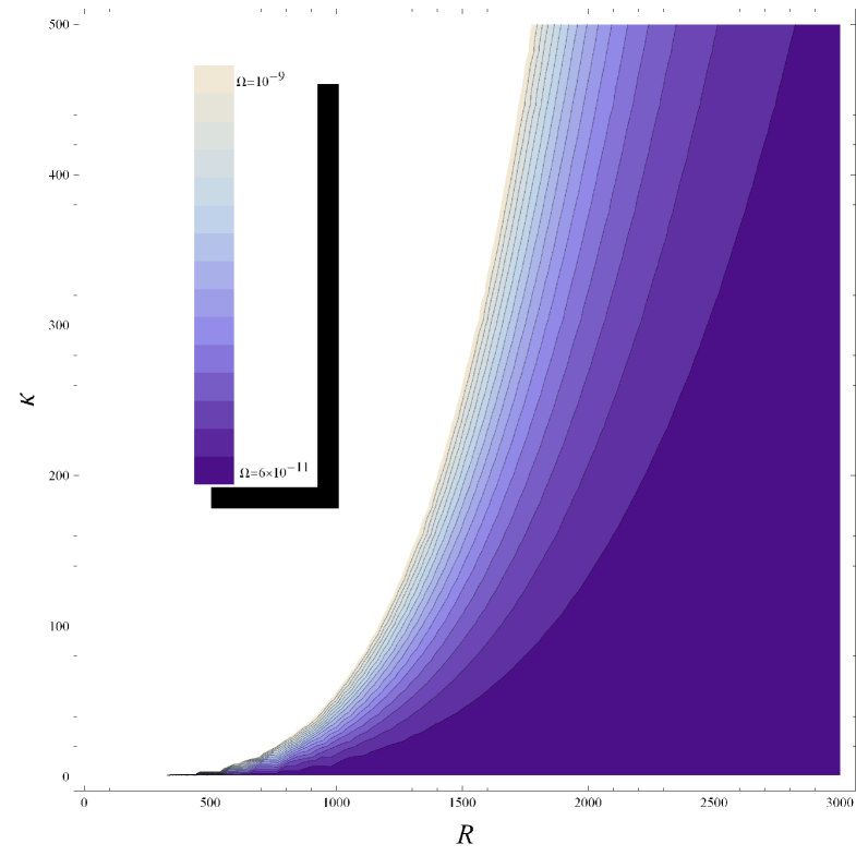
Figure 8: Contour plot showing the allowed regions of $\{R,\kappa\}$ consistent with the bound $\Omega(t_{0})<10^{-9}$. Only a few contours are plotted. We have chosen $a_{0}=0.1,T_{1}=1=\alpha^{\prime}$ and $\alpha=0.8$

To visualize the allowed values of the flux parameter $\Pi$ corresponding to those of $a_{0},R,\kappa$ - we use a 3D-contour plot shown in Figure 9. We illustrate six typical surfaces in the $\{\rm{Log}[a_{0}],R,\kappa\}$ plane corresponding to values of $\Pi=10^{12},10^{10},10^{8},10^{6},10^{4},10^{2}$ (from front to back). These surfaces also take into account the observational allowed values of $\{R,\kappa\}$ illustrated in Figure 8.

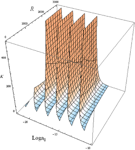
Figure 9: 3D Contour plots showing values of the flux parameter $\Pi$ in the ($\rm{Log}[a_{0}],R,\kappa$) plane. Six surfaces are shown corresponding (from front to rear) to the values of $\Pi=10^{12},10^{10},10^{8},10^{6},10^{4},10^{2}$. These plots take into account the observational bounds on ${R,\kappa}$ shown in Figure 8. The remaining choice of parameters are as in Figure 8.

5.3 Quasi-stable necklaces

Let us now drop the assumption that the loops retain their necklace structure indefinitely. As outlined earlier, it is reasonable to expect that wrappings in the flat $\phi$-direction may unwind over time leading to a ”flattening” of the $\theta$-direction. This in turn flattens the $\psi$ direction and, so on until the whole necklace structure unravels.

Assuming that the motion of the string in the $\phi$-direction remains random after the formation of a loop, and that the motion is also random in any newly flattened direction, we should expect the characteristic lifetime of the beads in any necklace to be comparable to the formation time, $t_{i}$. This is because the average warped time taken for a single $\phi$-winding to contract to a point is $a_{0}t_{1}\sim\frac{R^{2}}{a_{0}^{-1}\sqrt{\alpha^{\prime}}}$ - where this is the time associated with a single winding . The warped time taken for $n(t_{i})$ such windings to contract is therefore

$$a_{0}t_{n(t_{i})}\sim\frac{n^{2}(t_{i})R^{2}}{a_{0}^{-1}\sqrt{\alpha^{\prime}}}$$ (5.74)

As we are only considering that part of the string which forms the extra-dimensional windings we may compare the expression above with (5.3) in which $\omega_{l}$ and $\alpha$ have been set to unity. We then see that,

$$t_{n(t_{i})}\sim t_{i}$$ (5.75)

This implies that the number of necklaces originally formed at $t_{i}$ which survive for a time $\Delta t>>t_{i}$ after formation will be negligible, with most having become standard string loops. However it is difficult to estimate the fraction of necklaces surviving for an arbitrary length of time $\Delta t$ using such generic arguments, though this is exactly what we must calculate to determine the true contribution of necklace collapse to the PBH mass spectrum. In particular we must calculate the fraction of loops which retain their necklace structure for an interval $\Delta t\sim\frac{\alpha}{\Gamma\mathcal{G}T_{1}}t_{i}$. To do this we consider the probability distribution which describes fluctuations of the radial coordinate. For a random walk this is simply a Gaussian distribution with mean $\mu=0$ and variance,

$$\sigma^{2}(\Delta t)\sim a_{0}^{-1}\frac{\Delta t}{\delta t}\epsilon_{l}^{2}\sim a_{0}^{-2}\sqrt{\alpha^{\prime}}\Delta t$$ (5.76)

where $\delta t\sim a_{0}^{-1}\sqrt{\alpha^{\prime}}$ is the time interval between steps, $\epsilon_{l}\sim a_{0}^{-1}\sqrt{\alpha^{\prime}}$ is the step length and $\Delta t$ is the total (un-warped) time elapsed. The total probability density function $\Phi(t,\sigma(\Delta t))$ is given below.

$$\Phi(t,\sigma(\Delta t)) \sim \frac{1}{\sqrt{2\pi}\sigma(\Delta t)}e^{-\frac{1}{2}\frac{t^{2}}{\sigma^{2}(\Delta t)}}$$ (5.77)

$$\sim \frac{a_{0}}{\sqrt{2\pi}(\sqrt{\alpha^{\prime}}\Delta t)^{\frac{1}{2}}}\exp\left(-\frac{a_{0}^{2}t^{2}}{2\sqrt{\alpha^{\prime}}\Delta t}\right).$$

Since a loop forming at time $t_{i}$ has $n(t_{i})$ windings to lose, the radial coordinate must ”travel” a distance approximately equal to $n(t_{i})R$ in order for the loop to lose its necklace structure. The fraction of necklaces $f(\Delta t)$ which survive for an interval $\Delta t$ after $t_{i}$ is then given by the integral of the above expression between $t\sim\pm a_{0}^{-1}n(t_{i})R\sim\pm a_{0}^{-1}\left(\sqrt{\alpha^{\prime}t_{i}}\right)^{\frac{1}{2}}\sim\pm\sigma(t_{i})$ which can be well approximated using the error function

$$f(\Delta t) \sim Erf\left(\frac{\sigma(t_{i})}{\sqrt{2}\sigma(\Delta t)}\right)\sim Erf\left(\frac{1}{\sqrt{2}}\frac{a_{0}^{-1}\left(\sqrt{\alpha^{\prime}t_{i}}\right)^{\frac{1}{2}}}{a_{0}^{-1}\left(\sqrt{\alpha^{\prime}\Delta t}\right)^{\frac{1}{2}}}\right)$$ (5.78)

$$\sim Erf\left(\sqrt{\frac{t_{i}}{2\Delta t}}\right).$$

Thus when $\Delta t\sim t_{i}$ the fraction of loops which have retained their extra-dimensional windings is approximately

$$f(t_{i})\sim Erf\left(\frac{1}{\sqrt{2}}\right)\sim 0.68$$ (5.79)

which matches well with our result (5.75) . The fraction of necklaces which survive until they reach the minimum radius is,

$$f\left(\Delta t\sim\frac{\alpha}{\Gamma\mathcal{G}T_{1}}t_{i}\right)\sim Erf\left(\frac{1}{\sqrt{2}}\left(\frac{\alpha}{\Gamma\mathcal{G}T_{1}}\right)^{-\frac{1}{2}}\right)$$ (5.80)

Strictly speaking therefore the integral (5.2) should be multiplied by the additional numeric factor above to account for the the loss of necklaces which un-ravel before reaching the point at which they can undergo gravitational collapse.

We also note that $f\left(\Delta t\sim\frac{\alpha}{\Gamma\mathcal{G}T_{1}}t_{i}\right)\leq 10^{-20}$ when,

$$\alpha\geq 1.591\times 10^{39}\Gamma\mathcal{G}T_{1}$$ (5.81)

and thus the necklace-specific channel becomes comparable (or sub-dominant) to the standard Hawking process. Practically however the values of $\alpha$, $\Gamma$, $\mathcal{G}$ and $T_{1}$ here are such that this is unlikely to occur without significant fine tuning.

5.4 Comparison with the standard string-monopole network

The dynamics of string-monopole network evolution depends crucially upon the ratio of the monopole energy density to the string tension [17, 15]. This dimensionless parameter, denoted $\mathcal{R}$ in the literature is given by,

$$\mathcal{R}=\frac{m}{\mu d}$$ (5.82)

where $m$ is the the monopole mass, $\mu$ is the tension and $d$ is the distance between monopoles. For $\mathcal{R}<<1$ the network behaves like an ordinary string network - reaching a scaling solution at late times, but for $\mathcal{R}>>1$ the mass of the beads dominates the dynamics of the evolution. In our case these energy scales are time dependent and the corresponding parameter is given by

$$\mathcal{R}(t_{i})=\frac{M_{b}(t_{i})}{T_{1}d(t_{i})}$$ (5.83)

which scales as $\mathcal{R}\sim t_{i}^{-2}$ for $t_{i}>>\frac{2\sqrt{\alpha^{\prime}}}{a_{0}^{2}\alpha}$ and $\mathcal{R}\sim t_{i}^{-\frac{1}{2}}$ for $t_{i}<<\frac{2\sqrt{\alpha^{\prime}}}{a_{0}^{2}\alpha}$. Thus we see that as $t_{i}\to\infty$ we find $\mathcal{R}\to 0$ and vice-versa. Our results are therefore consistent with the standard analysis in that the necklaces behave like an ordinary string network for $\mathcal{R}<<1$ but like a string-monopole network when $\mathcal{R}>>1$ since the mass of the beads becomes significant.

However the dynamics of $\mathcal{R}$ differ profoundly in our model. This indicates that the effect of beads formed from extra-dimensional windings is different to the effect created by monopoles with regard to network evolution. To understand this in more detail let us consider the latter. The standard equation for the evolution of $\mathcal{R}$ is [41],

$$\frac{\dot{\mathcal{R}}}{\mathcal{R}}=-\kappa_{s}t^{-1}+\kappa_{g}t^{-1}$$ (5.84)

where the first term on the right hand side describes the stretching of the string due to the cosmic expansion and the the second term describes the contraction due to emission of gravitational radiation. It is a reasonable to assume that

$$\kappa=\kappa_{g}-\kappa_{s}>0$$ (5.85)

which allows us to solve (5.84), up to some constant of integration,

$$\mathcal{R}\sim t^{\kappa}.$$ (5.86)

Using (5.82) the evolution of the inter-monopole distance then scales like

$$d\sim\mathcal{R}^{-1}\sim t^{-\kappa}.$$ (5.87)

This was the crucial assumption Matsuda used to identify $d(t)$ with the step length of the random walk $\chi(t)$ [41] of the monopole along the string. From this point, the estimated initial number of beads per loop is then given by

$$n(t_{i})\sim\frac{r(t_{i})}{d(t_{s})\times\left(\frac{t}{t_{s}}\right)^{k-1}}$$ (5.88)

where $d(t_{s})\sim(t_{M}t_{s})^{\frac{1}{2}}$ is the initial bead spacing in the network at the time of string formation $t_{s}$ (where here $t_{s}\sim\sqrt{\alpha^{\prime}}$) and $k=0$ corresponds to the (natural) $\kappa=1$ solution of (5.84).

Assuming that $\sim\sqrt{n}$ beads would survive without annihilation, we find that $m_{coil}\propto\sqrt{n}$ and hence,

$$m_{coil}\sim t_{i}^{\frac{2-k}{2}}$$ (5.89)

which favours black hole production at late times vs dark matter production for small $t_{i}$. This is the standard result assuming that necklaces which reach their minimum radius but which have insufficient mass to undergo collapse to form PBH’s can only interact with other matter gravitationally, leading to the production of Planck scale dark matter relics. In Matsuda’s original scenario however, based on the assumptions above, large numbers of Planck scale dark matter ’particles’ are formed at early times with smaller numbers of increasingly massive black holes formed at later times. In our model this process is essentially reversed with a window of PBH production in the early universe (though potentially this window may be quite large for small $a_{0}$ so the last epoch of PBH formation is not necessarily ’early’, even on cosmological time scales) when $M_{T}(t_{i})>M_{*}$ with dark matter forming well into the scaling regime when $M_{T}(t_{i})<M_{*}$.

Physically the above equations describe the shrinking of the string sections connecting neighbouring monopoles. Effectively the contraction of the string is able to pull these monopoles through the horizon at an ever increasing rate . Hence we find that the early and late time limits of $\mathcal{R}$ as defined above, are the opposite of those obtained from (5.83), namely that $\mathcal{R}\to\infty$ as time increases, whilst tending to zero as $t_{i}\to 0$.

Similarly the natural solution, $\kappa=\kappa_{g}-\kappa_{s}\sim 1$ obtained from an order of magnitude estimate, gives $d\sim t^{-1}$ in the standard case as opposed to $d\sim t$ in our case. In yet another respect therefore we have obtained the opposite results to the standard analysis.

However it is not immediately obvious that what applies to monopoles formed in a separate phase transition also applies to beads formed by extra-dimensional windings. Although a contracting string may pull ordinary monopoles through the horizon at an ever increasing rate, a winding may not cross the horizon ready-made and concentrated at a point from a four-dimensional perspective. This is because insufficient time will have elapsed to establish correlations in the compact dimensions. Put another way, if the horizon advances by a distance $a_{0}c\delta t$, the end point of the string formerly localised at the horizon, can move by, at most, a distance $c\delta t$ from its original position in the compact space. Causality therefore places a limit on the rate at which new windings can enter the horizon, whereas no such limit exist for ordinary monopoles .

In fact the considerations above help to explain why the number of windings $n(t_{i})$ is proportional to the ratio $a_{0}/R$ not simply to $R^{-1}$ in the warped throat model. Although larger $R$ results in a slower rate of winding formation (as we would expect) this effect is, at least potentially, dwarfed by the effect of the warp factor $a_{0}$ (c.f. (5.17)) which is related to $R$ via the deformation parameter, $a_{0}^{2}\sim\tilde{\epsilon}^{\frac{4}{3}}R^{-2}$ This is because $a_{0}$ limits the increase of the horizon distance in the infinite directions (but not in the compact space) via

$$d_{H}(\delta t)=a_{0}c\delta t$$ (5.90)

As the resultant velocity of the end point of the string is $c=1$ smaller $a_{0}$ results in a greater velocity in the compact spaces and hence a larger limiting value for $n(t_{i})$.

In general however, windings may enter the horizon more rapidly the smaller their effective radii. In fact this at least partially accounts for the falling bead mass at late times; since $t_{i}\rightarrow\infty$ we expect that $\omega_{l}\rightarrow 0$ for a random walk in the extra dimensions. This could be achieved through either;

• Falling number density (per unit distance along the string) at late times - $n\sim d^{-1}$

• Windings wrapping ever smaller effective radii in the $S^{3}$

The fact that $d^{-1}\sim t_{i}^{-1}$ at late times highlights the first effect and $M_{b}\sim t_{i}^{-1}$ indicates the second. In practice however we would expect both effects to play some role.

The question then arises, does the shrinking bead mass have a counterpart in field theory? We may also consider whether the arguments for the limitation of windings entering the horizon hold true for field-theoretic strings in the dual non-Abelian Higgs models.The present authors hope to address this question in a future publication.

Finally we note that the predictions of our model (specifically that PBH production is favoured at early times with dark matter production at later epochs, in contrast to previous predictions) are highly dependent on the assumption of a random walk regime which produces the extra-dimensional windings. It is not immediately clear how this behaviour might be modified by the introduction of a velocity correlations regime, though it is possible that the results may be more in line with those of previous studies. This is a question the authors hope to pursue at a later date. It is also highly dependent upon the assumption that only beads formed from net windings, not from bead-anti-bead ($b-\bar{b}$) pair formation, contribute to the mass of PBH’s/DM relics. As we have seen, assuming that $\sim\sqrt{n}$ $b$/$\bar{b}$’s survive until the string reaches it’s minimum radius (where $n$ here must be taken to include all beads/anti-beads created from random steps along the string, not simply those formed by net displacement in the compact space) leads to (5.89) and to qualitative behaviour which is the very opposite to that obtained in our model. However as stated previously in the footnote on page 15, we believe that such an argument is valid only for a static string and that in a contracting loop all $b$’s will eventually collide with their $\bar{b}$ counterparts before the minimum radius is reached. In particular, in our model we may expect the initial $b-\bar{b}$ spacing to be approximately equal to the step length $\epsilon_{l}\sim a_{0}^{-1}\alpha\sqrt{\alpha^{\prime}}$ which is most certainly greater that the minimum radius $\delta_{l}\sim\eta_{s}^{-1}\sim\sqrt{\alpha^{\prime}}$ for all reasonable values of $\alpha$ and $a_{0}$.

6 Discussion

In this note we have investigated a simple cosmic string model using several key ideas from string theory. Our starting point was the assumption that there is some initial stage of inflation that leads to the creation of trapped strings (along the lines of [7]) that have non-zero windings in the internal space. We argued that the string feels a lifting potential due to the non-trivial geometry of the background, forming a ‘kinky cycloop’. By estimating the mass of such a string configuration we were able to show that formation at late times reduces to a scaling solution, which one may hope to identify with a relic dark matter phase. We also note in passing that, in principle, we require dark matter production from necklaces between $t_{PBH}^{+}$ and $t_{0}$ not to over-close the universe. However, as the present day dark matter density bound is approximately $\Omega_{DM}(t_{0})<0.3$ and due to the $t^{-3}$ suppression of the loop production function, we find that in all but pathological cases the PBH density bound $\Omega_{PBH}(t_{0})<10^{-9}$ is by far the most stringent constraint.

In some sense this has been a bottom up approach to the problem. The warp factor is simply a parameter of the metric, depending only on the extra-dimensional flux and the deformation parameter of the (non-compact) supergravity background. A fully realised UV approach will precisely fix the warping as a function of the closed string moduli VEV’s and the flux, therefore leading to a more tightly constrained theory. However we would hope that the general features of our approach will remain intact. In particular the formation window for PBH at early times contrasts strongly with the field theory/string model proposed by Matsuda. Although the authors initially feared that result may be in some sense disappointing, due to the likelihood of PBH’s formed at early times having evaporated by the present epoch, we have shown that it is possible within the model here constructed to satisfy the condition $M_{T}(t_{i})>M_{*}$ and current observational constraints. It is worth noting too at this point that, for very small $a_{0}$, the window of black hole formation may be sufficiently large for the assumption of a constant $M_{*}$ to become inaccurate. A more detailed analysis would therefore take into account the rate of black hole evaporation in the extra-dimensional background introducing a time-dependent lower bound on the PBH mass $M_{*}(t_{i})$. An improved analysis would also consider how the abundance of PBH’s formed through necklace collapse in the very early universe affects BBN and subsequent structure formation. In fact, there are many theoretical and observational constraints which any such model must satisfy concurrently, thereby potentially allowing the Klebanov-Strassler model parameters to be bounded with even greater precision.

It is clear from our model that in order to generate any PBH’s of mass $M_{*}$ restricts us to a small region of the $(a_{0},R,\Pi)$ parameter space as is shown by in Figures 8 and 9. This is not surprising if we recall that $M_{*}\sim 10^{20}$ in Planck units and so there is a hierarchy issue here. On the other hand since the warp factor $a_{0}$ depends exponentially on background fluxes, obtaining small enough values to generate a hierarchically large $M_{T}$ is perhaps not so unnatural.

In order to satisfy the PBH observational bounds one requires larger background flux $M$ if there is larger world-volume flux $\Pi$. This is inherently obvious, since the additional world-volume flux can be treated as an effective mass correction to the necklace. This additional mass will back-react on the solution and the probe limit will be rendered invalid, unless the background flux is also increased to compensate. What is interesting is that, for fixed warping, there is a large parameter space where bounds are satisfied. Another interesting feature is that, as is clear from Figure 8, the allowed values of $R$ for regions where $M_{T}>>M_{*}$ (corresponding to large $\kappa$) are still in the ’mild’ hierarchy region $R\sim 10^{3}l_{s}$. Indeed the only way to have a value of $R\sim l_{s}$ and consistent with observation requires a fine tuning where the peak of $M_{T}$ is taken very close to but just above $M_{*}$. This then reduces the time interval of mass $M_{*}$ PBH formation given by $(t_{*}^{-}-t_{*}^{+})$ which can be made small enough so that we can reduce the value of $R$ and still obtain $\Omega_{PBH}(t_{0})<10^{-9}$.

Our construction is very model dependent in some sense, since it is only valid for a special class of supergravity backgrounds of the type IIB string. Another interesting class of cosmic string models arises from considering Heterotic M-theory on the orbifold $CY_{3}\times S^{1}/\mathbb{Z}_{2}$. The strings in this case can arise from wrapping membranes (or five-branes) over various cycles within the internal space [42, 43]. Topologically stable strings are only possible for five-branes wrapping a complete four-cycle within the CY space [44]. However, other wrappings are potentially possible if there is an uplifting potential and a similar analysis can be performed. We leave this for a future publication.

One other issue that remains is the validity of substituting the expression $r(t_{i})=\alpha t_{i}$ for the variable $r$ in the bead mass terms of the EllipticE expansion and $r(t,t_{i})=\alpha t_{i}-\Gamma T_{1}\mathcal{G}(t-t_{i})$ into the leading order term representing the mass of the four-dimensional sections of the string. As stated previously, this is entirely consistent with Matsuda’s original assumption that the bead mass remains constant after loop production due to the ”trapping” effects of the lifting potential, whereas the sections of string not contained in the extra-dimensional windings shrink through the emission of gravitational radiation. However, the re-paramaterisation invariance of the Nambu-Goto action implies that it may not be possible to talk of one ’section’ of the string expanding/contracting while other sections remain fixed. By definition strings have no sub-structure which would seem to imply that they must expand or contract along their entire length. In our model this would mean that the contraction of the string due to gravitational radiation in the warped Minkowski directions in fact produces a contraction of the string along the internal direction as well. If true this implies that the expression $r(t,t_{i})$ should be substituted in both the bead-mass and four-dimensional parts of the string mass integral, thus creating an explicitly time dependent bead-mass $M_{b}(t,t_{i})$ for $t>t_{i}$. Potentially this may alter the present results significantly, as we would expect the number of necklaces which retain sufficient mass in their extra-dimensional windings to produce PBH’s when reaching their minimum radius to diminish sharply. This is therefore likely to lead to a much smaller amount of black hole production and greatly increased dark matter formation. It is hoped that the question of the explicit time dependence of the bead mass may be resolved conclusively by investigating field theory duals of the string necklaces discussed here. Again, the present authors hope to be able to offer some contribution in this direction in the near future.

A further aside concerns the question of binding energy between $b-b$ or $\bar{b}-\bar{b}$ pairs which coalesce. In field theoretic models the binding energy between true monopole or anti-monopole pairs may be calculated. We may suspect that, if a similar binding energy exists between beads formed from extra-dimensional windings, it’s presence may alter the string dynamics so that the evolution of a string configuration with $n$ ’one step’ beads into a single bead formed from $n$ steps will be energetically favoured. Once formed it is also possible that such a configuration may un-wind more rapidly than it’s corresponding $n$-bead counterpart, leading to a necessary modification of the arguments in Section 5.3. As a first approximation we have assumed that there is no binding energy between winding states. In the absence of a full BSFT picture this seems intuitively likely, given that the string must be considered as a collective phenomenon, which suggests that the unwinding of $n$ single steps will be just as hard as un-winding a single $n$-step wrapping. However it is not clear how one can really understand this problem without a more detailed analysis of the boundary theory.

Finally it is interesting to speculate further on the recent result implied by the PAMELA experiment [45, 46] which suggests that there is an over-abundance of high energy positrons in the cosmic background. Rather than interpreting this as a signal for dark matter, it has also been suggested that this is in agreement with predictions from cosmic-strings [47]. It would certainly be interesting to extend our analysis along those lines.

Acknowledgments

We wish to thank Levon Pogosian for a useful discussion. M.L is supported by an STFC studentship and the Queen Mary EPSTAR consortium. This work was supported in part by NSERC of Canada. Thanks also to the referee for their clarifying remarks.

We dedicate this work to the memory of David Birtles.

References

- [1] E. Komatsu et al. [WMAP Collaboration], arXiv:0803.0547 [astro-ph].
- [2] J. K. Adelman-McCarthy et al. [SDSS Collaboration], Astrophys. J. Suppl. 162, 38 (2006) [arXiv:astro-ph/0507711].
- [3] E. J. Copeland, R. C. Myers and J. Polchinski, JHEP 0406, 013 (2004) [arXiv:hep-th/0312067].
- [4] M. Majumdar, arXiv:hep-th/0512062.
- [5] E. Witten, Phys. Lett. B 153, 243 (1985).
- [6] S. B. Giddings, S. Kachru and J. Polchinski, Phys. Rev. D 66, 106006 (2002) [arXiv:hep-th/0105097].
- [7] S. Sarangi and S. H. H. Tye, Phys. Lett. B 536, 185 (2002) [arXiv:hep-th/0204074].
- [8] H. Firouzjahi, L. Leblond and S. H. Henry Tye, JHEP 0605, 047 (2006) [arXiv:hep-th/0603161].
- [9] J. H. Schwarz, Phys. Lett. B 360, 13 (1995) [Erratum-ibid. B 364, 252 (1995)] [arXiv:hep-th/9508143].
- [10] S. Thomas and J. Ward, JHEP 0612, 057 (2006) [arXiv:hep-th/0605099].
- [11] H. Firouzjahi, JHEP 0612, 031 (2006) [arXiv:hep-th/0610130].
- [12] A. Avgoustidis and E. P. S. Shellard, Phys. Rev. D 71, 123513 (2005) [arXiv:hep-ph/0410349].
- [13] T. Matsuda, JHEP 0505, 015 (2005) [arXiv:hep-ph/0412290].
- [14] A. Avgoustidis and E. P. S. Shellard, JHEP 0508, 092 (2005) [arXiv:hep-ph/0504049].
- [15] T. Matsuda, arXiv:hep-ph/0601014.
- [16] Vilenkin, A., E.P.S. Shellard, ’Cosmic strings and other topological defects’ in Cambridge Monographs in Mathematical Physics (CUP, 2000).
- [17] V. Berezinsky and A. Vilenkin, Phys. Rev. Lett. 79, 5202 (1997) [arXiv:astro-ph/9704257].
- [18] I. R. Klebanov and M. J. Strassler, JHEP 0008, 052 (2000) [arXiv:hep-th/0007191].
- [19] C. P. Herzog, I. R. Klebanov and P. Ouyang, arXiv:hep-th/0108101.
- [20] T. Matsuda, JHEP 0604, 017 (2006) [arXiv:hep-ph/0509062].
- [21] M. B. Hindmarsh and T. W. B. Kibble, Rept. Prog. Phys. 58, 477 (1995) [arXiv:hep-ph/9411342].
- [22] E. J. Copeland and P. M. Saffin, JHEP 0511, 023 (2005) [arXiv:hep-th/0505110].
- [23] J. Polchinski, arXiv:0707.0888 [astro-ph].
- [24] N. Bevis, M. Hindmarsh, M. Kunz and J. Urrestilla, Phys. Rev. D75 065015 (2007) [arXiv:astro-ph/0605018].
- [25] M. Sakellariadou, arXiv:0902.0569 [hep-th].
- [26] A. Rajantie, M. Sakellariadou and H. Stoica, JCAP 0711, 021 (2007) [arXiv:0706.3662 [hep-th]].
- [27] R. C. Hartman et al. [EGRET Collaboration], Astrophys. J. Suppl. 123, 79 (1999). C. von Montigny et al., Astrophys. J. 440, 525 (1995).
- [28] L. Leblond and M. Wyman, Phys. Rev. D 75, 123522 (2007) [arXiv:astro-ph/0701427].
- [29] J. V. Rocha, arXiv:0812.4020 [gr-qc].
- [30] L. Leblond, B. Shlaer and X. Siemens, arXiv:0903.4686 [astro-ph.CO].
- [31] N. Bevis, E. J. Copeland, P. Y. Martin, G. Niz, A. Pourtsidou, P. M. Saffin and D. A. Steer, arXiv:0904.2127 [hep-th].
- [32] B. Abbott [LIGO Scientific Collaboration], arXiv:0904.4718 [astro-ph.CO].
- [33] M. Grana, Phys. Rept. 423, 91 (2006) [arXiv:hep-th/0509003].
- [34] I. R. Klebanov and A. Murugan, JHEP 0703, 042 (2007) [arXiv:hep-th/0701064].
- [35] I. R. Klebanov, A. Murugan, D. Rodriguez-Gomez and J. Ward, JHEP 0805, 090 (2008) [arXiv:0712.2224 [hep-th]].
- [36] A. Avgoustidis, Phys. Rev. D 78, 023501 (2008) [arXiv:0712.3224 [hep-th]].
- [37] J. J. Blanco-Pillado and A. Iglesias, JHEP 0508, 040 (2005) [arXiv:hep-th/0504068].
- [38] U. F. Wichoski, J. H. MacGibbon and R. H. Brandenberger, Phys. Rept. 307, 191 (1998) [arXiv:astro-ph/9804341].
- [39] J. H. MacGibbon, B. J. Carr, Astrophys. J. 371, 447 (1991).
- [40] R. Lehouqc, M. Casse, J. M. Casandjian and I. Grenier, arXiv:0906.1648 [astro-ph.HE].
- [41] T. Matsuda, JCAP 0604, 005 (2006) [arXiv:hep-ph/0509064].
- [42] K. Becker, M. Becker and A. Krause, Phys. Rev. D 74, 045023 (2006) [arXiv:hep-th/0510066].
- [43] E. I. Buchbinder, Nucl. Phys. B 749, 225 (2006) [arXiv:hep-th/0602070].
- [44] R. Gwyn, S. Alexander, R. H. Brandenberger and K. Dasgupta, arXiv:0811.1993 [hep-th].
- [45] M. Boezio et al. [PAMELA Collaboration], J. Phys. Conf. Ser. 110, 062002 (2008).
- [46] O. Adriani et al., arXiv:0810.4995 [astro-ph].
- [47] R. Brandenberger, Y. F. Cai, W. Xue and X. Zhang, arXiv:0901.3474 [hep-ph].