Inhomogeneous Quantum Walks
Abstract
We study a natural construction of a general class of inhomogeneous quantum walks (namely walks whose transition probabilities depend on position). Within the class we analyze walks that are periodic in position and show that, depending on the period, such walks can be bounded or unbounded in time; in the latter case we analyze the asymptotic speed. We compare the construction to others in the existing literature. As an example we give a quantum version of a non-irreducible classical walk: the Pólya Urn.
I Introduction
The study of classical random walks on a lattice has a long history and numerous applications in fields such as simulation of physical processes and probability theory. A random walk starts with a particle at a node on a lattice, then at each time step the particle jumps to another node with a given probability. Inhomogeneous random walks are those that that have position and direction dependent probabilities of jumping to neighbouring nodes.
Quantum walks Aharonov et al. (1993); Meyer (1996a, b); Watrous (2001) have been shown to have many applications in quantum algorithms, such as algorithms for searching Shenvi et al. (2003), for the element distinctness problem Ambainis (2007), for matrix product verification Buhrman and Spalek (2006), for testing group commutativity Magniez and Nayak (2007) and for triangle finding Magniez et al. (2007a). Quantum interference causes quantum walks to behave in a qualitatively different way from their classical counterparts. Most of the original work considered homogeneous walks (where the amplitude for moving does not depend on position). In this paper we analyze a natural construction of inhomogeneous walks and, for a simple family of such walks, show that they can be bounded or unbounded in time. We have a number of motivations for this work: to gain an understanding of the most appropriate general setting for quantum walks, to probe the possible long time behaviours of such walks, and also the longer term goal of producing techniques that may be useful for producing quantum algorithms.
The idea of looking at inhomogeneous walks is not new. For example the recognition that it is natural to allow coins to be position dependent may be found in Ambainis (2003); Ambainis et al. (2005); Santha (2008). In Szegedy (2004) an alternative general method is given for quantizing a classical Markov chain. The method (particularly as generalised in Magniez et al. (2007b)) gives a large class of inhomogeneous walks. However as we shall see later, the construction in this paper is not equivalent to that in Szegedy (2004); Magniez et al. (2007b). As an example we give a quantum analogue of a reinforced process: the Pólya Urn. In much of the earlier part of the paper we focus on walks on the line, but it should be clear (and the quantum Pólya Urn is an example) that our construction is applicable to general graphs.
For comparison with what comes later, we briefly review a simple homogeneous walk on the line. Let be an infinite set of states where each represents the position along the infinite line of integers. In addition there is a coin register that is spanned by two states ( and ) which represents the direction of motion at a particular time step. The evolution of the quantum walk proceeds by applying a coin operator to the coin states, in order to select which direction to move in with a certain probability amplitude, and then a shift operator to move the resulting amplitudes along the line to their new position. The most commonly used coin operator is the Hadamard operator, corresponding to a 50% chance of moving left or right, and in this basis is given by:
| (1) |
The most commonly used shift operator , which we will be used throughout this paper is:
| (2) |
A full time step of this quantum random walk is therefore:
| (3) |
So the state of the walk after time steps is therefore:
| (4) |
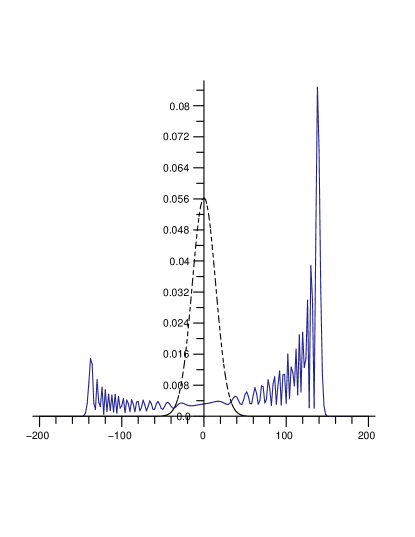
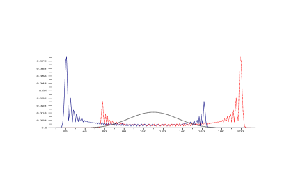
A celebrated result Nayak and Vishwanath (2000); Ambainis et al. (2001) is that this homogeneous quantum walk spreads linearly in time, quadratically faster than classical walks. The shape of the distribution is also very different, as can be seen in Figure 1.
II Inhomogeneous Quantum Walks
Inhomogeneous quantum walks differ from the ones described above in that we allow the coin operator to depend on the position register and the coin register, rather than only on the coin register of the state space. This leads to many interesting new behaviours, such as walks that remain bounded in a certain region for all time, as we shall see.
We will define an inhomogeneous quantum walk in a similar manner to the standard quantum walk, however we now allow the coin operator to be dependent on , the current position of the walk:
| (5) |
In the case of walks on the line could be an arbitrary unitary operator on the two-dimensional coin space. Indeed, there is no need to restrict to walks in which one only moves to the nearest neighbours: more generally, one could allow there to be transitions from a given point to any other point on the line. However for the purposes of most of our discussion of walks on the line we will focus on the simplest case of a transitions to nearest neighbours.
As a first step in this process we will consider a family of examples in which the coin operator is periodic, with the coin operator whose matrix in the basis given by:
| (6) |
Here is an arbitrary positive integer; the period of this walk is . More explicitly, this means that this coin operator transforms states in the following way:
| (7) | ||||
| (8) |
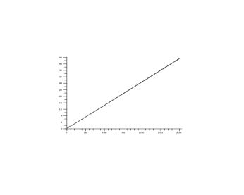
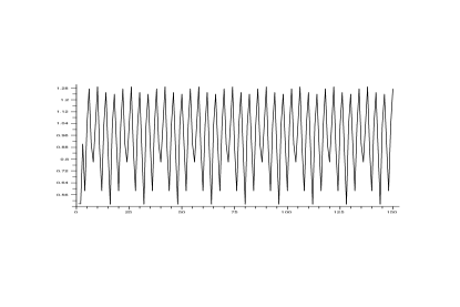
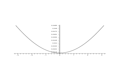
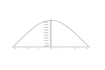
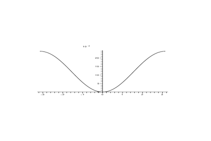
Plots of the standard deviation against the number of time steps for the coin in equation (6) can be seen in figures 2, 3 and 4. They provide some insight into the behaviour that we might expect from these walks, figures 2 and 4 appear to be moving linearly in time and figure 3 appears to be periodic in time. In this section we analyze these cases in detail.
Firstly we consider the general conditions for a walk to be restricted to a finite region of the line for all time:
Lemma 2.1
Let the initial state of the walk to be of the form
| (9) |
then an inhomogeneous quantum random walk with a unitary coin is bounded iff there exists to the left and the right of a coin with matrix of the form
| (10) |
Proof: First assume that the walk is bounded. Then there exists a least upper bound and a greatest lower bound for the walk. Let denote the position of the greatest lower bound and denote the position of the least upper bound. Since is the greatest lower bound for the walk, the walk must reach this point and there is zero probability of moving further left. Hence the coin at must be of the form:
| (11) |
Since the coin is unitary, it must mean that the bottom right component is zero as well. Thus the matrix must be of the following form on the lower bound:
| (12) |
Analogously, since is the least upper bound for the walk, it must mean that at this point there is zero probability of moving to the right. It follows that the coin at must be of the form:
| (13) |
Using the same argument as for the lower bound, the fact that the coin is unitary means that the coin at the upper bound must have the following form:
| (14) |
Therefore, if a random walk is bounded, it must have coins of the above form both above and below the initial state.
Conversely, we now assume that there exists a coin with a matrix of the form (12) both to the left and the right of the initial state. Firstly consider the coin with form (12) to the right of the initial state. The first time the walk approaches this position on the line, it must come from the left. However, the coin above makes everything that is travelling to the right change direction and travel to the left. Thus if amplitude approaches from the left, it will never continue on to the right past that point. Hence this must be an upper bound for the walk.
Similarly, if we consider the coin with the above form to the left of the initial state, it must first be approached from the right. Since the form of the above matrix flips the direction of movement, everything approaching from the right will be reflected. This means that this position on the line must be a lower bound for the walk. Hence, the quantum walk is bounded.
Note that a general initial state is a superposition of states of the type (9); then the condition for boundedness applies separately to each term in the superposition (so, in general, one could have parts of the wave-function that remain bounded in a region and other parts that escape).
As an example, applying this lemma to the coin we defined in equation (6), we can see that the walk will be bounded for even and unbounded for odd .
Now that we understand when a walk will be bounded, we can move on to explore the behaviour when it is unbounded. We would like to calculate the standard deviation of a general periodic walk in order to work out how fast it spreads. We are particularly interested in the family of walks with coin matrix (6). These have even period for any integer . Initially we set up the problem for general walks with even period . Thus we define a general periodic unitary coin with period as follows:
| (15) |
Where and for all . Henceforth we shall omit the in the labelling of , and in order to keep the notation tidy, i.e .
II.1 The Period 6 Case
In order to illustrate the method clearly, we will first use the technique for the case where the period is , i.e. where . We will then move on to define the general case in section II.2.
Starting with the definition of the coin in equation (15) with , one can derive a recurrence relation for the wave function:
| (16) |
Where:
| (21) | ||||
| (24) |
Here is the amplitude of the wave function travelling left at position and time , and is the corresponding amplitude travelling right. i.e.
| (25) |
Recursively substituting the recurrence equation into itself six times, starting from , and yields equations of the form:
| (26) |
where the are constant (i.e. independent of ) matrices given by sums of products of and . There is a simple way of computing these coefficients by referring to Figure 5 . For example

| (27) | |||||
We will change notation at this point to make the equations more concise. We define and grouping certain terms in the sum allows us to write the previous equation as follows:
| (28) |
| (29) |
| (30) |
Discrete Fourier transforming these equations yields the following:
| (31) |
| (32) |
| (33) |
where
| (34) |
Thus we can give an expression for in Fourier space where :
| (35) |
Where the matrix is:
| (36) |
The matrix in equation (35), is unitary, which allows us to write it as:
| (37) |
where is a unitary matrix composed of the eigenvectors of and is a diagonal matrix containing the eigenvalues of . This allows us to rewrite in the following way:
| (38) |
Since the eigenvalues of a unitary matrix lie on the unit circle on the complex plane,
| (39) |
where is the Kronecker delta.
This yields integral expressions for the wave function at arbitrary time and position:
| (40) |
| (41) |
| (42) |
| (43) |
| (44) |
| (45) |
where:
| (46) |
and
| (47) |
We now use the integral expressions in equations (40) to (45) to calculate the first and second moments of the probability distribution on the line. From these we can calculate the standard deviation and thus the rate at which the walk spreads. It is important to note here that we compute these moments only for a number of time steps that is a multiple of six.
The probability that the walk is at position after time steps is given by:
| (48) |
Hence we can calculate the first moment after time steps:
| (49) |
Or more explicity,
| (50) |
Where is the truncated integer part of .
We are interested in the leading order of equation (50) in as because we are calculating the long time variance of the system. We can simplify this expression by noting that the integrals with coefficient in equation (50) are of order using the method of stationary phase.
As we will show that is not the leading order in , we can discard it from our calculation. We can further simplify the expression using:
| (51) |
This yields a much simpler equation for the dominant terms in the expectation of :
| (52) |
For , the exponentials disappear and we are left with terms linear in or constant after the integral over has been performed. Hence these terms give a leading order term assuming that does not vanish. When we can apply the method of stationary phase as , to each term, assuming that the original (35) is non-degenerate (as we will find in the example of particular interest to us - see below) and find that each term is, at most, . Hence we can say that the expectation of has leading order
| (53) |
as .
The second moment for an even number of time steps can be calculated in a similar way using:
| (54) |
However, the and coefficients of are at most and respectively. Since we will show that neither of these are leading order in we can ignore them from the calculation and end up with an expression for the leading order behaviour for the second moment:
| (55) |
Using the same reasoning as before, when we have terms like where , and are constants. Using the method of stationary phase for the other terms yields terms of order less than or equal to . Hence, assuming does not vanish and the leading order term in behaves like as .
Collecting the leading order terms together we find that the leading order term in the variance is
| (56) |
where
| (57) |
The expression (56) is valid for any coin of period six. And given its form - an integral of a sum of terms, each of which is a product of two positive terms - one can see why one might expect, typically, that the leading order behaviour of the standard deviation will indeed to be linear in . We have not been able to get closed form analytic expressions for or (they involve diagonalising a matrix). However in the case that the coin has the matrix with the simple form (with period 6)
| (58) |
and where the initial state is
| (59) |
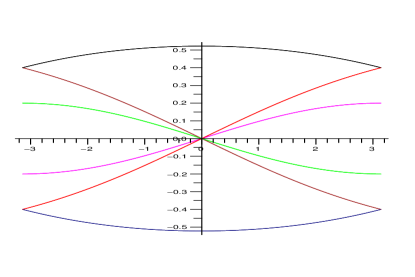
we give figures below plotting and for . These show that the variance does indeed have leading order behaviour proportional to , and hence the spread of the walk is proportional to , as observed in the earlier figure 2.
II.2 The General Case
Very similar calculations can be performed for the period case, for general , leading to an expression for the leading order behaviour exactly analogous to that for the period six case:
| (60) |
where
| (61) |
The functions and arise, as in the period six case, from the initial condition and diagonalization of the unitary matrix defining the time evolution:
| (62) |
III Quantum Walks Defined Via Double-Reflection
In Szegedy (2004), Szegedy proposed a method for defining the quantum walk on a graph starting with a classical Markov chain. The work was generalized in Magniez et al. (2007b). For reasons that will be clear shortly, we refer to these quantum walks as “double-reflection” walks.
We now compare the construction we have been using with that in Szegedy (2004); Magniez et al. (2007b) for the particular case of motion on the line. The state space used in Szegedy (2004); Magniez et al. (2007b) consists of two copies of the position space, rather than a position and coin register. Thus the Hilbert space is spanned by . We can describe the coin based walks using this Hilbert space by identifying with and with .
In the case of motion on a line, a double-reflection walk is set up as follows Szegedy (2004); Magniez et al. (2007b). Let and be complex numbers satisfying
| (63) |
The two-step walk operator is defined via the following equations:
| (64) |
| (65) |
| (66) |
The Hadamard walk in the double-reflection framework can be realized by setting:
| (67) |
The inhomogeneous quantum walk with coin in equation (6) can be reproduced by taking:
| (68) |
Although the original walks in Szegedy (2004) have real amplitudes, it is natural to allow the constants and be complex numbers as in Magniez et al. (2007b). We now show that even if we allow this, not all walks produced by the position-dependant coin construction can be realized by walks of the form (66).
Using a generalized double-reflection form of the quantum walk to yields:
| (69) |
We now wish to compare this to a walk using a controlled unitary coin. Since we have allowed the “forward” and “backward” steps to be different in (LABEL:W-S-psi-0), we need to take this into account. So for two steps of the position-dependent-coin walk we use different coin operators in the first and second step.
We consider a two general controlled unitary coins, described in the Hilbert space of two copies of the position register:
| (70) |
and
| (71) |
The general two-step walk operator associated with these coins is given by:
| (72) |
where
| (73) |
| (74) |
and
| (75) |
Let with . Applying walk operator yields:
| (76) |
We can now see that the effect of can be reproduced by a walk using a position-dependent coins by choosing , , and , , .
However the most general walk of the form (LABEL:W-S-psi-0) cannot reproduce all walks with position dependent coins. This is because from (LABEL:W-S-psi-0) one can see that
| (77) |
is real for any choice of and , however
| (78) |
which need not be real. Indeed even if we take both steps of the position-dependent-coin walk to be the same (as is usually done), we get
| (79) |
and still the most general walk of the form (LABEL:W-S-psi-0) cannot reproduce all walks with position dependent coins.
Indeed it is not too difficult to check that even if one allows transitions to arbitrary positions in the double-reflection form of the walk, it cannot reproduce all walks defined by position-dependent coins. For let us take general states of the form
| (80) |
rather than (64). The matrix element
| (81) |
is still real.
We also note that for some purposes it is natural to use the shift operator
| (82) |
rather than (2). This is a closer analogue of the shift embodied in the double-reflection framework. It is straightforward to check, however, that this does not alter our conclusions: this modified version of the position-dependent-coin walk can also reproduce the double-reflection walk; and not all position-dependent-coin walks with this modified shift can be realized by double-reflection walks.
Nonetheless, there may be a generalization of the double-reflection form of the quantum walk which allows for these two constructions to be equivalent; this question is left open for future work.
IV The Pólya Urn
The classical Pólya Urn is a model in which there is an urn containing a number of red and black balls. At every time step one is drawn at random, then replaced with a copy of the drawn ball. Let be a random variable representing the number of red balls in an urn containing balls in total. Let the random variable be given by , then it is possible to show that almost surely as , where and are the initial number of red and black balls in the urn respectively, and is a beta distribution with parameters and . Freedman (1965).
The classical system is not irreducible so it does not fit naturally into the double-reflection framework. It is nonetheless instructive to see what happens if we try to use that framework to quantize this system.
A natural position space is spanned by where and are the numbers of red and black balls respectively. In the classical model a time step increases the number of red or black balls by one so it is natural to try to set up a quantum model by taking something like the following:
| (83) |
| (84) |
| (85) |
where are constants.
However it may easily be checked that this system has the following behaviour
-
•
for each pair the two-dimensional subspace spanned by and is invariant under the time evolution (so if the starting state of our walk is in this subspace, it just moves around in the subspace)
-
•
similarly for each pair the two-dimensional subspace spanned by and is invariant under the time evolution
-
•
all other states are unchanged by the time evolution
In particular the number of red or black balls does not increase with time by more than one from its initial value. Thus this quantum evolution does not seem to be the natural quantum version of the classical model. It would be interesting to know whether it is possible to use different states than (83) to produce a double-reflection quantization of the Pólya Urn that is more satisfactory (i.e. one that only increases the number of red and black balls as time evolves), but we have not yet been able to do so.
It turns out to be relatively straightforward to set up a quantum walk with a position-dependent coin that seems to capture how a quantum version of the Pólya Urn should behave, as we now describe.
The state space is spanned by and . The first two registers are the number of red and black balls and the third register can be in one of two states or corresponding to whether the number of red or black balls is to increase in the “shift” step of the walk. We are really only interested in the number of red and black balls and being positive, but in order for the walk to be unitary it will be convenient to allow and to take any integer values (although we will typically only be interested in initial states with and ). So we set up our walk as follows. The coin operator is defined by:
| (86) |
| (87) |
| (88) |
| (89) |
An attractive feature of this walk is that if you run one step of the walk, measure the system and reset the chirality state to , then the classical walk is recovered.
The resulting probability distribution of running this walk, starting with 10 red balls and 10 black balls for 200 time steps, can be seen in Figure 10.
There is a heavy bias to the right, similar to the Hadamard random walk. It is possible to reduce the bias using a more symmetric coin and initial condition.
The quantum Pólya urn plot shows several features that one might expect, such as most of the probability being concentrated to the far right or left. This is to be expected, as the Pólya urn is an example of a reinforced process; if an event occurs then it becomes more likely to occur in the future.
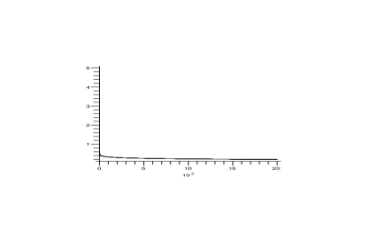
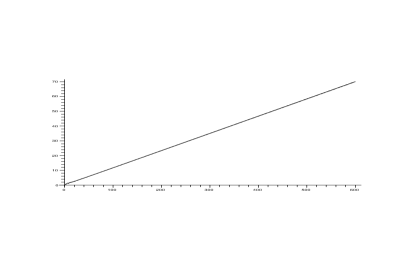
We also calculated the standard deviation of the Pólya Urn quantum walk numerically, and a plot of this divided by the number of timesteps can be seen in Figure 11. For the walk to evolve linearly in time asymptotically as , one would expect this graph to tend towards a horizontal line. This appears to be the case, but a proof of asymptotic linear evolution is an open question for future work as the quantum Pólya Urn has a non-periodic coin and thus our original method for periodic coins can not be applied.
V Conclusions
In this paper we have analyzed some particular models of inhomogeneous walks. It would be interesting to understand whether one can make general characterizations of the long-time behaviour of quantum walks from knowledge of their (position-dependent) coins. For example we have described walks that are bounded and others whose spread is linear in time. We do not know what intermediate types of behaviour are possible. It would also be interesting to know whether quantum walks (including non-periodic ones) “typically” spread linearly in time. It would also be attractive to understand the relationship between the double-reflection and position-dependent-coin walks more fully: is there a suitable generalization that encompasses both?
Acknowledgements.
We are very grateful to Aram Harrow, Miklos Santha and Andreas Winter for many insightful observations. We also gratefully acknowledge support for this work from: the UK EPSRC through the QIP-IRC, the University of Bristol for a Research Fellowship and the EU through the project QAP.References
- Aharonov et al. (1993) Y. Aharonov, L. Davidovich, and N. Zagury, Phys. Rev. A 48, 1687 (1993).
- Meyer (1996a) D. Meyer, J. Stat. Phys. 85, 551 (1996a).
- Meyer (1996b) D. Meyer, Phys. Lett. A 223, 337 (1996b).
- Watrous (2001) J. Watrous, Journal of Computer and System Sciences 62, 376 (2001).
- Shenvi et al. (2003) N. Shenvi, J.Kempe, and K. Whaley, Physical Review A 67 (2003).
- Ambainis (2007) A. Ambainis, SIAM Journal on Computing 37, 210 (2007).
- Buhrman and Spalek (2006) H. Buhrman and R. Spalek, Proc. 17th ACM-SIAM Symposium on Discrete Algorithms p. 880 (2006).
- Magniez and Nayak (2007) F. Magniez and A. Nayak, Algorithmica 48, 221 (2007).
- Magniez et al. (2007a) F. Magniez, M. Santha, and M. Szegedy, SIAM Journal of Computing 37, 413 (2007a).
- Ambainis (2003) A. Ambainis, International Journal of Quantum Information 1, 507 (2003).
- Ambainis et al. (2005) A. Ambainis, J. Kempe, and A. Rivosh, Proc. 16th ACM-SIAM SODA p. 1099 (2005).
- Santha (2008) M. Santha, 5th Theory and Applications of Models of Computation (TAMC08), Xian, April 2008, LNCS 4978 p. 31 (2008).
- Szegedy (2004) M. Szegedy, in FOCS ’04: Proceedings of the 45th Annual IEEE Symposium on Foundations of Computer Science (IEEE Computer Society, Washington, DC, USA, 2004), pp. 32–41, ISBN 0-7695-2228-9.
- Magniez et al. (2007b) F. Magniez, A. Nayak, J. Roland, and M. Santha, Proc. 39th ACM Symposium on the Theory of Computing p. 575 (2007b).
- Nayak and Vishwanath (2000) A. Nayak and A. Vishwanath, arXiv:quant-ph/0010117 (2000).
- Ambainis et al. (2001) A. Ambainis, E. Bach, A. Nayak, A. Vishwanath, and J. Watrous, Proceedings of the 33rd Annual AMC Symposium on Theory of Computing pp. 37–49 (2001).
- Freedman (1965) D. A. Freedman, Ann. Math. Statist. 36, 956 (1965).