Stochastic Background of Relic Scalar Gravitational Waves tuned by Extended Gravity

Abstract

A stochastic background of relic gravitational waves is achieved by the so called adiabatically-amplified zero-point fluctuations process derived from early inflation. It provides a distinctive spectrum of relic gravitational waves. In the framework of scalar-tensor gravity, we discuss the scalar modes of gravitational waves and the primordial production of this scalar component which is generated beside tensorial one. Then we analyze different viable $f(R)$-gravities towards the Solar System tests and stochastic gravitational waves background. The aim is to achive experimental bounds for the theory at local and cosmological scales in order to select models capable of addressing the accelerating cosmological expansion without cosmological constant but evading the weak field constraints. It is demonstrated that viable $f(R)$-gravities under consideration not only satisfy the local tests, but additionally, pass the PPN-and stochastic gravitational waves bounds for large classes of parameters.

1 Introduction

The idea that General Relativity (GR) should be extended or corrected at large scales (infrared limit) or at high energies (ultraviolet limit) is suggested by several theoretical and observational issues [1]. Quantum field theory in curved spacetimes, as well as the low-energy limit of String/M theory, both imply semi-classical effective actions containing higher-order curvature invariants or scalar-tensor terms. In addition, GR has been definitely tested only at Solar System scales while it may show several shortcomings if checked at higher energies or larger scales. Besides, the Solar System experiments are, up to now, not conclusive to state that the only viable theory of gravity is GR: for example, the limits on PPN parameters should be greatly improved to fully remove degeneracies. Of course, modifying the gravitational action asks for several fundamental challenges. These models can exhibit instabilities or ghost - like behavior, while, on the other hand, they have to be matched with observations and experiments in the appropriate low energy limit. there exist cosmological solutions that give the accelerated expansion of the universe at late times. In addition, it has been discovered that some stability conditions can lead to avoid ghost and tachyon solutions. Furthermore there exist viable $f(R)$ models which satisfy both background cosmological constraints and stability conditions and results have been achieved in order to place constraints on $f(R)$ cosmological models by CMBR anisotropies and galaxy power spectrum. Moreover, some of such viable models lead to the unification of early-time inflation with late-time acceleration. On the other hand, by considering $f(R)$-gravity in the low energy limit, it is possible to obtain corrected gravitational potentials capable of explaining the flat rotation curves of spiral galaxies or the dynamics of galaxy clusters without considering huge amounts of dark matter. Furthermore, several authors have dealt with the weak field limit of fourth order gravity, in particular considering the PPN limit and the spherically symmetric solutions. This great deal of work needs an essential issue to be pursued: we need to compare experiments and probes at local scales (e.g. Solar System) with experiments and probes at large scales (Galaxy, extragalactic scales, cosmology) in order to achieve self-consistent $f(R)$ models. In order to constrain further viable $f(R)$-models, one could take into account also the stochastic background of gravitational waves (GW) which, together with cosmic microwave background radiation (CMBR), would carry a huge amount of information on the early stages of the Universe evolution. In fact, if detected, such a background could constitute a further probe for these theories at very high red-shift [9]. On the other hand, a key role for the production and the detection of the relic gravitational radiation background is played by the adopted theory of gravity . This means that the effective theory of gravity should be probed at zero, intermediate and high redshifts to be consistent at all scales and not simply extrapolated up to the last scattering surface, as in the case of GR.

The aim of this report is to discuss the PPN Solar-System constraints and the GW stochastic background considering some recently proposed $f(R)$ gravity models [2, 3] which satisfy both cosmological and stability conditions mentioned above. Using the definition of PPN-parameters $\gamma$ and $\beta$ in terms of $f(R)$-models and the definition of scalar GWs [4], we compare and discuss if it is possible to search for parameter ranges of $f(R)$-models working at Solar System and GW stochastic background scale [5].

2 Extended Gravity

A action for scalar-tensor gravity in a Brans-Dicke-like form which can be adopted also for $f(R)$-gravity once a suitable scalar field is defined, is [6]

$$S=\int d^{4}x\sqrt{-g}\left[\varphi R-\frac{\omega(\varphi)}{\varphi}g^{\mu\nu}\varphi_{;\mu}\varphi_{;\nu}-W(\varphi)+\mathcal{L}_{m}\right]$$ (1)

By varying the action (1) with respect to $g_{\mu\nu}$, we obtain the field equations

$$\begin{array}[]{c}G_{\mu\nu}=-\frac{4\pi\tilde{G}}{\varphi}T_{\mu\nu}^{(m)}+\frac{\omega(\varphi)}{\varphi^{2}}(\varphi_{;\mu}\varphi_{;\nu}-\frac{1}{2}g_{\mu\nu}g^{\alpha\beta}\varphi_{;\alpha}\varphi_{;\beta})\\ \\ +\frac{1}{\varphi}(\varphi_{;\mu\nu}-g_{\mu\nu}\square\varphi)+\frac{1}{2\varphi}g_{\mu\nu}W(\varphi)\end{array}$$ (2)

while the variation with respect to $\varphi$ gives the Klein - Gordon equation

$$\square\varphi=\frac{1}{2\omega(\varphi)+3}[-4\pi\tilde{G}T^{(m)}$$

$$+2W(\varphi)+\varphi W^{\prime}(\varphi)+\frac{d\omega(\varphi)}{d\varphi}g^{\mu\nu}\varphi_{;\mu}\varphi_{;\nu}].$$

(3)

We are assuming physical units $G=1$, $c=1$ and $\hbar=1$. $T_{\mu\nu}^{(m)}$ is the matter stress-energy tensor and $\tilde{G}$ is a dimensional, strictly positive, gravitational coupling constant [4, 7]. The Newton constant is replaced by the effective coupling

$$G_{eff}=-\frac{1}{2\varphi},$$ (4)

which is, in general, different from $G$. GR is recovered for

$$\varphi=\varphi_{0}=-\frac{1}{2}.$$ (5)

3 Gravitational waves from Extended Gravity

In order to study gravitational waves, we assume first-order, small perturbations in vacuum ($T_{\mu\nu}^{(m)}=0$). This means

$$g_{\mu\nu}=\eta_{\mu\nu}+h_{\mu\nu}\,,\qquad\varphi=\varphi_{0}+\delta\varphi$$ (6)

and

$$W\simeq\frac{1}{2}\alpha\delta\varphi^{2}\Rightarrow W^{\prime}\simeq\alpha\delta\varphi$$ (7)

for the self-interacting, scalar-field potential. These assumptions allow to derive the "linearized" curvature invariants $\widetilde{R}_{\mu\nu\rho\sigma}$ , $\widetilde{R}_{\mu\nu}$ and $\widetilde{R}$ which correspond to $R_{\mu\nu\rho\sigma}$ , $R_{\mu\nu}$ and $R$, and then the linearized field equations [4, 8]

$$\begin{array}[]{c}\widetilde{R}_{\mu\nu}-\frac{\widetilde{R}}{2}\eta_{\mu\nu}=-\partial_{\mu}\partial_{\nu}\Phi+\eta_{\mu\nu}\square\Phi\\ \\ {}\square\Phi=m^{2}\Phi,\end{array}$$ (8)

where

$$\Phi\equiv-\frac{\delta\varphi}{\varphi_{0}}\,,\qquad m^{2}\equiv\frac{\alpha\varphi_{0}}{2\omega+3}\,.$$ (9)

In particular, the transverse-traceless (TT) gauge (see [8]) can be generalized to scalar-tensor gravity obtaining the total perturbation of a GW incoming in the $z+$ direction in this gauge as

$$h_{\mu\nu}(t-z)=A^{+}(t-z)e_{\mu\nu}^{(+)}+A^{\times}(t-z)e_{\mu\nu}^{(\times)}$$

$$+\Phi(t-z)e_{\mu\nu}^{(s)}.$$ (10)

The term $A^{+}(t-z)e_{\mu\nu}^{(+)}+A^{\times}(t-z)e_{\mu\nu}^{(\times)}$ describes the two standard (i.e. tensorial) polarizations of a gravitational wave arising from GR in the TT gauge [8], while the term $\Phi(t-z)e_{\mu\nu}^{(s)}$ is the extension of the TT gauge to the scalar case. This means that, in scalar-tensor gravity, the scalar field generates a third component for the tensor polarization of GWs. This is because three different degrees of freedom are present of [4, 10], while only two are present in standard General Relativity.

4 Stochastic background of relic scalar GWs

Then, for a purely scalar gravitational wave, the metric perturbation is [4, 10, 9]

$$h_{\mu\nu}=\Phi\,e_{\mu\nu}^{(s)}\;.$$ (11)

The stochastic background of scalar gravitational waves can be described in terms of the scalar field $\Phi$ and characterized by a dimensionless spectrum (see the analogous definition for tensor modes in [4])

$$\Omega_{sgw}(f)=\frac{1}{\rho_{c}}\frac{d\rho_{sgw}}{d\ln f}\;,$$ (12)

where

$$\rho_{c}\equiv\frac{3H_{0}^{2}}{8\pi G}$$ (13)

is the (present) critical energy density of the universe, $H_{0}$ is the Hubble parameter today, and $d\rho_{sgw}$ is the energy density of the scalar gravitational radiation in the frequency interval $\left(f,f+df\right)$. We are now using standard units. Now it is possible to write an expression for the energy density of the stochastic scalar relic gravitons background in the angular frequency interval $(\omega,\omega+d\omega)$ as

$$d\rho_{sgw}=2\hbar\omega\left(\frac{\omega^{2}d\omega}{2\pi^{2}c^{3}}\right)N_{\omega}=$$

$$\frac{\hbar H_{dS}^{2}H_{0}^{2}}{4\pi^{2}c^{3}}\frac{d\omega}{\omega}=\frac{\hbar H_{dS}^{2}H_{0}^{2}}{4\pi^{2}c^{3}}\frac{df}{f}\,,$$ (14)

where $f$, as above, is the frequency in standard comoving time. Eq. (14) can be rewritten in terms of the critical and de Sitter energy densities

$$H_{0}^{2}=\frac{8\pi G\rho_{c}}{3c^{2}}\,,\qquad H_{dS}=\frac{8\pi G\rho_{dS}}{3c^{2}}\;.$$ (15)

Introducing the Planck density ${\displaystyle\rho_{Planck}=\frac{c^{5}}{\hbar G^{2}}}$, the spectrum is given by

$$\Omega_{sgw}(f)=\frac{1}{\rho_{c}}\frac{d\rho_{sgw}}{d\ln f}=\frac{f}{\rho_{c}}\frac{d\rho_{sgw}}{df}=\frac{16}{9}\frac{\rho_{dS}}{\rho_{Planck}}\;.$$ (16)

At this point, some comments are in order. First, the calculation works for a simplified model that does not include the matter-dominated era. If the latter is included, the redshift at the equivalence epoch has to be considered. Taking into account Ref. [4, 10] one gets

$$\Omega_{sgw}(f)=\frac{16}{9}\frac{\rho_{dS}}{\rho_{Planck}}(1+z_{eq})^{-1}$$ (17)

for the waves which, at the epoch in which the universe becomes matter-dominated, have a frequency higher than $H_{eq}$, the Hubble parameter at equivalence. This situation corresponds to frequencies $f>(1+z_{eq})^{1/2}H_{0}$ today. The redshift correction in eq. (17) is needed since the present value of the Hubble parameter $H_{0}$ would be different without a matter-dominated contribution. At lower frequencies, the spectrum is given by

$$\Omega_{sgw}(f)\propto f^{-2}.$$ (18)

Nevertheless, since the spectrum falls off as $f^{-2}$ at low frequencies, today at LIGO/VIRGO and LISA frequencies, one gets

$$\Omega_{sgw}(f)h_{100}^{2}<2.3\times 10^{-12}\;,$$ (19)

where $h_{100}=H_{0}/\left(100\;\mbox{km}\cdot\mbox{s}^{-1}\cdot\mbox{Mpc}^{-1}\right)$. It is interesting to calculate the corresponding strain at $f\sim 100$Hz, where interferometers such as VIRGO and LIGO achieve maximum sensitivity. The well known equation for the characteristic amplitude adapted to the scalar component of gravitational waves

$$\Phi_{c}(f)\simeq 1.26\times 10^{-18}\left(\frac{1\,\mbox{Hz}}{f}\right)\sqrt{h_{100}^{2}\Omega_{sgw}(f)}\;,$$ (20)

can be used to obtain

$$\Phi_{c}\left(100\,\mbox{Hz}\right)<2\cdot 10^{-26}\;.$$ (21)

Then, since we expect a sensitivity of the order of $10^{-22}$ for the above interferometers at $f\sim 100$ Hz, we need to gain four orders of magnitude. Let us analyze the situation also at lower frequencies. The sensitivity of the VIRGO interferometer is of the order of $10^{-21}$ at $f\sim 10$ Hz and in that case it is

$$\Phi_{c}\left(10\,\mbox{Hz}\right)<2\cdot 10^{-25}\;.$$ (22)

The sensitivity of the LISA interferometer will be of the order of $10^{-22}$ at $f\sim 10^{-3}$ Hz and in this case it is

$$\Phi_{c}\left(10^{-3}\mbox{Hz}\right)<2\cdot 10^{-21}\;.$$ (23)

This means that a stochastic background of relic scalar gravitational waves could, in principle, be detected by the LISA interferometer [11].

5 $f(R)$-gravity constrained by PPN parameters and stochastic background of GWs

A Brans-Dike-like theory with $\omega=0$ is dinamically equivalent to an $f(R)$-gravity, so the bounds coming from the interferometric ground-based (VIRGO, LIGO) and space (LISA) experiments could constitute a further probe for gravity if matched with bounds at other scales to achieve experimental bounds for the theory at local and cosmological scales . For our aims consider a class of $f(R)$ models which do not contain cosmological constant and are explicitly designed to satisfy cosmological and Solar-System constraints in given limits of the parameter space. In practice, we choose a class of functional forms of $f(R)$ capable of matching, in principle, observational data. Firstly, the cosmological model should reproduce the CMBR constraints in the high-redshift regime (which agree with the presence of an effective cosmological constant). Secondly, it should give rise to an accelerated expansion, at low redshift, according to the $\Lambda$CDM model. Thirdly, there should be sufficient degrees of freedom in the parameterization to encompass low redshift phenomena (e.g. the large scale structure) according to the observations. Finally, small deviations from GR should be consistent with Solar System tests. All these requirements suggest that we can assume the limits

$$\lim_{R\rightarrow\infty}f(R)={\rm constant},$$ (24)

$$\lim_{R\rightarrow 0}f(R)=0,$$ (25)

which are satisfied by a general class of broken power law models, proposed in [3], which are

$$f_{HS}(R)=R-\lambda R_{c}\frac{\left(\frac{R}{R_{c}}\right)^{2n}}{\left(\frac{R}{R_{c}}\right)^{2n}+1}$$ (26)

where $m$ is a mass scale and $c_{1,2}$ are dimensionless parameters. Besides, another viable class of models was proposed in [2]

$$f_{S}(R)=R+\lambda R_{c}\left[\left(1+\frac{R^{2}}{R_{c}^{2}}\right)^{-p}-1\right]\,.$$ (27)

Since $f(R=0)=0$, the cosmological constant has to disappear in a flat spacetime. The parameters $\{n$, $p$, $\lambda$, $R_{c}\}$ are constants which should be determined by experimental bounds. In Fig.(1), we have plotted the selected models as function of ${\displaystyle\frac{R}{R_{c}}}$ for suitable values of $\{p,n,\lambda\}$ .

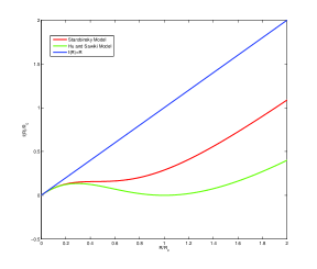
Figure 1: Plots of $f(R)$ models as function of $\frac{R}{R_{c}}$. Model $f_{HS}$ in Eq. (26) with $n=1$ and $\lambda=2$ (green line). Model $f_{S}$ in Eq.(27) with $p=2$, $\lambda=0.95$ (red line). We also plot $f(R)=R$ (blu line) to see whether or not the stability condition $f_{,R}>0$ is violated.

The above models can be constrained at Solar System level by considering the PPN formalism. This approach is extremely important in order to test gravitational theories and to compare them with GR. One can derive the PPN-parameters $\gamma$ and $\beta$ in terms of a generic analytic function $f(R)$ and its derivative

$$\gamma-1=-\frac{f^{\prime\prime}(R)^{2}}{f^{\prime}(R)+2f^{\prime\prime}(R)^{2}}\,,$$ (28)

$$\beta-1=\frac{1}{4}\left[\frac{f^{\prime}(R)\cdot f^{\prime\prime}(R)}{2f^{\prime}(R)+3f^{\prime\prime}(R)^{2}}\right]\frac{d\gamma}{dR}\,.$$ (29)

These quantities have to fulfill the constraints coming from the Solar System experimental tests. They are the perihelion shift of Mercury , the Lunar Laser Ranging , the upper limits coming from the Very Long Baseline Interferometry (VLBI) and the results obtained from the Cassini spacecraft mission in the delay of the radio waves transmission near the Solar conjunction.

• Mercury perihelion Shift $\left|2\gamma-\beta-1\right|<3\times 10^{-3}$

• Lunar Laser Ranging $4\beta-\gamma-3=(0.7\pm 1)\times 10^{-3}$

• Very Long Baseline Interferometer $\left|\gamma-1\right|<4\times 10^{-4}$

• Cassini Spacecraft $\gamma-1=(2.1\pm 2.3)\times 10^{-5}$

Take into account the above $f(R)$-models,specifically, we have investigated the values or the ranges of parameters in which they match the above Solar-System experimental constraints. In other words, we use these models to search under what circumstances it is possible to significantly address cosmological observations by $f(R)$-gravity and, simultaneously, evade the local tests of gravity [5]. At this point, using the above LIGO, VIRGO and LISA upper bounds, calculated for the characteristic amplitude of GW scalar component, let us test the $f(R)$-gravity models. Taking into account the discussion in Sec. 2, we have that the GW scalar component is derived considering

$$\Phi=-\frac{\delta\sigma}{\sigma_{0}}\,,\qquad\sigma=-\ln(1+f^{\prime}(R))=\ln f^{\prime}(A)\,,$$

$$\qquad\delta\sigma=\frac{f^{\prime\prime}(A)}{1+f^{\prime}(A)}\delta A\,.$$ (30)

Finally we obtain a good sets of parameters for the Starobinsky model PPN vs GW-stochastic:

• $\frac{R}{R_{c}}=3.38$  , $p=1$  , $\lambda=2$

• $\frac{R}{R_{c}}=\sqrt{3}$  , $p=2$  , $0.944<\lambda<0.966$

and for Hu and Sawiki model

• $\frac{R}{R_{c}}=\sqrt{3}$  , $n=2$  , $\lambda>\frac{8}{3\sqrt{3}}$

such sets of parameters are not in conflict with bounds coming from the cosmological stochastic background of GWs and, some sets reproduce quite well both the PPN upper limits and the constraints on the scalar component amplitude of GWs. The results indicate that self-consistent models could be achieved comparing experimental data at very different scales without extrapolating results obtained only at a given scale [5].

6 Conclusions

We have investigated the possibility that some viable $f(R)$ models could be constrained considering both Solar System experiments and upper bounds on the stochastic background of gravitational radiation. Such bounds come from interferometric ground-based (VIRGO and LIGO) and space (LISA) experiments. The underlying philosophy is to show that the $f(R)$ approach, in order to describe consistently the observed universe, should be tested at very different scales, that is at very different redshifts. In other words, such a proposal could partially contribute to remove the unpleasant degeneracy affecting the wide class of dark energy models, today on the ground.

Beside the request to evade the Solar System tests, new methods have been recently proposed to investigate the evolution and the power spectrum of cosmological perturbations in $f(R)$ models. The investigation of stochastic background, in particular of the scalar component of GWs coming from the $f(R)$ additional degrees of freedom, could acquire, if revealed by the running and forthcoming experiments, a fundamental importance to discriminate among the various gravity theories [9]. These data (today only upper bounds coming from simulations) if combined with Solar System tests, CMBR anisotropies, LSS, etc. could greatly help to achieve a self-consistent cosmology bypassing the shortcomings of $\Lambda$CDM model.

Specifically, we have taken into account two broken power law $f(R)$ models fulfilling the main cosmological requirements which are to match the today observed accelerated expansion and the correct behavior in early epochs. We have taken into account the results of the main Solar System current experiments. Such results give upper limits on the PPN parameters which any self-consistent theory of gravity should satisfy at local scales. Starting from these, we have selected the $f(R)$ parameters fulfilling the tests. As a general remark, all the functional forms chosen for $f(R)$ present sets of parameters capable of matching the two main PPN quantities, that is $\gamma_{exp}$ and $\beta_{exp}$. This means that, in principle, extensions of GR are not a priori excluded as reasonable candidates for gravity theories. To construct such extensions, the reconstruction method developed in may be applied.

The interesting feature, and the main result of this paper, is that such sets of parameters are not in conflict with bounds coming from the cosmological stochastic background of GWs. In particular, some sets of parameters reproduce quite well both the PPN upper limits and the constraints on the scalar component amplitude of GWs [5, 11].

Far to be definitive, these preliminary results indicate that self-consistent models could be achieved comparing experimental data at very different scales without extrapolating results obtained only at a given scale.

References

- [1] S. Capozziello and M. Francaviglia, Gen.Rel.Grav. 40, pp 357-420, (2008).
- [2] A. A. Starobinsky, JETP Lett. 86, 157 (2007).
- [3] W. Hu and I. Sawicki, Phys. Rev. D 76 064004 (2007).
- [4] S.Capozziello, C.Corda, M. De Laurentis, Mod. Phys. Lett. A, vol. 22, 2647,(2007).
- [5] S. Capozziello, M. De Laurentis, S. Nojiri, S.D. Odintsov, e-Print: arXiv:0808.1335 [hep-th].
- [6] C. Brans and R. H. Dicke, Phys. Rev. 124, 925 (1961).
- [7] S. Capozziello, Quantum Gravity Research Trends Ed. A. Reimer, pp. 227-276 Nova Science Publishers Inc., NY (2005).
- [8] C. W. Misner , K. S. Thorne and J. A. Wheeler, “Gravitation” - W. H. Feeman and Company 1973.
- [9] S.Capozziello, C.Corda, M. De Laurentis Mod. Phys. Lett. A vol. 22 ,1097 (2007).
- [10] S.Capozziello, C.Corda, M. De Laurentis, Phys. Lett. B 699, 255-259 (2008).
- [11] S. Bellucci, S. Capozziello, M. De Laurentis, V. Faraoni, Phys. Rev. D 79, 104004 (2009).